1. Introduction and notation¶
[Source: include/PBeFS/astar/Domain.h (the concepts of a
problem), include/PBeFS/astar/Solution.h (Solution,
SearchStats, SearchOptions),
include/PBeFS/astar/Node.h (cost_slack,
infinite_cost), include/PBeFS/core/SearchUtils.h
(ParallelParams,
run_workers, pin_worker), include/PBeFS/astar/HDAStar.h
(ParallelOptions)]
We are concerned with finding a path of least cost from an initial state
to a goal state of a graph that is far too large to be written down, but
whose states and edges can be generated on demand from a few rules (the
moves of a puzzle, the roads of a map, the actions of a plan). This
chapter fixes the problem and the notation shared by the whole book
(§1.1), discusses what makes an instance of the problem hard
(§1.2) and by which measures a search is judged
(§1.3), and lists the conventions of the pseudocode
(§1.4). It then describes how a problem is handed to the
library, i.e., the concept Domain and its refinements, and what a search
returns (§1.5), how the parallel searches are run on threads,
OpenMP, FastFlow or MPI (§1.6), and the plan of the book
(§1.7). Thus, the searches themselves start in
Chapter 2, while the problems used as examples
throughout are described in Chapter 14.
1.1 The state-space problem¶
The model of this book is the deterministic one with perfect information: the agent knows the state of the world, and an action applied to a state leads to one state only, known in advance. Stochastic outcomes (Markov decision processes), partial observations, adversaries (two-player games) and the interleaving of planning with acting (real-time search) are not treated, and for them we refer to the textbook of Russell and Norvig [13]. Our definitions follow Edelkamp and Schrödl [10] (chapter 1) and Russell and Norvig [13] (chapter 3).
Definition 1.1 (State-space problem). A state-space problem is a tuple \(P = (S, A, s_0, T, w)\), where \(S\) is a set of states, \(s_0 \in S\) the initial state, \(T \subseteq S\) the set of goal states, and \(A\) a set of actions. Each action \(a \in A\) is a partial map \(a : S \to S\) (defined on the states where \(a\) is applicable), and \(w\) assigns to the application of \(a\) to \(s\) a cost \(w(s, a) \ge 0\). A solution is a sequence of actions \(\pi = (a_1, \ldots, a_k)\) such that the states \(u_0 = s_0\) and \(u_i = a_i(u_{i-1})\) are defined and \(u_k \in T\); its cost is \(\sum_{i=1}^k w(u_{i-1}, a_i)\). One asks for a solution of least cost. When each action costs 1 the problem is said to have unit costs, and the cost of a solution is then its length.
In fact, the problem is a shortest-path problem: the state-space graph of \(P\) is the directed graph \(G = (V, E)\) with \(V = S\) and an edge \((u, v) \in E\) whenever \(v = a(u)\) for some action \(a\) applicable to \(u\), with the cost \(c(u, v)\) of the cheapest such action. A solution is then a path from \(s_0\) to a node of \(T\), and its cost is the sum of the costs of its edges. Since only the cheapest action between two states matters, we state the problem on the graph from now on, and we use state and node interchangeably whenever no confusion arises (the distinction is made in Chapter 2, where a node is the record that a search keeps for a state). Several actions, or several paths, usually lead to the same state; hence, the graph is not a tree in general, and a search that does not recognize the states it has already met (a duplicate) may do the same work many (possibly exponentially many) times.
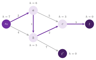
The graph of Figure 1.1 is small enough to be stored as a list of edges, or as an adjacency matrix of \(|V|^2\) entries. However, the graphs of interest are not: the 15-puzzle has \(16!/2 \approx 1.05 \cdot 10^{13}\) states reachable from any of its states (a rather "small" puzzle, see §14.2), whose adjacency matrix would have more than \(10^{26}\) entries, and a map of a video game, a routing problem or a planning task are of the same kind. Such a graph is given implicitly.
Definition 1.2 (Implicit graph). An implicit state-space graph is given by the initial state \(s_0\), a predicate \(\mathrm{goal} : V \to \{\mathrm{false}, \mathrm{true}\}\) that recognizes the goals, and an expansion procedure that, given a state \(u\), enumerates the successors \(v\) of \(u\), i.e., the states with \((u, v) \in E\), each with the cost \(c(u, v)\) of its edge. A state is generated when it is first produced by an expansion (or when it is \(s_0\)), and expanded when its own successors are enumerated.
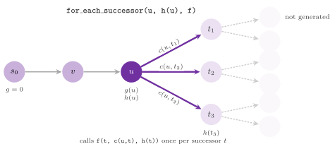
Hence, the searches of this book only see the graph through these three objects, and the part of the graph that they hold in memory is the part they have generated; the rest of \(V\) is never built (Figure 1.2). We assume throughout that the graph is locally finite, i.e., that each state has finitely many successors (while \(V\) may be infinite), and that the costs are nonnegative, \(c(u, v) \ge 0\). Edges of cost 0 are allowed (e.g., the moves of the player of Sokoban that push no box). Negative costs are not, since with them the optimal cost may not exist and the searches that expand the states by a nondecreasing priority are not correct.
The cost functions¶
We denote by \(g^*(u)\) the least cost of a path from \(s_0\) to \(u\), by \(h^*(u)\) the least cost of a path from \(u\) to a goal (\(+\infty\) if no goal is reachable from \(u\)), and by \(C^* = h^*(s_0)\) the optimal cost, which is the value sought (in Figure 1.1, \(C^* = 8\)). A search keeps, for each state \(u\) it has generated, the cost \(g(u)\) of the best path from \(s_0\) to \(u\) found so far; this is the cost of an actual path, and hence \(g(u) \ge g^*(u)\) at any time. It also keeps the estimate \(h(u)\) of \(h^*(u)\) given by the problem (the heuristic); their sum
estimates the cost of a solution through \(u\), and it is the priority of A\(^*\) [9]. Two properties of \(h\) decide what the searches can guarantee, and we define them here, since the whole book uses them.
Definition 1.3 (Admissible and consistent heuristics). A heuristic \(h : V \to [0, +\infty]\) is admissible if \(h(u) \le h^*(u)\) for each state \(u\), i.e., if it never overestimates the cost of reaching a goal. It is consistent if \(h(t) = 0\) for each goal \(t\) and
i.e., if \(h\) satisfies the triangle inequality along each edge.
Consistency is stated edge by edge, and the property that \(f = g + h\)
does not decrease along a path (sometimes called monotonicity) is a
consequence of it, not its definition; a consistent heuristic is
admissible (Lemma 2.4), while the converse
does not hold. These facts, and what each property guarantees to
A\(^*\), are proved in Chapter 2. In
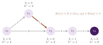
Figure 1.3, the graph of the test reopen of the library
shows the gap between the two properties. Its \(h\) is admissible, being
at most \(h^*\) on each state, but it drops by 3 along an edge of cost 1,
and A\(^*\) run on it closes \(v_2\) through the expensive edge before
finding the cheap path through \(v_1\) (the run is traced in
Chapter 2).
1.2 What makes a problem hard¶
The model of §1.1 is somewhat simple, but it contains problems that are NP-hard (e.g., the traveling salesperson problem of §14.7) and even PSPACE-complete ones (e.g., Sokoban and, in general, classical planning); hence, the form of a problem is (arguably) no indication of its difficulty. We now list the features of an instance that typically decide how hard it is for the searches of this book, in the order of section 2.3 of the textbook of Jinnai on heuristic search [164].
The size of the state space. The number of states reachable from \(s_0\)
bounds the work of a search that detects duplicates. It is \(9!/2 =
181440\) for the 8-puzzle (which the test astar checks by a
breadth-first search of the whole space), \(16!/2 \approx 1.05 \cdot
10^{13}\) for the 15-puzzle and \(25!/2 \approx 7.8 \cdot 10^{24}\) for the
24-puzzle (these counts are proved in §14.2).
An infinite state space (e.g., one with a real-valued variable) is
allowed by Definition 1.2, but then a search may not stop
when no goal is reachable.
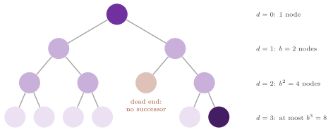
The branching factor. The branching factor of a state is the number of its successors. That of a problem is either their maximum \(b_{\max}\), which bounds the growth of a search, or their mean over the states, which is (often) what is measured and what is estimated in the literature; the two coincide on a problem whose states all have the same number of successors. A search that expands all the states up to depth \(d\) meets at most \(b_{\max}^d\) paths at depth \(d\) (Lemma 1.4 and Figure 1.4). A "large" branching factor is not in general a source of difficulty (at least, not of the kind that the parallel searches suffer from), since a dense graph also has short paths, but it multiplies the cost of each level of the search; the exact mean branching factors of the puzzles and of the grids of the library are derived in Chapter 14.
Lemma 1.4 (Paths of a given length). If each state has at most \(b_{\max}\) successors, there are at most \(b_{\max}^d\) paths of \(d\) edges that start at \(s_0\), and at most \(\sum_{k=0}^{d} b_{\max}^k\) states at distance at most \(d\) edges from \(s_0\).
Proof. By induction on \(d\): there is one path of 0 edges, and each path of \(d + 1\) edges is a path of \(d\) edges followed by one of the at most \(b_{\max}\) edges that leave its last state. Each state at distance \(k \le d\) is the last state of at least one path of \(k\) edges, which gives the second bound. \(\square\)
The bound is attained by a tree, and on a graph with duplicates the number of distinct states is usually much smaller than the number of paths; this is why the searches of this book detect duplicates.
Dead ends and irreversible actions. A problem is reversible if each action has an inverse of the same cost, as in the puzzles and the grids of unit costs, and from any state reached from \(s_0\) one can then go back to \(s_0\). In an irreversible problem (e.g., Sokoban, where a box pushed into a corner cannot be pulled back) the search may enter a region with no goal, a dead end; the searches that keep all the generated states (all those of this book but the depth-first ones) are favored there over local searches, which may spend their whole budget in such a region.
The existence of a solution. When no goal is reachable, a search that
detects duplicates proves it on a finite graph by exhausting the states
reachable from \(s_0\) (the status unsolvable of a Solution, see
§1.5). This may cost as much as the hardest solvable
instance of the same size (or more, since no goal stops the search
early), while on an infinite graph it does not stop at all. Note that
the test limits checks the first behavior on a grid split by a wall.
The n-queens problem with \(n = 2\) or \(n = 3\), or the missionaries and
cannibals with four of each and a boat of two seats, are (rather) small
unsolvable instances (§14.6).
1.3 The measures of a search¶
A search is judged by four properties, as in section 3.3 of [13]: it is complete if it returns a solution whenever one exists (and reports that none exists otherwise, when the graph is finite), optimal (or admissible) if the solution it returns has cost \(C^*\), and its time and space are the number of states it expands and the number of states it stores, as functions of the instance. For the uninformed searches these are usually given in terms of the branching factor \(b\) (the maximum \(b_{\max}\) of §1.2), the depth \(d\) of the shallowest goal, the maximum depth \(m\) of the state space and, with costs, \(C^*\) and the least edge cost \(\varepsilon\). Table 1.1 transcribes figure 3.21 of [13], which assumes a tree; the searches themselves (breadth-first, the algorithm of Dijkstra as uniform-cost search, depth-first, iterative deepening) are studied, with the proofs of these properties, in Chapter 2 and Chapter 4, and the bidirectional search in Chapter 7.
Table 1.1. Completeness, optimality, time and space of the uninformed searches on a tree (from figure 3.21 of [13]), with \(k = 1 + \lfloor C^* / \varepsilon \rfloor\): (a) complete if \(b\) is finite, (b) complete if every edge costs at least \(\varepsilon > 0\), (c) optimal if the costs are all equal, (d) with breadth-first search in both directions.
| search | complete | optimal | time | space |
|---|---|---|---|---|
| breadth-first | yes (a) | yes (c) | \(O(b^d)\) | \(O(b^d)\) |
| uniform-cost | yes (a, b) | yes | \(O(b^k)\) | \(O(b^k)\) |
| depth-first | no | no | \(O(b^m)\) | \(O(b m)\) |
| iterative deepening | yes (a) | yes (c) | \(O(b^d)\) | \(O(b d)\) |
| bidirectional | yes (a, d) | yes (c, d) | \(O(b^{d/2})\) | \(O(b^{d/2})\) |
We remark that the condition (b) is the right one on an infinite graph, and that it is not enough that the graph has no cycle of nonpositive cost. In fact, let \(s_0\) have the successors \(v_1\), at cost \(1/2\), and a goal \(t\), at cost 2, and let each \(v_i\) have the single successor \(v_{i+1}\), at cost \(2^{-(i+1)}\): the graph has no cycle at all, but \(g^*(v_i) = 1 - 2^{-i} < 1 < 2\) for every \(i\), and a uniform-cost search, which always expands a state of least \(g\), expands \(v_1, v_2, \ldots\) for ever without reaching \(t\). The next lemma is what (b) gives instead.
Lemma 1.5 (Finitely many cheap paths). On a locally finite graph whose edges all cost at least \(\varepsilon > 0\), for every \(C \ge 0\) only finitely many paths that start at \(s_0\) cost at most \(C\).
Proof. A path of \(k\) edges costs at least \(k \varepsilon\), and hence a path of cost at most \(C\) has at most \(\lfloor C / \varepsilon \rfloor\) edges. The paths of at most \(\lfloor C / \varepsilon \rfloor\) edges that start at \(s_0\) are finitely many, by the induction of Lemma 1.4 with the finite number of successors of each of the finitely many states met at each step in place of \(b_{\max}\). \(\square\)
Hence, a search that expands the states by nondecreasing \(g\) (or by nondecreasing \(f\) with an admissible \(h\)) expands finitely many states before it reaches a cost larger than \(C^*\), which is the argument of the termination theorems of Chapter 2.
The counters of a run¶
In the library, a run is measured by the counters of SearchStats
(Solution.h:73), which all the searches fill: the expansions
(expanded, including the reexpanded states, i.e., the expansions of
a state already expanded with a larger \(g\)), the generated successors
(generated), those dropped as duplicates with a \(g\) not smaller than
the known one (duplicates), the distinct states stored at the end
(stored, which Chapter 4 redefines for
IDA\(^*\), the longest path held, and for the search on the disk, the
states written to its closed files) and the wall-clock time of the
search (seconds). Thus, the
ratio generated / expanded is the mean branching factor met by the
search, usually smaller than that of the problem when the search skips
the move back to the parent (Lemma 1.8). Furthermore, a
parallel search with \(p\) workers (the threads or processes that run it,
see §1.6) records the expansions \(E_i\) of each worker \(i\)
(expanded_by) and its stored states (stored_by), and counts the
states sent to another worker (sent) and the messages that carry them
(messages). From these, the methods load_balance() and
communication_overhead() of SearchStats
(src/Solution.cpp:36 and :51) compute the load balance
as Kishimoto, Fukunaga and Botea [2] define it (on
the expansions of each worker) and the communication overhead as Jinnai and
Fukunaga [5] define it,
with the conventions that \(\mathrm{LB} = 1\) when no worker has expanded
anything or expanded_by is empty (a sequential search fills it with
one entry, which also gives \(\mathrm{LB} = 1\)) and
\(\mathrm{CO} = 0\) when nothing has been generated.
Proposition 1.6 (Range of the load balance). For \(p \ge 1\) workers, \(1 \le \mathrm{LB} \le p\); \(\mathrm{LB} = 1\) if and only if all the workers expand the same number of states, and \(\mathrm{LB} = p\) if and only if a single worker expands all of them.
Proof. With \(\Sigma = \sum_i E_i > 0\) and \(M = \max_i E_i\), one has \(\Sigma / p \le M\), since the mean of nonnegative numbers is at most their maximum, with equality if and only if they are all equal; and \(M \le \Sigma\), with equality if and only if all the other \(E_i\) are 0. Dividing by \(\Sigma / p\) gives \(1 \le \mathrm{LB} = p M / \Sigma \le p\), and the conventions above give \(\mathrm{LB} = 1\) when \(\Sigma = 0\). \(\square\)
We remark that no such bound holds in general for CO: it is at most 1 when each generated state is sent at most once, which is the case of the distributions of HDA\(^*\), but the definition does not require it. Also, the third measure of [5], the search overhead, compares the expansions of the parallel search with those of the sequential one and is computed from two runs; these measures and their use are the subject of Chapter 8 and Chapter 9.
1.4 The conventions of the pseudocode¶
The pseudocode of the book is that of the Doxygen comments of the headers, and it follows the code of the library line by line, with the following conventions (the same for the graph searches and for branch-and-bound).
- The lines are numbered, a block is given by its indentation, and the
keywords are procedure, while ... do, for each ...
do, if ... then, else, loop, return,
continue and break;
▷starts a comment. x ← eassigns,∞is the infinite cost and∅the empty set, and the relations are=,≠,<,≤,≥,∈and∉.- OPEN is the set of the generated states not yet expanded, from which a
search takes the next state to expand, and CLOSED the set of the expanded
states (in the library, the table that holds the node of each generated
state, see Chapter 2);
s₀is the initial state, andg(u),h(u),f(u) = g(u) + h(u)andparent(u)are the fields of the node of the stateu, whilec(u, v)is the cost of the edge \((u, v)\). Also,zis the incumbent, i.e., the cost of the best goal found so far (∞if none), andpis the number of workers, indexed byifrom 0 to \(p - 1\). lock Landunlock Ltake and release the lockL, andsend m to jputs the messagemin the outbox of the workerj, which may deliver it later, in a batch.- The node limits, the counters of the statistics and the prefetches are left out, since they change neither the outcome nor the order of the search.
Table 1.2 collects the notation of the book (cf. Table 1.1 of [164]), and each symbol has one meaning throughout, but for the letter \(z\), which a few chapters also use for a key of Zobrist hashing (with a subscript or an argument, \(z(s)\)).
Table 1.2. The notation of the book.
| symbol | meaning | in the library |
|---|---|---|
| \(G = (V, E)\) | the state-space graph | a Domain |
| \(s_0\) | the initial state | initial_state() |
| \(T\) | the goal states | is_goal( s ) |
| \(c(u, v)\) | the cost of the edge \((u, v)\) | c in f( t , c , h_t ) |
| \(u, v, t\) | states (nodes) | state_type |
| \(g(u)\) | cost of the best path found to \(u\) | the field g |
| \(g^*(u)\) | least cost of a path to \(u\) | |
| \(h(u)\) | heuristic estimate | heuristic( s ) |
| \(h^*(u)\) | least cost from \(u\) to a goal | |
| \(f(u)\) | \(g(u) + h(u)\), the priority of A\(^*\) | the key of OPEN |
| \(C^*\) | the optimal cost, \(h^*(s_0)\) | Solution::cost |
| \(z\) | the incumbent | the parallel searches |
| \(b\), \(d\) | branching factor, depth of a goal | |
| \(p\), \(i\) | number of workers, a worker | threads |
| OPEN | the generated, unexpanded states | OpenList.h |
| CLOSED | the expanded states | NodeTable.h |
| \(\pi\) | a solution, as a path | Solution::path |
As an example, Algorithm 1.1 is the procedure by which all the searches
of the library enumerate the successors of a state, i.e., the function
template for_each_child (Domain.h:705). Its argument o is
the operator by which u was generated (a small integer that names the
move, e.g., the cell left by the blank of a puzzle), and no_op (the
value 255, Domain.h:340) is the operator of \(s_0\), which no
move generated; when the problem knows its operators (the refinement
OperatorDomain of §1.5), the procedure passes to each
successor its own operator and skips the move back to the parent.
Algorithm 1.1 (The successors of a state).
1  procedure CHILDREN(u, h(u), o, f)   ▷ o: the operator that generated u
2     if the Domain is an OperatorDomain then
3        for each successor v of u not reached by the inverse of o do
4           f(v, c(u, v), h(v), the operator of v)
5     else
6        for each successor v of u do
7           f(v, c(u, v), h(v), no_op)
The test of line 2 is resolved at compile time (if constexpr), and
hence it costs nothing at run time; the inverse of no_op leads nowhere,
so that at \(s_0\) line 3 enumerates all the successors. The skip of line
3 is justified by Lemma 1.8 below.
1.5 The concepts of the library¶
The headers are in three layers, each with a header that includes it
whole: core.h (the helpers and the parameters of the parallel
searches, in include/PBeFS/core),
include/PBeFS/astar.h (the graph searches and
their domains, in include/PBeFS/astar) and
bnb.h (the tree searches, in include/PBeFS/bnb), while
PBeFS.h includes the three of them, save the searches over MPI.
All the searches of the library are class or function templates over the
problem, which is a type satisfying the C++20 concept Domain of
Domain.h:169 or one of its refinements; since all the calls
are resolved at compile time, the inner loop of a search pays no virtual
call, which is one of the choices of a fast implementation
recommended by Burns et al. [4]. A refinement
adds what a particular search, or a particular work distribution, needs;
hence, a problem implements only the methods required by the searches it
is meant for, and a search that needs more than the problem gives is
rejected at compile time. Both the concepts and the searches that use
them are drawn in Figure 1.5.
The concept Domain¶
A type D is a Domain (Domain.h:169) if it has
- a regular
state_type, i.e., one that is copyable and compared with==, and an arithmeticcost_type, the type of \(g\), \(h\) and the edge costs (the aliasesstate_t< D >andcost_t< D >name them); - the method
initial_state(), which gives \(s_0\), the goal testis_goal( s ), andheuristic( s ), the value \(h(s)\); - the method
hash( s ), a hash of 64 bits of the state; - the expansion
for_each_successor( s , h_s , f )of Definition 1.2, which callsf( t , c , h_t )for each successor \(t\) of \(s\), with \(c = c(s, t)\) and \(h_t = h(t)\).
The value \(h_s = h(s)\) is passed in so that one can compute \(h(t)\) incrementally from it when the heuristic allows it (e.g., the Manhattan distance of the sliding-tile puzzle, which changes by 1 at each move, see Proposition 14.5). The successors are given to a callable instead of being returned in a container, and therefore no allocation is paid per expansion.
The hash is used by CLOSED and, mixed again with a seed, by the work distribution of HDA\(^*\) that hashes the whole state (Chapter 9); with the default data structures, CLOSED takes the slot of a state from the high bits of the product of its hash by \(\lfloor 2^{64} / \phi \rfloor\), \(\phi = (1 + \sqrt5)/2\) being the golden ratio, i.e., by Fibonacci hashing (Chapter 3). The hash must therefore be "well spread", i.e., close to uniform in all its bits on the states met by a search, and no worse than that in its high bits. All the domains of the library obtain it by passing an integer image of the state to the mixing function of SplitMix64 (the addition of the constant \(\lfloor 2^{64} / \phi \rfloor\) followed by the finalizer, two rounds of an exclusive or with a right shift and a multiplication by an odd constant, and a last exclusive or with a shift). That this function spreads the bits well is an empirical property, measured by its authors and not provable in this sense; what can be proved is that it loses nothing.
Lemma 1.7 (The mixer is a bijection). The
mixing function of SplitMix64 is a bijection of the words of 64 bits.
Hence, on a domain whose hash is the mixer applied to the state itself,
a word of 64 bits (all the domains of Chapter 14
but NQueens and the puzzles of more than 16 cells), two distinct
states have distinct hashes.
Proof. The function is a composition of maps of the words of 64 bits into themselves, each of which has an inverse: the addition of a constant modulo \(2^{64}\) (inverted by its subtraction), the multiplication by an odd constant modulo \(2^{64}\) (inverted by the multiplication by its inverse modulo \(2^{64}\), which exists since the constant is coprime with 2), and \(x \mapsto x \oplus (x \gg k)\) with \(1 \le k < 64\). For the latter, the \(k\) highest bits of \(y = x \oplus (x \gg k)\) are those of \(x\), and each lower bit \(x_j = y_j \oplus x_{j+k}\) follows from a higher bit of \(x\) already known, from the top down. \(\square\)
Of course, distinct hashes may still fall in the same slot of CLOSED, whose size is much smaller than \(2^{64}\); the lemma only states that the state never loses information on its way to the hash. Nothing else is required; in particular, the concept does not require the heuristic to be admissible or consistent, which no compiler can check: the searches state in their documentation which property they need for which guarantee, and the domains of the library state which property their heuristic has (Chapter 14 proves each one).
Declaring a domain and running a search¶
The example below is compiled and run by the tester of the library (in
the case manual, ctest -R PBeFS.manual). It declares a domain whose
states are the integers from 0 to \(n\), with the moves \(s \to s + 1\) at
cost 1 and \(s \to s + 3\) at cost 2 and the goal \(n\), and it checks by a
static_assert that the type satisfies the concept. Then it calls the
function astar( domain , open , options ) of
AStar.h, i.e., the sequential A\(^*\)
of Chapter 2, with the default OPEN list (the bucket
queue for integer costs and the heap otherwise, Chapter
3) and the default options, and reads the
Solution it returns, whose fields are described below.
struct Line {

 using state_type = int;
 using cost_type = int;

 int n;                                        // the goal

 int initial_state( void ) const { return( 0 ); }
 bool is_goal( int s ) const { return( s == n ); }
 int heuristic( int s ) const { return( ( n - s ) / 3 * 2 + ( n - s ) % 3 ); }
 std::uint64_t hash( int s ) const {
  return( std::uint64_t( s ) * 0x9E3779B97F4A7C15ULL );
  }

 template< class F >
 void for_each_successor( int s , int , F && f ) const {
  if( s + 1 <= n )
   f( s + 1 , 1 , heuristic( s + 1 ) );
  if( s + 3 <= n )
   f( s + 3 , 2 , heuristic( s + 3 ) );
  }

 };

static_assert( Domain< Line > );
const auto sol = astar( Line{ 10 } );    // the bucket queue: int costs
// sol.status, sol.cost, sol.path from 0 to 10, and the counters sol.stats
The heuristic of the example is the least cost of covering the distance \(n - s\) with steps of 3 at cost 2 and of 1 at cost 1, i.e., \(2\lfloor (n - s)/3 \rfloor + (n - s) \bmod 3\). This is \(h^*\) itself, since a step of 3 is cheaper per unit and no move may pass the goal, and it is therefore consistent (\(h^*\) satisfies the inequality of Definition 1.3 by the definition of a least cost). The tester checks that the cost is 7 (three steps of 3 and one of 1), that the path goes from 0 to 10, and that A\(^*\) with \(h = 0\) gives the same cost.
The refinements¶
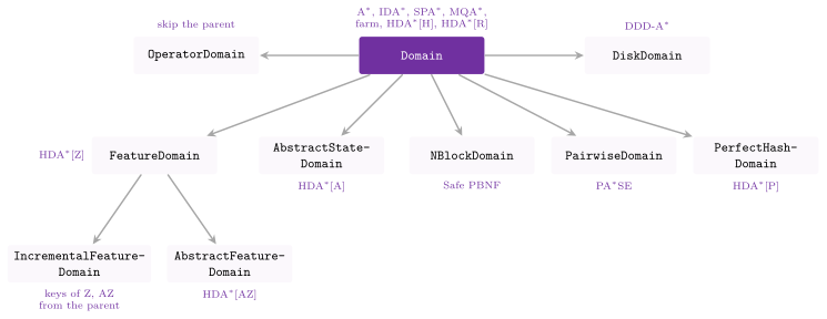
Each refinement of Domain adds a few methods, which serve the parallel
searches of the later chapters; we name each search here with one clause,
and the chapter cited gives it in full. Hash Distributed A\(^*\)
(HDA\(^*\), Chapter 9) gives each state an
owner, a worker chosen by a function of the state (its work
distribution), and sends each generated state to its owner; the
distributions are written HDA\(^*\)[Z] for Zobrist hashing, HDA\(^*\)[AZ] for
Abstract Zobrist hashing, HDA\(^*\)[P] for the perfect hash modulo \(p\), and
AHDA\(^*\) for the abstraction of the state. The Safe Parallel
Best-NBlock-First search (Chapter 11) partitions
the states into nblocks, and PA\(^*\)SE (Chapter
8) expands in parallel the states that a
pairwise heuristic proves independent. In the order of
Figure 1.5, the refinements are the following.
FeatureDomain(Domain.h:193) describes a state as a set of propositions taken from a universe ofnum_features()features, andfor_each_feature( s , f )callsf( i )for each feature \(i\) that holds in \(s\); the Zobrist hashing of HDA\(^*\)[Z] needs no more than this [2].IncrementalFeatureDomain(Domain.h:209) also gives, byfor_each_feature_change( s , t , f ), the features that hold in exactly one of \(s\) and its successor \(t\); the Zobrist key of \(t\) is then computed from that of \(s\) in as many lookups as the features that the move changes (Proposition 9.15).AbstractFeatureDomain(Domain.h:221) adds a projectionabstract_feature( i )of the features ontonum_abstract_features()abstract ones, the projection of the Abstract Zobrist hashing of HDA\(^*\)[AZ] [5].AbstractStateDomain(Domain.h:267) maps a state to an abstract state, coded as an integer byabstract_state( s ), which AHDA\(^*\) uses to keep the successors of a state on the same worker [3].NBlockDomain(Domain.h:281) partitions the state space by an abstraction intonum_nblocks()nblocks,nblock( s )being the nblock of \(s\), and enumerates byfor_each_nblock_successor( b , f )the abstract successors of the nblock \(b\), i.e., its duplicate detection scope in the Parallel Best-NBlock-First search [3]; the two conditions that the abstraction must satisfy are those of Definition 11.1.PairwiseDomain(Domain.h:295) gives a heuristicpairwise_heuristic( s , t )between any two states, which must be forward-backward consistent, as PA\(^*\)SE [6] requires.OperatorDomain(Domain.h:356) knows the operator by which a state was generated: its secondfor_each_successor( s , h_s , op , f )skips the successor reached by the inverse ofop, and passes tofthe operator of each successor (Lemma 1.8).PerfectHashDomain(Domain.h:408) gives an injective mapperfect_hash( s )of the states into the integers, which the work distribution HDA\(^*\)[P] of Burns et al. [3] reduces modulo \(p\) (see Chapter 3 for perfect hashing and Chapter 9 for its defects as a distribution).
In the searches, the operator is stored in each node, and in each message of
HDA\(^*\), through the type OperatorOf< D > (Domain.h:682),
which is an empty type when D is not an OperatorDomain; with
[[no_unique_address]] on it, a node or a message of a problem without
operators does not grow by a single byte.
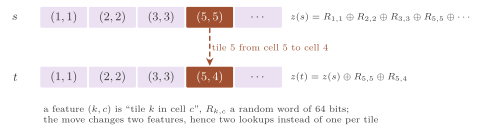
The incremental Zobrist key of IncrementalFeatureDomain rests on an
identity of the exclusive or, which Proposition
9.15 states and proves. A Zobrist key
assigns to each feature \(i\) a random word \(R_i\) of 64 bits, and to a
state \(s\) the exclusive or \(z(s) = \bigoplus_{i \in F(s)} R_i\) of the
words of the set \(F(s)\) of its features [2];
then \(z(t) = z(s) \oplus \bigoplus_{i \in \Delta} R_i\), where \(\Delta\) is
the set of the features that hold in exactly one of \(s\) and \(t\), since
the words of the features common to both appear twice and cancel. On the
sliding-tile puzzle a move changes two features (a tile leaves a cell and
enters another, Figure 1.6), and therefore the key of a
successor costs two lookups instead of one per tile; the test
hda-thread checks, on random walks of the three puzzles, that the keys
and the owners computed from the parent coincide with those computed from
scratch.
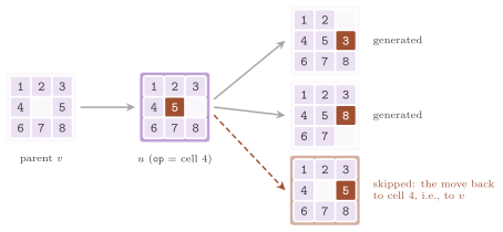
The second refinement with a statement on which the searches rely is
OperatorDomain, whose skip of the parent is one of the optimizations of
Burns et al. [4]. We prove it once for all
the searches of the library, sequential and parallel; Proposition
2.16 is its instance for A\(^*\).
Lemma 1.8 (Skipping the parent). Let an operator generate \(u\) from \(v\), and let its inverse lead from \(u\) back to \(v\) at the same cost, \(c(u, v) = c(v, u)\). In a search where the cost \(g\) of a stored state never increases, and where \(v\) stays stored once it has been expanded, assume that the current \(g(u)\), and the operator stored with it, were set when \(u\) was generated from \(v\), i.e., that \(g(u) = g(v) + c(v, u)\) for the value \(g(v)\) of that moment. Then the generation of \(v\) from \(u\) would give \(v\) a cost not smaller than its current one, i.e., it would be a duplicate that the search drops.
Proof. At the expansion of \(u\), the current cost \(g'(v)\) of \(v\) is not larger than the value \(g(v)\) it had when \(u\) was generated, since \(g\) never increases; hence, \(g(u) + c(u, v) = g(v) + 2\, c(v, u) \ge g(v) \ge g'(v)\), the costs being nonnegative. A generated state whose cost is not smaller than the known one is a duplicate: the search only counts it, and changes neither OPEN nor CLOSED. Hence, not generating it changes neither the outcome nor the order of the expansions. \(\square\)
The searches of the library that keep CLOSED never increase a \(g\) (a node is reopened only with a smaller one) and never drop an expanded state, and therefore the lemma applies to all of them, including the parallel ones, where the cost of \(v\) known at its owner is at most the cost with which \(v\) generated \(u\). The hypothesis on the cost of the inverse is not checked by the concept, and Exercise 1.3 shows what is lost without it. Among the domains of the library, the sliding-tile puzzles have operators, whose operator is the cell left by the blank (Figure 1.7), and so do the grids, the pancakes, Rubik's cube, Top Spin, the Towers of Hanoi, the permutation puzzles and the planning tasks (Chapter 14); IDA\(^*\), which has no CLOSED, prunes the parent of the other domains by comparing a successor with the state two places back on its path (Chapter 4).
The refinements of the sequential searches¶
Figure 1.5 draws the refinements by which the parallel
searches distribute their work. The sequential searches read other
refinements, which Table 1.3 lists with the searches that read them. As
above, a refinement only adds methods to Domain (or to FeatureDomain
or OperatorDomain, which it then requires); a search that does not read
it compiles and runs unchanged on a problem that offers it.
Table 1.3. The refinements of Domain read by the sequential
searches (Domain.h), the methods they add, and the searches
that read them, with the section or the chapter that describes each one.
| concept | adds | read by |
|---|---|---|
TreeOperatorDomain |
for_each_tree_successor( s , h , op , f ) |
IDA\(^*\) (§4.4) |
PartialExpansionDomain |
for_each_successor_delta( s , h , op , δ , f ) |
EPEA\(^*\) (§4.9) |
MultiHeuristicDomain |
num_heuristics(), heuristic( s , i ) |
the greedy searches (§2.12) |
PreferredDomain |
preferences( s ) |
the greedy searches, EHC (§2.12, §2.13) |
DeferredDomain |
for_each_successor_state( s , f ) |
lazy GBFS (§2.12) |
GoalFeatureDomain |
for_each_goal_feature( f ) |
SIW, BFWS (§2.15) |
RelevantFeatureDomain |
for_each_relevant_feature( s , f ) |
BFWS (§2.15) |
DistanceDomain |
distance( s ) |
the focal searches (Chapter 6) |
We describe them in the order of the table.
TreeOperatorDomainis anOperatorDomainwhosefor_each_tree_successor( s , h , op , f )gives the successors offor_each_successor( s , h , op , f )but some more. It skips those of the pairs of moves (op, then the move to the successor) that the domain declares redundant, because another pair that it keeps reaches the same state at a cost not larger; two turns of the same face of Rubik's cube, and two moves of the same disk of the Towers of Hanoi, are the examples of Korf [59]. The function templatefor_each_tree_childcalls it, and falls back onfor_each_child(Algorithm 1.1) for the other domains. The contract of the concept, which the compiler cannot check, is that every path is matched by one with the same ends, a cost not larger, and only moves that are kept. On the domains of the library a pruned pair is of one of two kinds. Either its two moves compose into one move or none (two turns of a face, two moves of a disk), and replacing them shortens the path; or they commute and come in the order that the domain does not keep (two turns of opposite faces of the cube, two commuting reversals of Top Spin), and swapping them keeps the length and lowers the number of pairs out of order. Induction on the length, and then on that number, proves the contract for them. Hence a search of the tree of the paths, which detects no duplicates, stays complete and optimal, and IDA\(^*\) reads the concept (§4.4). The searches with CLOSED do not, since the kept pair may go through a state closed with another operator, whose successors would then be pruned for good. Rubik's cube, the Towers of Hanoi, Top Spin and the permutation puzzles of the pattern databases implement it (Chapter 14).PartialExpansionDomainis anOperatorDomainwhosefor_each_successor_delta( s , h_s , op , δ , f )callsf( t , c , h_t , op_t )only for the successors \(t\) of \(s\), but the parent, whose \(\Delta f = c + h_t - h_s\) equals \(\delta\). It returns the least \(\Delta f\) larger than \(\delta\) among the others, orinfinite_cost()if there is none. This is the operator selection function of Enhanced Partial Expansion A\(^*\), which never generates a successor that it does not put in OPEN (§4.9); with real costs, \(\Delta f\) equals \(\delta\) up to the slack ofcost_slack(see below). The sliding-tile puzzles and the grids implement it.MultiHeuristicDomaingives $m = $num_heuristics()\(\ge 1\) heuristics,heuristic( s , i )being \(h_i(s)\) and \(h_0\) theheuristic( s )ofDomain. For any domain,heuristics_of( d )andheuristic_of( d , s , i )give \(m\) and \(h_i(s)\), with \(m = 1\) and \(h_0 = h\) on a domain that is not aMultiHeuristicDomain, so that the searches need not tell the two cases apart. The greedy searches alternate their queues over the heuristics, break the ties of one by another, or keep the Pareto front of their vectors [98] (§2.12). On the sliding-tile puzzles \(h_0\) is the Manhattan distance and \(h_1\) the number of misplaced tiles.PreferredDomaingives, bypreferences( s ), a predicate \(p\) computed once per expansion of \(s\), where \(p(t)\) is true if the successor \(t\) of \(s\) is preferred: e.g., the helpful actions of the planner FF [101], or the preferred operators of a heuristic [97]. The greedy searches put the preferred successors in queues of their own, while enforced hill-climbing may expand them alone or first (§2.13). On the sliding-tile puzzles a move is preferred if the tile that it moves gets closer to its goal cell, i.e., if it lowers the Manhattan distance, and on the grids if it lowers the distance to the goal.DeferredDomaingives, byfor_each_successor_state( s , f ), the successors \(t\) of \(s\) with the costs of their edges, asf( t , c ), without computing \(h(t)\). GBFS with deferred (lazy) evaluation then computes \(h\) only for the states that it selects [97], which pays when the heuristic costs far more than a move, as in planning. No domain of the library implements it, their heuristics costing no more than a move, and the testgbfswraps the 15-puzzle in one to count the evaluations.GoalFeatureDomainis aFeatureDomainwhose goal is a conjunction of features, enumerated byfor_each_goal_feature( f ): a state is a goal if and only if it has all of them. The serialized width search achieves them one at a time, and the best-first width search orders the states by the number \(\#g\) of those not yet achieved [104], [105] (§2.15). On the sliding-tile puzzles the goal features are the tiles in their goal cells, and on the grids the column and the row of the goal.RelevantFeatureDomainis aFeatureDomainwhosefor_each_relevant_feature( s , f )enumerates the features of a relaxed plan from \(s\). In the best-first width search, \(\#r\) counts the features of this set that are reached on the path to a state [105]. No domain of the library implements it, and the search then takes \(\#r = 0\).DistanceDomaingives, bydistance( s ), an estimate \(d(s)\) of the number of edges of a cheapest path from \(s\) to a goal, which need not be admissible; it is \(h\) when every edge costs 1, as on the sliding-tile puzzles. By it, the focal searches of Chapter 6 prefer the nodes closer to a goal in edges rather than in cost [52]. On the grids, whose moves cost differently, \(d\) is the number of moves to the goal on a grid without obstacles, i.e., the Manhattan distance with 4 moves and the larger of the two differences of the coordinates with 8.
Each of the other refinements of Domain.h belongs to
searches with a chapter of their own, which describes it.
BidirectionalDomain, BackwardOperatorDomain and MinCostDomain (whose
min_edge_cost() is the \(\varepsilon\) of the bounds of the bidirectional
searches) are in Chapter 7.
PredecessorDomain and EventDomain, with the events EdgeCostChanged
and GoalChanged of the incremental searches, are in
Chapter 6, and so is
BatchHeuristicDomain. EdgeDomain, LazyEdgeDomain and
HeterogeneousEdgeDomain, whose expensive_edge( s , a ) lets GePA\(^*\)SE
evaluate the cheap edges of a state together and each expensive one apart
[122], are in
Chapter 8. Last, FeatureGroupDomain and
FeatureTransitionDomain are in
Chapter 10, and LevelDomain in
Chapter 15.
Real costs¶
A cost_type may be a floating-point type, as on the grids whose
diagonal moves cost \(\sqrt 2\) times the cost of a cell. Two sums of the
same edge costs taken in another order may then differ in their last
bits, and a search that compared for equality the \(f\) of two nodes
reached along such paths would take them for different values. Hence
the searches that compare costs for equality, or test an inequality that
a rounding could reverse, allow the slack cost_slack( x , τ ) of
Node.h. It is 0 for an integer cost_type and \(\tau
\max\{1, |x|\}\) for a real one, \(\tau\) being real_cost_tolerance \(=
10^{-9}\) by default, and two values \(x\) and \(y\) are taken as equal when
\(|x - y| \le\) cost_slack( x ). The slack is relative, since the
rounding error of a sum grows with its value, and it is at least \(\tau\),
since a cost near 0 has no relative error to speak of. PEA\(^*\) and
EPEA\(^*\) use it, through the option tolerance of their
PartialOptions, and so do the selection function of the grids
(§4.9) and the test of independence of
PA\(^*\)SE (Chapter 8). Also, the largest value
of a cost_type, infinite_cost() (the infinity of a real type, the
largest integer otherwise), stands for "no path" and, as a heuristic
value, for a dead end.
We now show that the tolerance covers the paths of any practical length
for the type double, whose unit roundoff is \(u = 2^{-53} \approx 1.1
\cdot 10^{-16}\). Let \(x_1, \ldots, x_n \ge 0\) be the costs of the edges
of a path, and \(S = \sum_i x_i\). Adding them from left to right gives
\(\hat S = \sum_i x_i \prod_{j} (1 + \delta_j)\), with \(|\delta_j| \le u\),
where the product is over the at most \(n - 1\) additions that follow the
term \(x_i\). Each product lies in \([1 - \gamma_{n-1}, 1 + \gamma_{n-1}]\),
with \(\gamma_k = k u / (1 - k u)\) for \(k u < 1\) (Higham
[170],
chapters 3 and 4), and the terms are nonnegative; hence \(|\hat S - S| \le
\gamma_{n-1} S\). Two orders of the same terms thus give sums that differ
by at most \(2 \gamma_{n-1} S\), which is less than \(\tau \max\{1, S\}\) as
long as \(2 \gamma_{n-1} < \tau\), i.e., for paths of fewer than \(4 \cdot
10^6\) edges with \(\tau = 10^{-9}\). (The code compares with the computed
sum rather than with \(S\), which changes the bound by a factor \(1 +
\gamma_{n-1}\) only.) Conversely, two costs that differ by less than the
slack are taken as equal. We do not claim that this is harmless; a domain
whose distinct path costs may be that close should use integer costs, or
a smaller tolerance where the search takes one.
What a search returns¶
Every graph search returns a Solution< State , Cost >
(Solution.h:153), whose fields are those of Table 1.4; the
method solved() is true if and only if the status is solved. The values of
the enumeration Status (Solution.h:46) are solved (a
path was found, optimal under the conditions on \(h\) stated by the search),
unsolvable (OPEN emptied without reaching a goal), node_limit
(the limit of SearchOptions was reached first, see below) and
disk_limit (the limit on the bytes written to the disk was reached
first, which only the external searches of
Chapter 4 have). The field bound is a lower
bound on \(C^*\) that the search has proven, i.e., the cost itself when the
path is optimal and less than it for the searches that only bound the
suboptimality of their path, and improvements lists the paths that an
anytime search found on its way, with their costs, their bounds, the
expansions and the time at which each was found; both are described with
those searches in Chapter 6.
Table 1.4. The fields of Solution (Solution.h:153)
and their defaults; path.front() is \(s_0\) and path.back() the goal, and the
path is empty unless the status is solved.
| field | type | meaning | default |
|---|---|---|---|
status |
Status |
how the search ended | unsolvable |
cost |
Cost |
the cost of the path | Cost{} (0) |
bound |
Cost |
a proven lower bound on \(C^*\) | Cost{} (0) |
path |
vector< State > |
\(s_0\) to the goal, if solved | empty |
improvements |
vector< Improvement > |
the paths of an anytime search | empty |
stats |
SearchStats |
the counters of §1.3 | all 0 |
Next, the options shared by all the searches are those of
SearchOptions (Solution.h:188), in Table 1.5. The first
is a limit on the stored states (per worker, in a parallel search), after which
the search stops with the status node_limit; IDA\(^*\), which stores only a
path, applies it to the expansions instead, and the search on the disk
to the states written to its closed files
(Chapter 4). The second is the number of
states the search is expected to store, by which a sequential search
sizes CLOSED at the start (otherwise CLOSED is doubled, and rehashed, as
it fills); AStar reads it, and so do most of the other sequential
searches (the greedy and width-based searches of
Chapter 2, and those of
Chapter 4 that keep a table of the states),
while the parallel searches size their tables otherwise. The next four
options of the table are read by the searches that they concern. The
weight \(w\) of the heuristic orders OPEN by \(g + w h\), in the searches of
Chapter 6 and in the greedy searches of
§2.12, and the dropping of the duplicates
and the anytime search apply with a weight above 1
(Chapter 6). The goal test at the
generation of a state is made by A\(^*\) with the guarantees of
§2.11, and by the greedy searches as in
§2.12.
A search returns, as cost, the cost of the path that it found, which
is the \(g\) of the goal when the parents of the nodes of the path have not
changed since the goal was generated; when they have (a node of the path
reached later by a cheaper path, with its parent changed), the path that
the parents give is cheaper than that \(g\). The function template
path_cost( d , path ) of Domain.h gives the cost of a
path, each step taken by the cheapest edge between its two states (0 for
an empty path), and AStar returns the least of the two values; the
function check_path of test/test.h verifies, for each
search that the tester runs, that the path goes from \(s_0\) to a goal along
edges of the domain and that its cost, so computed, is the one returned.
Table 1.5. The fields of SearchOptions
(Solution.h:188) and of ParallelParams
(SearchUtils.h:98), with their defaults; 0 means "no
limit" or "unknown" in the first two; the node limit holds per worker in a
parallel search, and expected_nodes is read by the sequential searches
that keep a table of the states.
| field | type | meaning | default |
|---|---|---|---|
node_limit |
size_t |
stop after this many states | 0 |
expected_nodes |
size_t |
the states CLOSED is sized for | 0 |
weight |
double |
the weight \(w\) of \(h\) in \(g + w h\) | 1 |
drop_duplicates |
bool |
reopen only beyond what \(w\) allows | false |
anytime |
bool |
go on after the first goal | false |
goal_at_generation |
bool |
test the goal when generated | false |
threads |
unsigned |
the number \(p\) of workers | 1 |
batch |
size_t |
the states in a message | 64 |
flush_period |
unsigned |
steps between two flushes | 64 |
seed |
uint64_t |
the seed of the random draws | 1 |
1.6 Workers, executors and options of the parallel searches¶
A parallel search of the library runs \(p\) workers, indexed by
\(i = 0, \ldots, p - 1\); in shared memory each worker is a thread, and with MPI
each one is a process. In shared memory, the searches are templates over the
executor that runs their workers, i.e., a type that offers
run( p , body ), which calls body( i ) for \(i = 0, \ldots, p - 1\) at once,
each call on a separate thread, and returns when all of them have returned.
Three executors are provided: a pool of C++ threads (ThreadPool, the
default), an executor on OpenMP (OpenMPExecutor) and one on FastFlow
[12] (FastFlowExecutor); OpenMP and FastFlow are
optional dependencies, and a program can use an executor only if the library
was built with its runtime. Since the executor is a template parameter, the
same search can be compared across runtimes, and the same runtime across
searches, which the benchmarks of Chapter 8 and
Chapter 9 do.
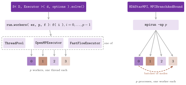
Every search starts its workers through the function
run_workers( ex , p , f ) (SearchUtils.h:125), which
is Algorithm 1.2 (Figure 1.8).
Algorithm 1.2 (Running the workers).
1  procedure RUNWORKERS(ex, p, f)
2     body ← the procedure that, given i,
3        pins its thread to the i-th CPU, unless it runs on the caller
4        calls f(i)
5     if ex ≠ ∅ then
6        ex.run(p, body)          ▷ the executor given by the program
7     else
8        E ← a new executor of p threads
9        E.run(p, body)           ▷ E is destroyed on return
Line 3 is the function pin_worker( i )
(SearchUtils.h:79): if the environment variable
PBEFS_PIN is set to a nonempty value other than 0, it binds the thread to
the \(i\)-th CPU (modulo their number) of the affinity mask of the process, where
the system allows it, and otherwise it does nothing (on a machine with several
sockets, the binding is usually needed for the timings to be repeatable). One
of the calls may run on the thread of the caller, which is left where it is.
Since run( p , body ) returns when all the calls have returned, RUNWORKERS
returns if and only if each \(f(i)\) does, and the termination of a
parallel search is that of its workers, proved search by search in the
later chapters. A program that runs many searches can give each of them
a common executor by set_executor( ex ), which saves the start of the
threads at each search (the benchmarks of the library do not use it,
and their times include that start).
The parameters of the parallel searches are those of ParallelParams
(SearchUtils.h:98, Table 1.5). Besides the number of
workers, the searches that send their states to an owner read the number of
states packed in a message and the number of steps (expansions or evaluations)
between two flushes of an outbox that is not full. The seed is that of
the random draws of the searches that make some (the queues of the
MultiQueue A\(^*\) and of several branch-and-bound schemes), while a work
distribution of HDA\(^*\) takes its own seed in its constructor. In turn,
the options of the parallel graph searches are ParallelOptions
(HDAStar.h:125), which derives from both SearchOptions and
ParallelParams and adds nothing, so that a node limit is per worker
(the expected number of states is not used by the parallel searches);
the searches with further parameters
derive their options from it (PBNFOptions in SafePBNF.h,
PASEOptions in PASE.h). The defaults of ParallelParams, 64
states per message flushed every 64 steps, are those of HDA\(^*\), and each
search sets different ones where needed. Also, its method normalize(),
which each search calls at its construction, turns threads, batch
or flush_period left at 0 into 1. Finally, the searches over MPI
(HDAStarMPI and the branch-and-bound of
MPIBranchAndBound.h) take the number of workers from
the number of processes, one worker per process; their termination detection,
which must count the messages in flight, is described in Chapter
9.
Two more helpers of SearchUtils.h serve the reproducibility
of the experiments. First, random_unit
(SearchUtils.h:157) and random_below
(SearchUtils.h:166) draw a real number in \([0, 1)\) and
an integer in \([0, n)\) directly from the words of std::mt19937_64, whose
sequence the C++ standard fixes, rather than through the distributions of
<random>, which differ between standard libraries; hence, a random grid, a
set of random cities or a random knapsack generated from a seed is the same on
all platforms. If \(x\) is the word drawn, the first returns
\(\lfloor x / 2^{11} \rfloor \cdot 2^{-53}\) and the second \(x \bmod n\), and the
next lemma states what they give when the words are uniform (an assumption on
the generator, which is only empirical).
Lemma 1.9 (The two draws). Let \(x\) be uniform on \(\{0, \ldots, 2^{64} - 1\}\). Then \(\lfloor x / 2^{11} \rfloor \cdot 2^{-53}\) is uniform on the \(2^{53}\) multiples of \(2^{-53}\) in \([0, 1)\), all exactly representable in double precision; and, for \(1 \le n \le 2^{64}\), the probability that \(x \bmod n = k\) differs from \(1/n\) by less than \(2^{-64}\) for each \(k \in \{0, \ldots, n - 1\}\).
Proof. The map \(x \mapsto \lfloor x / 2^{11} \rfloor\) takes exactly \(2^{11}\) words to each of the integers \(0, \ldots, 2^{53} - 1\), and an integer below \(2^{53}\) times a power of 2 is a double, which gives the first claim. For the second, write \(2^{64} = q n + r\) with \(0 \le r < n\): the residue \(k\) has \(q + 1\) preimages if \(k < r\) and \(q\) otherwise, and hence a probability \((q + 1)/2^{64}\) or \(q/2^{64}\); both differ from \(1/n = (q + r/n)/2^{64}\) by at most \(\max(r/n, 1 - r/n)/2^{64} < 2^{-64}\). \(\square\)
Hence, the relative bias of the second draw is less than \(n \cdot
2^{-64}\) (Lemire [151] removes it at the
price of a rejection). This is negligible for the values of \(n\) with
which the library draws, i.e., the costs of the cells of a grid (at most
255), the weights and the profits of a random knapsack, and the worker
to which a node is sent, unless the range of a knapsack is chosen close
to \(2^{64}\). Finally, Stopwatch (SearchUtils.h:176) is
the wall clock (std::chrono::steady_clock) by which the searches measure
their seconds.
1.7 The plan of the book¶
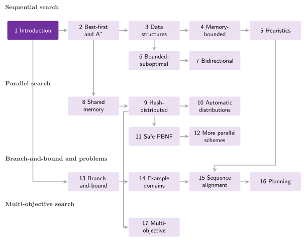
The chapters of the book and their dependencies are drawn in Figure 1.9.
- Chapter 2 gives the best-first search, its instances (breadth-first, depth-first, Dijkstra, A\(^*\)), the reopening of the closed nodes, and the properties of A\(^*\) with their proofs, i.e., completeness, optimality with an admissible heuristic, no reopening with a consistent one, and optimal efficiency, together with the goal test at the generation of a state; then the searches that give up the optimality for speed, i.e., greedy best-first search with the OPEN lists of the satisficing planners, enforced hill-climbing, the iterated searches of LAMA and the width-based searches.
- Chapter 3 treats the data structures of the searches: OPEN as a heap or as buckets, the breaking of ties, CLOSED as a hash table, perfect hashing, the arena of the nodes, and immediate against delayed duplicate detection.
- Chapter 4 treats the searches with bounded memory: beam search, depth-first branch-and-bound, iterative deepening, IDA\(^*\) and its controlled reexpansion, transposition tables, recursive best-first search, external search with delayed duplicate detection on the disk, the symbolic and novelty-based searches, partial expansion (PEA\(^*\) and EPEA\(^*\)), fringe search, the real-time searches and the hierarchical path-finding on grids.
- Chapter 5 treats the heuristics, from the relaxations to the pattern databases with their compressions, and what to do when a heuristic does not work.
- Chapter 6 gives the bounded-suboptimal searches (weighted A\(^*\) in any order of expansion, the duplicate dropping, the optimistic, focal and potential searches, the batch weighted A\(^*\)), the anytime searches (AWA\(^*\), ARA\(^*\) and the anytime parallel searches), and the incremental searches LPA\(^*\), D\(^*\) Lite and their hash-distributed versions.
- Chapter 7 gives the front-to-end bidirectional searches (the bidirectional Dijkstra, MM, fMM, BAE\(^*\), NBS, DVCBS, GBFHS), the two directions on two workers, and the parallel searches on external memory.
- Chapter 8 gives the parallel searches on a shared OPEN (SPA\(^*\), the MultiQueue A\(^*\), the farm and PA\(^*\)SE).
- Chapter 9 gives HDA\(^*\), its work distributions and the measures of §1.3, on threads and over MPI.
- Chapter 10 gives the distributions of HDA\(^*\) built from a sample of the instance, their estimates and the automatic choice among them.
- Chapter 11 gives the Safe Parallel Best-NBlock-First search.
- Chapter 12 gives the further parallel schemes: PSDD and its variants, KBFS, the portfolio of A\(^*\), PRA\(^*\), TDS, the parallel IDA\(^*\) and the parallel greedy searches.
- Chapter 13 gives branch-and-bound as a best-first search with an incumbent, and its parallel schemes.
- Chapter 14 describes the example domains of the library, with the proofs of the properties of their heuristics.
- Chapter 15 gives the multiple sequence alignment, its hyperplane work distribution, and the sets of instances of the repository.
- Chapter 16 gives classical planning as a domain of the library: the SAS\(^+\) tasks, their heuristics and the searches on them.
- Chapter 17 gives the searches whose edges cost a vector, which return the Pareto front of the paths, and their parallel versions.
1.8 Notes and references¶
The formulation of §1.1 is that of Edelkamp and Schrödl [10] (chapter 1), whose book is the reference on heuristic search, and of Russell and Norvig [13] (chapter 3), from which the measures of §1.3 and Table 1.1 are taken; the classical treatment of A\(^*\) is that of Nilsson [8], after the paper of Hart, Nilsson and Raphael [9] that introduced it, and the textbook of Jinnai [164] covers the same ground (its chapters 1 to 3) with the notation that Table 1.2 adapts. Our parallel searches follow the survey of Fukunaga et al. [1], and the measures LB and CO are those of Kishimoto, Fukunaga and Botea [2] and of Jinnai and Fukunaga [5]. Burns et al. [4] list the choices that make a search code fast (templates instead of virtual calls, a packed state, an incremental heuristic, the pruning of the parent, and so on), and the concepts of §1.5 are the way in which the library makes them available to any problem, instead of a single puzzle.
We remark that the interface of the library is narrower than that of a
general planner: a Domain exposes successors, not actions with
preconditions and effects, and therefore the domain-independent
heuristics of classical planning cannot be computed from it (this is the
subject of Chapter 16). Also, a concept checks
the signatures of the methods, not their semantics: an inadmissible
heuristic, a hash with poorly spread bits or an "inverse" operator that
costs less than the operator all compile. They then void the guarantees
of the searches; the tests of the library check the domains that it
ships (Chapter 14).
1.9 Exercises¶
Exercise 1.1 (ctest -R PBeFS.reopen). On the graph of
Figure 1.3, compute \(h^*\) and verify that \(h\) is admissible;
find every edge on which the inequality of consistency fails. Then run
A\(^*\) on it by hand, with the ties broken in favor of the larger \(g\), and
show that \(v_2\) is expanded twice, the second time with \(g(v_2) = 2\). The
test checks that the cost found is 4 and that reexpanded is positive.
Exercise 1.2 (ctest -R PBeFS.hda-thread). Prove the analogue of
the identity of Proposition 9.15 for
the Abstract Zobrist key, in which the words are indexed by the abstract
features, \(z_A(s) = \bigoplus_{i \in F(s)} R_{A(i)}\): show that the key
of a successor follows from the abstract features of the features of
\(\Delta\), and that two features of \(\Delta\) with the same abstract
feature cancel. The test checks both keys against those computed from
scratch on random walks of the 8-, 15- and 24-puzzle.
Exercise 1.3 (ctest -R PBeFS.idastar). Lemma 1.8 needs
the inverse operator to cost as much as the operator. Give a graph with
an operator whose inverse is cheaper, on which skipping the parent loses
the optimal path; then explain why comparing a successor with the state
two places back on the path (as IDA\(^*\) does on the domains without
operators) is safe on any graph with nonnegative costs. The test runs
IDA\(^*\) on the grids and on the map of Romania, which has no operators,
and checks the optimal costs.
Exercise 1.4 (ctest -R PBeFS.limits). Describe the Solution
returned by a search stopped by a node limit (its status, its cost and
its path), and the one returned on an instance with no reachable goal.
Then show that A\(^*\) on a grid of \(50 \times 50\) cells whose column 25 is
blocked expands the 1250 cells on the side of the start before it
reports unsolvable, as the test checks.
Exercise 1.5 (ctest -R PBeFS.grid). Write a wrapper Blind< D >
that satisfies Domain whenever D does and has \(h = 0\), which makes
A\(^*\) on it the algorithm of Dijkstra (see the class Blind of
test/test.cpp); explain why it does not satisfy OperatorDomain
even when D does, and what is lost by that. The test compares A\(^*\) with
and without the heuristic on random grids.
Exercise 1.6 (ctest -R PBeFS.astar). Using the counters of
§1.3, estimate the mean branching factor of the 8-puzzle met
by A\(^*\) on the instance of figure 3.28 of
[13], and explain why generated / expanded
is smaller than the mean number of moves of a state (which is derived in
Proposition 14.4). Finally, show that \(9!/2\)
states are reachable from the goal. The test checks this count by a
breadth-first search of the whole space, and A\(^*\) against the
breadth-first distances of 200 of these states; the estimate of the
branching factor is left to the reader, who can read the counters of the
runs.
Exercise 1.7 (ctest -R PBeFS.rubik). The TreeOperatorDomain of
Rubik's cube prunes, after a turn of a face, the turns of the same face
and, when that face is the second of its pair of opposite faces, the
turns of the first one. Show that a turn has 15 successors in the tree
after a turn of the first face of a pair and 12 after one of the second,
and derive the numbers 18, 243 and 3240 of the nodes at depths 1, 2 and 3
of the tree; then prove that the pruning keeps, for every path, a path
with the same ends and at most the same number of turns. The test counts
the tree to depth 5 against table 1 of Korf
[59].
Exercise 1.8 (ctest -R PBeFS.gbfs). The test wraps the 15-puzzle
in a DeferredDomain that counts the calls of its heuristic. Explain why
the greedy search with lazy evaluation on it evaluates exactly the
states that it selects and finds new, so that evaluated equals the calls
counted, and why this number is smaller than generated. What would the
same search count on the puzzle itself, which is not a DeferredDomain?
Exercise 1.9 (ctest -R PBeFS.classic). On a grid with 8 moves and
cells of real costs, give two paths from \(s_0\) to the same cell made of
the same moves in another order, and show that their costs computed in
double may differ; bound the difference as in the argument on the real
costs of §1.5, and check that cost_slack covers it for any
path of the grids of the test. The test checks that EPEA\(^*\), whose
selection function compares the values of \(\Delta f\) up to the slack,
returns the cost of A\(^*\) on such grids.