6. Bounded-suboptimal, anytime and incremental search¶
[Source: include/PBeFS/astar/Weight.h (Weight, UnitWeight,
finish_solution, settle_improvements), the fields weight,
drop_duplicates and anytime of SearchOptions and the fields bound and
improvements of Solution (Solution.h),
AnytimeAStar.h, OptimisticSearch.h,
ImprovedOptimisticSearch.h,
FocalSearch.h, PotentialSearch.h,
BatchAStar.h, LPAStar.h,
HDLPAStar.h, DynamicGraph.h, the events
of Domain.h and of Grid.h, and the weighted forms of
the searches of AStar.h, IDAStar.h,
SPAStar.h, MQAStar.h, HDAStar.h,
HDAStarMPI.h, FarmAStar.h and
SafePBNF.h]
Status — beta. The code that this chapter describes is new: it is covered by the cases
weighted,anytime,focal,lpa,batch,bounded-*andhdlpa-*of the tests, but it has not been through a release yet, and the benchmark of section 6.10 is still to be run.
We are concerned in this chapter with three families of searches that relax one of the assumptions of A\(^*\) (Chapter 2). The first gives up the optimality of the path for a bound on its cost: a search is bounded-suboptimal if, given a weight \(w \ge 1\), it returns a path that costs at most \(w\) times the optimum \(C^*\), usually after far fewer expansions than A\(^*\) needs to prove a path optimal (the classical member of the family is the weighted A\(^*\) of Pohl [46], which orders OPEN by \(g + w h\)). The second family, the anytime searches, returns a first path quickly and then improves it, together with a lower bound on \(C^*\), until the two meet or the search is stopped; the ratio of the incumbent to the lower bound bounds the suboptimality at every moment. The third family gives up the assumption that the graph is fixed: an incremental search, after the costs of some edges have changed, repairs its previous search instead of starting anew, which is the setting of the replanning of a robot that discovers its terrain as it moves [54], [143].
The three families share the machinery of this chapter, i.e., the class
Weight, which states once the rules by which a weighted search orders
OPEN, prunes with the incumbent and reopens a closed node, and the fields
of Solution that report the lower bound and the sequence of the paths
found; and the same rules make the parallel searches of Chapter
8, Chapter 9 and
Chapter 11 bounded-suboptimal and anytime. We remark
that the classical argument for weighted A\(^*\) relies on the order of the
expansions by \(g + w h\), which no parallel search follows; the rules of
Weight are therefore stated, and proved, for any order of expansion.
The structure of the chapter is as follows. Section 6.1 states the problem
and the interface common to the searches. Section 6.2 gives the class
Weight and proves that its rules keep the bound \(w C^*\) in any order of
expansion, with and without the dropping of duplicates, and section 6.3
applies them to the sequential A\(^*\) and IDA\(^*\). Section 6.4 describes the
weighted and anytime parallel searches. Section 6.5 is devoted to the anytime
searches AWA\(^*\) and ARA\(^*\) and to the anytime restarting PBNF, section 6.6
to the searches that follow a second order besides \(f\) (the optimistic
searches, the focal searches \(A^*_\epsilon\) and EES and the dynamic potential
search), and section 6.7 to the batch weighted A\(^*\). Sections 6.8 and 6.9
are concerned with the incremental searches, LPA\(^*\) and D\(^*\) Lite and their
hash-distributed version, whose correctness we prove in full. Sections 6.10
to 6.12 give the benchmark, the references and the exercises. The notation is
that of Chapter 1 and Chapter
2: \(g^*(u)\) is the cost of a cheapest path from \(s_0\)
to \(u\), \(C^*\) the cost of an optimal path to a goal (\(\infty\) if there is
none), \(f = g + h\), and \(z\) the incumbent, i.e., the cost of the best path
found so far (\(\infty\) if none).
6.1 The problem and the interface¶
We consider the problem of Chapter 1: a Domain
gives the initial state \(s_0\), the successors of a state with the costs of
the edges, the goal test and a heuristic \(h\), which is admissible unless we
say otherwise (and then \(h(t) = 0\) on every goal \(t\)). The costs are
nonnegative, and positive where a statement needs it.
Definition 6.1 (Bounded suboptimality). Let \(w \ge 1\). A search is \(w\)-admissible if, whenever a goal is reachable from \(s_0\), it returns a path to a goal of cost at most \(w C^*\). The key of a node \(n\) in a weighted search is \(f'(n) = g(n) + w h(n)\), and a lower bound \(L\) on \(C^*\) is proven by a search if \(L \le C^*\) follows from what the search has done; the ratio \(c / L\) of the cost \(c\) of a path to a proven lower bound bounds the suboptimality of that path.
Since \(h\) is admissible, \(f'(n) = g(n) + w h(n) \le w (g(n) + h(n)) = w f(n)\)
for every node, with equality when \(h(n) = 0\), e.g., on a goal; this
inequality is the one that all the proofs of this chapter use. The weight is
given to a search by the options that all the searches share
(Solution.h),
struct SearchOptions {

 /// stop with Status::node_limit after storing this many nodes (0 = no
 /// limit); IDAStar bounds the expansions instead and DDDAStar the states
 /// written to its closed files, and in a parallel search the limit holds
 /// for each worker
 std::size_t node_limit = 0;

 /// the number of nodes the search is expected to store (0 = unknown): the
 /// closed list is sized for them at the start, instead of being doubled
 /// (and rehashed) as it fills, by the searches with a closed list of their
 /// own that read it (AStar, the bidirectional and the greedy searches and
 /// most of the others)
 std::size_t expected_nodes = 0;

 /// the weight \f$ w \geq 1 \f$ of the heuristic: OPEN is ordered by
 /// \f$ f' = g + w h \f$, and the path found costs at most \f$ w C^* \f$
 /// [see Weight]; 1 is A*; the greedy searches take any \f$ w \geq 0 \f$,
 /// infinite (h alone) by default [see GreedyOptions]
 double weight = 1;

 /// with a weight above 1, a closed node reached through a cheaper path is
 /// reopened only if the saving exceeds what the weight allows, instead of
 /// always, which keeps the bound \f$ w C^* \f$ with a consistent
 /// heuristic [see Weight::improves]
 bool drop_duplicates = false;

 /// with a weight above 1, the search goes on after the first goal, the
 /// incumbent pruning the nodes by \f$ f \f$ instead of \f$ f' \f$, until
 /// it proves the incumbent optimal, recording each better path found [see
 /// Solution::improvements]
 bool anytime = false;
 /// if true, the sequential A* keeps the cheapest goal generated so far
 /// and stops as soon as no entry of OPEN has a smaller f [see AStar], and
 /// the greedy searches with eager evaluation return a goal when it is
 /// generated [see GreedyOptions]; by default the goal is tested only when
 /// a node is selected
 bool goal_at_generation = false;

 };  // end( struct( SearchOptions ) )
whose fields of this chapter are the following:
weight, the weight \(w \ge 1\) (1 by default, i.e., A\(^*\)); the searches that take it throwstd::invalid_argumentif it is below 1, and those that cannot use it (LPAStar,HDLPAStar) if it is not 1. The greedy searches take any \(w \ge 0\), with a meaning of their own (Chapter 4);drop_duplicates, which, with \(w > 1\), keeps closed a node reached through a cheaper path unless the saving exceeds what the weight allows (section 6.2);anytime, which, with \(w > 1\), makes a search go on after its first goal until it proves the incumbent optimal, recording each path that lowers it;Weightrefusesanytimetogether withdrop_duplicates, since a duplicate dropped may hold the only optimal path;goal_at_generation, which makes the sequential A\(^*\) keep the cheapest goal generated and stop as soon as no entry of OPEN has a smaller key (section 6.3).
The searches return a Solution (Solution.h), whose fields
of this chapter are
struct Improvement {
 Cost cost;                             ///< the cost of the path
 Cost bound;                            ///< the lower bound on C*
 std::uint64_t expanded;                ///< the expansions so far
 double seconds;                        ///< the time since the start
 };

Status status = Status::unsolvable;     ///< how the search ended
Cost cost{};                            ///< the cost of the path
Cost bound{};                           ///< a lower bound on C*
std::vector< State > path;              ///< the states along the path
std::vector< Improvement > improvements;  ///< the paths of an anytime
                                          ///< search, by time
SearchStats stats;                      ///< the counters of the search
The field bound is a proven lower bound on \(C^*\): the cost itself when the
path is optimal, and otherwise the bound that the weight gives (Corollary
6.6) or a better one that the search has proven, so that
cost / bound bounds the suboptimality of the path. The field
improvements lists the paths of an anytime search in the order in which
they were found, each with its cost, the lower bound known at that moment,
the expansions done so far (by the worker that found it, in a parallel
search) and the time since the start; the costs decrease strictly, and the
last one is the cost of the path returned. A search that reaches its node
limit returns Status::node_limit; an anytime search then keeps the best path
found, with the last lower bound it knows, while the other searches return
no path. The counters of SearchStats that this chapter adds are
goals_generated (the goals that improved the incumbent of
goal_at_generation when generated), iterations (the searches over the
whole graph, e.g., the iterations of ARA\(^*\)), and the counters of the
incremental searches, which we give in sections 6.8 and 6.9.
6.2 The weight and the rules of a weighted search¶
A weighted search orders OPEN by \(f' = g + w h\) in place of \(f = g + h\), and
the incumbent \(z\) prunes the nodes that cannot lead to a path the search
still looks for. Three rules decide what a search does with a node, and the
class template Weight< Cost > (Weight.h) states each of them
once, so that every search of the library applies the same ones: the
end, i.e., the condition under which no node of OPEN can lead to a path
that the search still wants; the pruning, i.e., the condition under which
the incumbent prunes a node; and the reopening, i.e., the condition under
which a node reached through a cheaper path takes the new path. The rules
depend on the mode of the search, as follows.
| mode | key | end when no node of OPEN has | pruned if | a closed node is reopened if |
|---|---|---|---|---|
| A\(^*\) (\(w = 1\)) | \(f\) | \(f < z\) | \(f \ge z\) | \(g' < g(v)\) |
| weighted | \(f'\) | \(f' < z\) | \(w f \ge z\) | \(g' < g(v)\) |
| duplicate dropping | \(f'\) | \(f' < z\) | \(f' \ge z\) | \(g(v) - g' > (w - 1)(h(u) - h(v))\) |
| anytime | \(f'\) | (OPEN empty) | \(f \ge z\) | \(g' < g(v)\) |
Here \(v\) is reached from \(u\) through a path of cost \(g'\). Note that the end
is tested on \(f'\) and the pruning on \(w f \ge f'\): a node may stay in OPEN
and yet never be expanded, which is why a worker of HDA\(^*\) drops such a node
when it reaches the top of its OPEN, rather than stopping there. With \(w = 1\)
the rules of the three weighted modes are those of the optimal searches of
Chapter 8, and Weight turns the modes off (a
search with the weight 1 is never anytime and drops no duplicate).
The interface of Weight¶
Weight is built from the weight and the two modes, or from the
SearchOptions; we quote its declarations (the bodies are in
Weight.h:104-302):
template< class Cost > class Weight {
 public:
  explicit Weight( double w = 1 , bool anytime = false , bool drop = false );
  explicit Weight( const SearchOptions & o );
  Cost key( Cost g , Cost h ) const noexcept;          // b g + a h, or g + w h
  Cost key_weighted( Cost g , Cost h ) const noexcept; // key() with w > 1
  Cost scale( Cost z ) const noexcept;                 // b z, infinity kept
  bool live( Cost k , Cost z ) const noexcept;         // k < b z, unless anytime
  bool prunes( Cost g , Cost h , Cost z ) const noexcept;
  bool prunes_weighted( Cost g , Cost h , Cost z ) const noexcept;
  template< class HU > bool improves( Cost g_old , Cost g , bool closed ,
                                      HU && h_u , Cost h_v ) const;
  Cost times( Cost f ) const noexcept;                 // floor( w f )
  Cost proven( Cost c ) const noexcept;
  Cost lower_bound( Cost c ) const noexcept;           // ceil( b c / a )
  Cost key_lower_bound( Cost k ) const noexcept;       // ceil( k / a )
  double value( void ) const noexcept;
  bool unit( void ) const noexcept;
  bool anytime( void ) const noexcept;
  bool drops( void ) const noexcept;
  };
With real costs, key( g , h ) is \(g + w h\) and the other members compare
the values that their names say. With integer costs, a key \(g + w h\) would
have to be rounded, and a rounding could change the order of two nodes or
the outcome of a test; the weight is therefore the exact fraction \(w = a / b\)
with the least \(b \le 10^4\) such that \(w b\) is an integer (to a relative
tolerance of \(10^{-9}\)), or \(\lfloor 10^4 w \rfloor / 10^4\) if there is none
(Weight.h:114-125), and the key of a node is the integer
\(b g + a h\). The weight that the search uses is value() \(= a / b\), which is
the one given when it is a fraction with a denominator up to \(10^4\) (e.g., 1.5
is \(3 / 2\) and 1.1 is \(11 / 10\)), and otherwise slightly smaller than it, so
that the bound \(w C^*\) of the given weight still holds. The keys have to fit
in the cost type, which the library does not check.
Lemma 6.2 (The integer keys). Let the costs be
integers, \(w = a / b\), and let \(f'\), \(z\) and the costs be finite. Then (i)
key( g , h ) \(= b f'\), so that the order of the keys is the order of \(f'\);
(ii) live( k , z ) holds if and only if \(f' < z\), k being the key of the
node, unless the search is anytime, when it holds for every finite key; (iii)
prunes( g , h , z ) holds if and only if \(f \ge z\) in the modes A\(^*\) and
anytime, \(f' \ge z\) with duplicate dropping and \(w f \ge z\) otherwise; (iv)
improves( g_old , g , closed , h_u , h_v ) holds if and only if
\(g < g_{\mathrm{old}}\) and, when the node is closed and duplicates are
dropped, \(g_{\mathrm{old}} - g > (w - 1)(h(u) - h(v))\); (v) for an integer
\(f'\), \(f' \le w f\) if and only if \(f' \le\) times( f ); (vi) if \(c \le w C^*\)
then \(C^* \ge\) lower_bound( c ); and (vii) if the key of some node of every
optimal path, reached with \(g = g^*\), is at least \(k\), then
\(C^* \ge\) key_lower_bound( k ).
Proof. (i) \(b g + a h = b (g + (a / b) h) = b f'\), and \(b > 0\). (ii)
scale( z ) is \(b z\), and \(b f' < b z\) if and only if \(f' < z\); an anytime
search tests only that the key is finite
(Weight.h:173-175). (iii) Without duplicate dropping the
test is \(a (g + h) \ge b z\) in 64-bit arithmetic, i.e., \((a / b) f \ge z\); with
it, the key is compared with \(b z\) as in (ii); the other modes test
\(g + h \ge z\) (Weight.h:181-202). (iv) The test
\(b (g_{\mathrm{old}} - g) > (a - b)(h(u) - h(v))\) is the stated one multiplied
by \(b > 0\), and the heuristic of \(u\) is asked for only in this case
(Weight.h:211-223), since the parent may be far away
(another worker, in HDA\(^*\) over MPI). (v) times( f ) is
\(\lfloor a f / b \rfloor\), and an integer is at most \(w f\) if and only if it
is at most its floor. (vi) \(c \le w C^* = a C^* / b\) gives \(C^* \ge b c / a\),
and since \(C^*\) is an integer, \(C^* \ge \lceil b c / a \rceil\). (vii) A node
of an optimal path with \(g = g^*\) has the key
\(b g^* + a h \le a (g^* + h) \le a C^*\), since \(b \le a\) and \(h\) is
admissible; hence \(a C^* \ge k\), and \(C^* \ge \lceil k / a \rceil\) as in
(vi). \(\square\)
The searches are written once over the rules, as templates of the weight:
UnitWeight< Cost > (Weight.h:316-346) has the
interface of Weight with the weight 1 known at compile time, its members
being static constexpr and its rules those of A\(^*\), and each search runs
its loop over UnitWeight when unit() holds and over Weight otherwise
(e.g., AStar.h:180-183). Hence, the weight costs (almost) nothing
to the optimal searches, which compile to the code they would have without
it; the members key_weighted() and prunes_weighted() serve the same
purpose inside Weight, keeping out of line what only a weight above 1
needs.
The bound in any order of expansion¶
The classical argument for weighted A\(^*\) (Theorem 6.7 below) relies on the order of the expansions by \(f'\): when the first goal is selected, its key is the least of OPEN. A parallel search does not expand in this order, and its first goal may be much worse than \(w C^*\); we therefore state the rules in a form that holds in any order, with the notion of the entries in flight of §8.3 (an entry \((u, \gamma)\) is in flight if it is in an OPEN list, held by a worker that is processing it, or in a message still to be received). A node is pruned when it is dropped without being expanded.
Proposition 6.3 (Weighted search in any order). Let \(h\) be admissible and \(w \ge 1\), and let a search, sequential or parallel, be well-formed in the sense of §8.3, except that (b) and the selection may prune a node \(n\) when \(w f(n) \ge z'\) for a value \(z'\) that \(z\) had at some earlier instant. If at an instant \(\tau\) no entry in flight that is not stale has \(f' < z\), then \(z \le w C^*\) at \(\tau\).
Proof. If no goal is reachable there is nothing to prove, \(C^*\) being infinite. Otherwise suppose that \(z > w C^*\) at \(\tau\), and let \(P = (s_0, \ldots, s_k)\) be an optimal path to a goal \(s_k\) with no goal before \(s_k\), as in the proof of Theorem 8.6. Since the search reopens every node reached through a cheaper path, the remark of that proof holds unchanged: \(g(u) \ge g^*(u)\) at every instant, the entry \((s_j, g^*(s_j))\) is created at most once, and once created it becomes stale only when this very entry is selected. Call the expansion of \(s_j\) done if a worker has selected the entry \((s_j, g^*(s_j))\) and finished processing it before \(\tau\), and let \(j\) be the least index whose expansion is not done (\(j \le k\), since a done expansion of \(s_k\) would have set \(z \le C^*\)). If \(j > 0\), the entry of \(s_{j-1}\) was selected and processed: had it been pruned, \(z \le z' \le w f(s_{j-1}) = w (g^*(s_{j-1}) + h(s_{j-1})) \le w C^*\) at \(\tau\), since \(z\) never increases; hence it was expanded, and \(s_j\) was either pruned, with \(z \le w (g^*(s_j) + h(s_j)) \le w C^*\) in the same way, or given \(g(s_j) = g^*(s_j)\) and the entry \((s_j, g^*(s_j))\). If \(j = 0\), the entry \((s_0, 0)\) is the one created at the start. In every case not yet excluded this entry exists, its expansion is not done, and it is therefore in flight at \(\tau\) and not stale, with the key
which contradicts the hypothesis. \(\square\)
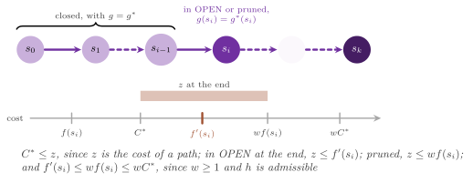
Figure 6.1 draws the proof. This is, in substance, Theorem 4 and Corollary 2 of Burns et al. ([3], section 5.1), which justify the pruning of weighted PBNF; we state it with the condition of the end, the one that a parallel search tests, and with the entries in flight, so that it covers at once all the searches of Chapter 8, Chapter 9 and Chapter 11. With \(w = 1\) it is Theorem 8.6.
Duplicate dropping¶
A weighted search reaches a closed node through a cheaper path much more often
than A\(^*\) does, and reopening it costs expansions that rarely change the path
found; the duplicate dropping variants keep such a node closed. In a
sequential weighted A\(^*\) with a consistent heuristic this keeps the bound
(Theorem 1 of Likhachev, Gordon and Thrun [48]),
but the argument relies on the order of the expansions, and a parallel search
may close a node with a \(g\) much larger than \(g^*\) before the cheaper path
arrives. The rule of Weight reopens a closed node \(v\), reached from \(u\)
with \(g' < g(v)\), only when the saving exceeds a budget that the weight
allows,
and it prunes by \(f' \ge z\) instead of \(w f \ge z\); with \(w = 1\) it reopens each node reached through a cheaper path.
Proposition 6.4 (Duplicate dropping). Let \(h\) be consistent and \(w \ge 1\), and let a search be as in Proposition 6.3, except that it reopens a closed node only as the rule above says and prunes a node \(n\) when \(f'(n) \ge z'\). If at an instant \(\tau\) no entry in flight that is not stale has \(f' < z\), then \(z \le w C^*\) at \(\tau\), in any order of expansion.
Proof. Let \(P = (s_0, \ldots, s_k)\) be as in the proof of Proposition 6.3, suppose \(z > w C^*\) at \(\tau\), and write \(D_i = \sum_{l < i} \max(0, h(s_l) - h(s_{l+1}))\) for the sum of the decreases of \(h\) along the prefix of \(P\) to \(s_i\). By the consistency of \(h\), each decrease is at most the cost of its edge, and hence \(D_i \le g^*(s_i)\). We first remark that a closed node keeps its \(g\) until it is reopened (the rule changes \(g\) only together with the reopening), and that \(g\) never increases. Let \(j\) be the least index such that \(s_j\) is not closed at \(\tau\) with its last expansion finished, or \(j = k + 1\) if there is none. We claim that for every \(i \le \min(j, k)\), from the last expansion of \(s_{i-1}\) on (from the start, for \(i = 0\)),
unless \(z \le w C^*\). For \(i = 0\), \(g(s_0) = 0\). For \(0 < i \le \min(j, k)\), \(s_{i-1}\) is closed with its last expansion done, with a value \(g(s_{i-1})\) that satisfies the claim, and that expansion offered \(g' = g(s_{i-1}) + c(s_{i-1}, s_i)\) to \(s_i\). Either it pruned \(s_i\), with
or \(s_i\) took the new path, or \(s_i\) already had \(g(s_i) \le g'\), or the saving \(g(s_i) - g'\) that \(s_i\) refused is positive and at most the budget \((w - 1)(h(s_{i-1}) - h(s_i))\); in the last three cases \(g(s_i) \le g' + (w - 1) \max(0, h(s_{i-1}) - h(s_i)) \le g^*(s_i) + (w - 1) D_i\), and \(g(s_i)\) only decreases afterwards. In the case of the pruning, \(D_{i-1} \le g^*(s_{i-1}) \le g^*(s_i)\) gives \(z \le w (g^*(s_i) + h(s_i)) \le w C^*\), against the assumption. If \(j = k + 1\), the goal \(s_k\) has been expanded, and the claim with \(D_k \le g^*(s_k) = C^*\) gives \(z \le g(s_k) \le w C^*\), a contradiction. Otherwise the claim holds for \(s_j\), which (as in Proposition 6.3) has an entry with its current \(g\) that is in flight and not stale, or was dropped at its selection by \(f'(s_j) \ge z'\); in both cases
a contradiction. \(\square\)
The proof needs the consistency of \(h\) only to bound the sum \(D_j\) of the decreases of \(h\) along the prefix of the optimal path by \(g^*(s_j)\); with an inconsistent heuristic this sum may be as large as \(j\) times \(C^*\), and the bound may fail, as the following example shows.
Example 6.5 (Duplicate dropping with an inconsistent heuristic). Let \(L \ge 1\) and \(w = 2\), and consider the graph with the edges \(s_0 \to a\), \(a \to v\), \(v \to b\) and \(b \to x\) of cost 1, \(x \to t\) of cost \(L\), and the two shortcuts \(s_0 \to v\) of cost \(5 + L\) and \(s_0 \to x\) of cost \(8 + 2L\), the goal being \(t\), and hence \(C^* = 4 + L\) along \(s_0, a, v, b, x, t\). The heuristic \(h(a) = 3 + L\), \(h(b) = 1 + L\) and \(h = 0\) elsewhere is admissible (it is exact on \(a\) and \(b\)) but not consistent. Weighted A\(^*\) with duplicate dropping expands \(s_0\), then \(v\) with \(g = 5 + L\) (key \(5 + L\), below the key \(7 + 2L\) of \(a\)), then \(a\), which offers \(g' = 2\) to the closed \(v\): the saving \(3 + L\) does not exceed the budget \((w - 1)(h(a) - h(v)) = 3 + L\), and \(v\) keeps its path. Then \(x\) is expanded with key \(8 + 2L\), before \(b\), whose key is \(6 + L + 2(1 + L) = 8 + 3L\), and the goal \(t\) is selected with \(g = 8 + 3L > w C^* = 8 + 2L\) (it ties with \(b\), and the ties go to the larger \(g\); if \(b\) were expanded first, it would offer \(7 + L\) to the closed \(x\), a saving of \(1 + L\) that the budget \(1 + L\) refuses again, and the result would be the same).
We do not know of a published rule that keeps the bound \(w C^*\) with
duplicate dropping and an inconsistent heuristic in any order of expansion;
with such a heuristic the option drop_duplicates should not be used (the
test weighted runs it on one inconsistent instance, that of the test
reopen of Chapter 2, on which the bound happens to
hold). With a consistent heuristic one has \(h(u) - h(v) \le c(u, v)\), and the
budget is at most \((w - 1) c(u, v)\), the one of the weak duplicate dropping of
Burns et al. ([3], section 5.2, Theorem 5), which
keeps the old path of \(v\) when \(g(v) \le g(u) + w c(u, v)\), i.e., when the
saving is at most \((w - 1) c(u, v)\); hence the rule of Weight reopens fewer
nodes, and it needs only the heuristic of the parent, which each node carries
(HDA\(^*\) over MPI computes it again from the state of the parent, and only
when a closed node improves). The weighted A\(^*\) that never reopens a closed
node (cf. [49], p. 357) is the special case of an
infinite budget, which keeps the bound with a consistent heuristic in the
order of \(f'\) (by the theorem of Likhachev et al. cited above), though
possibly not in an arbitrary order. In both cases the least \(f\) of OPEN is no longer a lower
bound on \(C^*\) (cf. Corollary 3 of [3]), since a
node of an optimal path may stay closed with \(g > g^*\); the bound that the
search reports is then the one of the weight.
Corollary 6.6 (The proven bounds). A search of
Proposition 6.3 or Proposition
6.4 that ends with the incumbent \(c\)
proves the lower bound proven( c ) on \(C^*\), i.e., lower_bound( c )
\(= \lceil b c / a \rceil\) with integer costs and \(c / w\) with real ones, or
\(c\) itself if it is anytime.
Proof. By the propositions, \(c \le w C^*\), and (vi) of Lemma 6.2 gives the bound. An anytime search prunes by \(f \ge z\) and ends only when no entry is in flight, which is the hypothesis of Theorem 8.6, and hence \(c = C^*\). \(\square\)
Two functions of Weight.h fill a Solution from the best goal
of a search in the same way for all the searches. finish_solution( sol ,
goal , limit_hit , h0 , w , d ) sets Status::node_limit if the node limit
was hit, and returns without a path unless the search is anytime; otherwise
it sets Status::solved (or keeps node_limit for an anytime search, whose
bound is then \(h(s_0)\), the only one that a parallel search knows without the
least \(f\) of every worker), the bound proven( g ), the path traced from the
goal and the cost. The cost is the least of \(g\) of the goal and the cost of
the path with the current parents (path_cost() of
Domain.h), which may be smaller when the path to the goal has
been improved after the goal was recorded; settle_improvements( sol ) then
appends to improvements an entry with that cost if it is below the last one
recorded, so that the last improvement is always the cost returned.
6.3 Weighted A* and weighted IDA*¶
Weighted A*¶
AStar (Chapter 2) with a weight \(w > 1\) is
weighted A\(^*\): the keys of lines 13 and 16 are those of Weight, the test of
line 14 is that of Weight::improves(), and with
SearchOptions::goal_at_generation the search keeps the goal \(\hat u\) of
least \(g\) among those generated with \(h = 0\) and stops at line 4' as soon as
no entry of OPEN has a key below \(g(\hat u)\) on the scale of the keys
(AStar.h:216-226). The pseudocode is that of
AStar.h, with the keys \(f'\):
Algorithm 6.1 (Weighted A\(^*\)).
 1  procedure A*(s₀)
 2     CLOSED ← {s₀}, with g(s₀) ← 0 and parent(s₀) ← nil
 3     OPEN ← {(f(s₀), g(s₀), s₀)}
 4'    if û exists and no entry of OPEN has f < g(û) then
          return the path to û, of cost g(û)
 4     while OPEN ≠ ∅ do
 5        (f, g, u) ← the first entry of OPEN; remove it from OPEN
 6        if u is closed or g ≠ g(u) then continue      ▷ a stale entry
 7        close u
 8        if u is a goal then return the path to u, of cost g(u)
 9        for each successor v of u do
10           g' ← g(u) + c(u, v)
11           if v ∉ CLOSED then
12              add v to CLOSED, with g(v) ← g' and parent(v) ← u
13              push (g' + h(v), g', v) in OPEN
14           else if g' < g(v) then           ▷ a cheaper path: reopen v
15              g(v) ← g';  parent(v) ← u;  v is not closed
16              push (g' + h(v), g', v) in OPEN
17     return unsolvable
Here, with a weight, \(f\) stands for \(f' = g + w h\) at lines 3, 4', 13 and 16,
and line 14 is the test of reopening of section 6.2; line 4' is executed before
line 5 at each iteration of the loop, when \(\hat u\) exists, after the stale
entries at the top of OPEN have been dropped. AStar refuses the anytime
search, which is AnytimeAStar (section 6.5), by throwing
std::invalid_argument from its constructor.
Theorem 6.7 (Weighted A\(^*\)). Let \(h\) be admissible,
\(w \ge 1\), and let a goal be reachable. Then AStar with the weight \(w\)
returns a path of cost at most \(w C^*\), with and without
goal_at_generation, and with drop_duplicates if \(h\) is consistent; its
bound is lower_bound() of that cost.
Proof. Consider an iteration of the loop before the search returns. Without duplicate dropping, Lemma 2.7 holds unchanged (its proof does not depend on the keys) and gives, on an optimal path to a goal not yet closed with \(g = C^*\), a node \(u'\) with \(g(u') = g^*(u')\) and a valid entry in OPEN of key \(f'(u') \le w (g^*(u') + h(u')) \le w C^*\). With duplicate dropping and a consistent \(h\), the claim in the proof of Proposition 6.4, applied to the first node \(s_j\) of the optimal path that is not closed, gives a valid entry of key \(f'(s_j) \le w C^*\) (or a closed goal, and the search would have returned). Hence, the least key of OPEN is at most \(w C^*\) at each iteration. A goal \(t\) selected at line 5 has \(h(t) = 0\), and its key \(g(t)\) is the least of OPEN, so that \(g(t) \le w C^*\); at line 4', \(g(\hat u)\) is at most the least key of OPEN, i.e., at most \(w C^*\), since the test failed for no smaller value. The search terminates as A\(^*\) does (Theorem 2.11), and the bound is (vi) of Lemma 6.2. \(\square\)
The order of the ties matters more with a weight than without, since many
nodes share a key \(g + w h\) while their \(f\) differ. The OPEN lists of the
library break the ties of the key in favour of the larger \(g\)
(Chapter 3); LowGOpenList< Base >
(OpenList.h) wraps a HeapOpenList and breaks them in favour
of the smaller \(g\), i.e., among the nodes of equal \(f' = g + w h\), of the
smaller \(f\), since \(f = f' - (w - 1) h\) and, among the entries of equal key,
the one of smaller \(g\) has the larger \(h\).
It pushes each entry with the \(g\) mirrored, \(M - g\) with integer costs (\(M\)
half the largest value of the type) and \(-g\) with real ones, both exact, and
mirrors it back in the entries it returns, so that the test of staleness is
unchanged. On grids this order usually expands fewer nodes and finds cheaper
paths, while the larger \(g\) is better on the sliding-tile puzzles; it is
chosen by OpenKind::heap_low_g in astar(), anytime_astar() and
optimistic_search(). A BucketOpenList cannot be its base, since it keeps
its layers dense in \(g\).
Weighted IDA*¶
IDAStar (Chapter 4) with a weight puts its
thresholds on \(f'\): each iteration explores the paths whose nodes have a key
at most the bound, the first bound being the key of \(s_0\) and the next one
the least key cut, and the root is searched only if its own key is within
the bound (IDAStar.h:185-234). The option
drop_duplicates does nothing, IDA\(^*\) having no duplicate detection, and
the constructor refuses anytime. With IDAOptions::growth above 1, the
bounds are those of IDA\(^*\)-CR of Sarkar et al.
[132], chosen by the CutoffHistogram of
Deepening.h from the histogram of the keys cut (the
DeepeningOptions of Chapter 4), and the
iteration that finds the first goal with a bound above the least key cut
before is completed as a depth-first branch-and-bound if
IDAOptions::optimal (the default), the incumbent \(z\) pruning the nodes of
\(w f \ge z\).
Proposition 6.8 (Weighted IDA\(^*\)). Let \(h\) be
admissible, \(w \ge 1\), the costs positive, and let a goal be reachable. (i)
With the classical bounds, IDAStar returns a path of cost at most \(w C^*\),
with bound equal to lower_bound() of its cost. (ii) With the bounds of
IDA\(^*\)-CR and optimal, the same holds. (iii) With the bounds of IDA\(^*\)-CR
and not optimal, the path need not be within \(w C^*\), and bound is
\(\min(c, \lceil \ell / a \rceil)\) (\(\ell / w\) with real costs), \(c\) being the
cost of the path and \(\ell\) the least key cut by the iteration before.
Proof. Every node of an optimal path \(P\), reached along \(P\), has the key
\(b g^* + a h \le a C^*\) (as in (vii) of Lemma
6.2); write \(K = \max\) of the keys along
\(P\), and hence \(K \le a C^*\). (i) Let \(\beta_k\) be the bound of the iteration
\(k\). If the iteration \(k\) finds no goal, some node of \(P\) has a key above
\(\beta_k\) (otherwise \(P\) would be explored and its goal found), the first such
node is generated and cut, and therefore \(\beta_{k+1} \le K\). Hence, either a
goal is found in an iteration whose bound is at most \(K\), or the bounds stay
at most \(K\) and increase strictly, which, the keys being of finitely many
values below \(K\) when the costs are positive (integers, or bounded away from
zero), cannot go on for ever. A goal \(t\) found with the bound \(\beta \le K\)
has \(b\, g(t) \le \beta \le a C^*\), i.e., \(g(t) \le w C^*\). (ii) The
iteration of the branch-and-bound explores every path whose keys are at most
its bound \(\beta\), pruning the nodes of \(w f \ge z\). If \(K \le \beta\), either
\(P\) is explored and its goal found, and hence \(z \le C^*\), or a node \(n\) of \(P\)
is pruned, with \(z \le w f(n) \le w C^*\). If \(K > \beta\), the goal \(t\) of the
incumbent has \(b\, g(t) \le \beta < K \le a C^*\). In both cases \(z \le w C^*\).
(iii) Every path to a goal has a node of key at least \(\ell\), since the
iteration before explored all the paths whose keys are at most its bound and
found no goal; (vii) of Lemma 6.2 gives
\(C^* \ge \lceil \ell / a \rceil\), and \(c \ge C^*\). The path itself may cost up
to the new bound, which IDA\(^*\)-CR may set far above \(K\) (cf. the bound
\(\beta_{k+1} - \ell_k\) of Deepening.h on the excess of the
first path). \(\square\)
With a weight, an iteration of IDA\(^*\) cuts the nodes whose key exceeds the
bound and therefore usually explores far fewer nodes than one on \(f\) with the
same bound; however, since the keys \(g + w h\) of the nodes are more spread out
than their \(f\), the classical bounds advance by smaller steps relative to the
size of the iterations, which is one more reason to use the bounds of
IDA\(^*\)-CR with a weight. The test weighted runs the weighted IDA\(^*\) with
\(w \in \{1, 1.5, 2, 5\}\) on the 8-puzzle, Romania and the inconsistent
instance of the test reopen (and on instances of Korf with \(w \ge 2\)).
6.4 The weighted and anytime parallel searches¶
The parallel searches of Chapter 8, Chapter
9 and Chapter 11 read
the weight and the two modes of their options (ParallelOptions and
PBNFOptions derive from SearchOptions), build a Weight from them, and
apply its rules at the lines of their pseudocode where the optimal search
tests \(f\) against \(z\); the order of the expansions changes, and the end of
the search is detected exactly as before, since the rules change only which
entries count as live. In detail:
SPAStar(§8.4) orders its OPEN by \(f'\), tests at line 7 for a node of \(f' < z\), does not expand at line 14 a node that \(z\) prunes, and prunes at lines 20 and 22 by the rule ofWeight(SPAStar.h);MQAStar(§8.6) drops at line 12 an entry popped with \(f' \ge z\) or pruned by \(z\), and expands asSPAStar(MQAStar.h);FarmAStar(§8.7) changes the tests of the master at lines 5, 8, 10 and 12 and the reopening of INSERT (FarmAStar.h);HDAStar(§9.2) orders each OPEN by \(f'\), asks at line 6 for a node of \(f' < z\), drops at line 7 the nodes that \(z\) prunes (the loop ofHDAStar.h:403-424), and prunes at lines 12 and 20 by \(w f \ge z\) (by \(f' \ge z\) with duplicate dropping, whose test of reopening replaces that of line 23);HDAStarMPI(§9.6) changes lines 8 and 9 of its pseudocode in the same way, computing the heuristic of the parent again from its state when the test of reopening needs it;SafePBNFwith a weight is the weighted PBNF (wPBNF) of section 6 of Burns et al. [3]: the OPEN lists, the values \(f(b)\) of the nblocks and the free list are ordered by \(f'\), line 8 empties OPEN(\(b\)) when its first node has \(f' \ge z\) and skips a node that \(z\) prunes, line 11 prunes the successors, line 12 reopens by the rule ofWeight, and lines 28, 30 and 60 compare \(f(b)\), now the least \(f'\) of the nblock, with \(z\) (SafePBNF.h, and Algorithm 11.1 of §11.5);PASE(§8.8) does not useWeight: its weight orders OPEN by \(g + w h\) (wPA\(^*\)SE), and its suboptimality is that of the inflation \(\varepsilon_p \ge w\) of its rule of independence, which the constructor raises to the weight; with integer costs the weight is the fraction \(a / 256\) with \(a\) rounded up, not that ofWeight.
In the anytime mode, the same searches go on after the first goal: the
incumbent prunes only by \(f \ge z\), every node of OPEN is live (in SafePBNF,
every nblock with a node stays free), and the search ends when no entry is
left in flight, i.e., with an optimal incumbent; each goal that lowers \(z\) is
appended to improvements under the lock of the incumbent, with the bound
\(h(s_0)\), since no worker knows the least \(f\) of the others. These are the
anytime weighted HDA\(^*\) and PBNF of Burns et al.
([3], section 7), and the anytime SPA\(^*\), MQA\(^*\)
and farm, which follow them.
Theorem 6.9 (The weighted parallel searches). Let \(h\)
be admissible, \(w \ge 1\), and let a goal be reachable. When SPAStar,
MQAStar, FarmAStar, HDAStar, HDAStarMPI and SafePBNF end without
reaching their node limit, (i) with the weight \(w\) the path costs at most
\(w C^*\) and bound is lower_bound() of its cost; (ii) the same holds with
drop_duplicates if \(h\) is consistent; and (iii) in the anytime mode the
path is optimal, bound is its cost, and the costs of improvements
decrease to it.
Proof. Each search is well-formed in the sense of
§8.3 up to the pruning, as the proofs of its
chapter show (§8.4 to
§8.7, §9.3,
§11.6), and its pruning is that of Weight, i.e.,
by \(w f \ge z'\), by \(f' \ge z'\) with duplicate dropping and by \(f \ge z'\) in
the anytime mode, \(z'\) being the value of the incumbent that the worker read.
Each search stops at an instant at which no entry in flight that is not stale
is live, which those proofs establish with "\(f < z\)" replaced by the test
live() of Weight, since they do not use what the test is: the counter of
MQA\(^*\), the lock of SPA\(^*\) and of the graph of SafePBNF, the master of the
farm, and the mailbox of HDA\(^*\) detect that no live entry exists, whatever
the test. Then (i) is Proposition 6.3,
(ii) is Proposition 6.4, and in (iii)
every entry is live, so that the search stops only when none is in flight and
Theorem 8.6 gives \(z = C^*\). The bounds are
those of Corollary 6.6, set by
finish_solution(), and the improvements decrease since each is recorded
under the lock only when it lowers \(z\); settle_improvements() appends the
cost of the path when it is below the last one. \(\square\)
We remark that the first path of a parallel search need not be within
\(w C^*\), nor its intermediate paths in the anytime mode, which carry only the
bound \(h(s_0)\): the guarantee is on the path returned at the end. The test
bounded-thread (and bounded-openmp, bounded-fastflow) runs the weighted,
duplicate-dropping and anytime forms of these searches with 1, 3 and 8
workers and \(w \in \{1.5, 3\}\) on two instances of Korf, a grid with 8 moves
and Romania, and the anytime restarting PBNF of section 6.5; the case mpi
does the same for HDAStarMPI.
6.5 Anytime search¶
An anytime search returns a first path quickly and then improves it, each
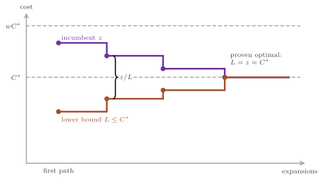
path being reported with the lower bound on \(C^*\) known when it is found, so
that the search can be stopped at any time with a path and a certified ratio
(Figure 6.2). The sequential anytime
searches are in AnytimeAStar.h:
struct AnytimeOptions : public SearchOptions {

 /// the weights of the iterations of ARA*, decreasing, the iterations
 /// after the last one having the weight 1; empty for AWA*, which keeps the
 /// weight of the SearchOptions for the whole search
 std::vector< double > schedule;

 };  // end( struct( AnytimeOptions ) )
template< Domain D , class Open = /* buckets or heap, as AStar */ >
class AnytimeAStar {
 public:
  explicit AnytimeAStar( const D & domain , const AnytimeOptions & options
                         = {} );
  [[nodiscard]] SolutionT solve( void ) const;
  };
template< Domain D > [[nodiscard]] Solution< state_t< D > , cost_t< D > >
 anytime_astar( const D & domain , const AnytimeOptions & options = {} ,
                OpenKind open = OpenKind::automatic );
With an empty schedule the search is Anytime Weighted A\(^*\) (AWA\(^*\)) of
Hansen and Zhou [47] with the weight of the
options; with a schedule it is Anytime Repairing A\(^*\) (ARA\(^*\)) of
Likhachev, Gordon and Thrun [48]. The options
drop_duplicates and anytime are not read: ARA\(^*\) has its own rule for the
closed nodes, and AWA\(^*\) reopens them to reach the optimum. The constructor
throws std::invalid_argument if a weight is below 1 or the schedule does
not decrease strictly. anytime_astar() chooses the OPEN list as astar()
does, OpenKind::heap_low_g giving the LowGOpenList of section 6.3.
Anytime weighted A*¶
AWA\(^*\) is weighted A\(^*\) that does not stop at the first goal: the incumbent
prunes by \(f \ge z\), and the search ends when OPEN is empty. A second OPEN
list FQ, ordered by \(f\), holds the same nodes, its entries becoming stale with
those of OPEN, and its least \(f\) is the lower bound reported with each path
(AnytimeAStar.h):
Algorithm 6.2 (AWA\(^*\)).
 1  procedure AWA*(s₀, w)
 2     z ← ∞;  push s₀ in OPEN (by f' = g + w h) and in FQ (by f)
 3     while OPEN ≠ ∅ do
 4        u ← the first node of OPEN, removed (stale entries dropped)
 5        if f(u) ≥ z then continue                       ▷ pruned
 6        close u
 7        if u is a goal then
 8           z ← g(u);  record (z, min(z, min f of FQ));  continue
 9        for each successor v of u with g(u) + c(u, v) + h(v) < z do
10           insert v as A* does (lines 10 to 16 of AStar.h), in OPEN
                and in FQ
11     return the path of cost z, optimal
The goal is tested when it is selected, as in AStar, whereas Algorithm 1 of
Hansen and Zhou tests it when it is generated and does not put it in OPEN; we
keep the test at the selection, so that the first goal of AWA\(^*\) is the goal
of weighted A\(^*\).
Theorem 6.10 (AWA\(^*\)). Let \(h\) be admissible,
\(w \ge 1\) and the graph finite. Then AWA\(^*\) (i) records first a path of cost
at most \(w C^*\), (ii) records with each path a lower bound
\(\min(z, \min_{\mathrm{FQ}} f) \le C^*\), (iii) records paths of strictly
decreasing costs, and (iv) ends with \(z = C^*\), bound \(= C^*\).
Proof. (i) Until the first goal, \(z = \infty\), nothing is pruned, and the search is weighted A\(^*\), whose first goal costs at most \(w C^*\) by Theorem 6.7. (ii) Before a goal of cost \(C^*\) is selected, Lemma 2.7 (whose proof holds with the pruning, since a node of an optimal path with \(g = g^*\) has \(f \le C^* < z\) and is never pruned while \(z > C^*\)) gives a node \(u'\) of an optimal path with \(g(u') = g^*(u')\) and a valid entry in OPEN, hence in FQ, of \(f \le C^*\); if \(z = C^*\) the bound is \(z\). (iii) A goal selected has \(f = g < z\) by line 5. (iv) The search is well-formed with the pruning by \(f \ge z\) and ends when OPEN is empty; Theorem 8.6 with one worker gives \(z = C^*\), and it ends on a finite graph since each node is reopened only when its \(g\) decreases, to one of finitely many values. \(\square\)
The test anytime checks (i) to (iv) with \(w \in \{1.5, 3\}\) on the 8-puzzle,
three instances of Korf, three grids with 4 and 8 moves, Romania and the
inconsistent instance of reopen. The second list doubles the entries; a
min-max heap would hold both orders in one, at the price of a slower OPEN.
Anytime repairing A*¶
ARA\(^*\) runs weighted A\(^*\) with a decreasing schedule
\(w_0 > w_1 > \cdots \ge 1\) and reuses the work of each iteration in the next.
Within an iteration no node is expanded twice: a closed node whose \(g\)
decreases goes to the list INCONS instead of OPEN, and at the end of the
iteration OPEN \(\cup\) INCONS, ordered by the next weight, is the OPEN of the
next one, CLOSED being emptied; the goal is tested when it is generated, and
\(z\) is its \(g\) (AnytimeAStar.h):
Algorithm 6.3 (ARA\(^*\)).
 1  procedure IMPROVEPATH(w)
 2     while OPEN has a node of f' < z do
 3        u ← the first node of OPEN, removed (stale entries dropped)
 4        if f(u) ≥ z then continue                       ▷ pruned
 5        close u
 6        for each successor v of u with g' = g(u) + c(u, v), g' + h(v) < z
 7           if v is new or g' < g(v) then
 8              g(v) ← g';  parent(v) ← u
 9              if v is a goal then z ← g', recording v
10              else if v is closed then add v to INCONS
11              else push (g' + w h(v), g', v) in OPEN
12  procedure ARA*(s₀, w₀, w₁, ...)
13     z ← ∞;  OPEN ← {s₀};  i ← 0
14     loop
15        IMPROVEPATH(w_i)
16        L ← min(z, min f over OPEN ∪ INCONS)
17        if z decreased in IMPROVEPATH then record (z, L)
18        if L ≥ z or OPEN ∪ INCONS = ∅ then return
19        i ← i + 1 (w_i = 1 once the schedule ends)
20        OPEN ← OPEN ∪ INCONS, by g + w_i h;  INCONS ← ∅;  CLOSED ← ∅
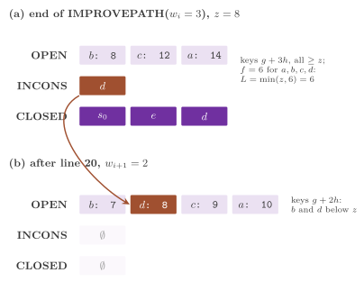
Since the OPEN lists of the library have no decrease-key, OPEN \(\cup\) INCONS is formed at line 16 by emptying OPEN, whose live entries are then pushed again with the keys of the next weight, so that no second queue is needed (Figure 6.3); the nodes closed in the iteration are kept in a list, so that line 20 opens them in time proportional to their number. A root that is a goal ends the search at once with \(z = 0\).
Lemma 6.11 (The bound of ARA\(^*\)). Let \(h\) be admissible. At line 16, \(L \le C^*\).
Proof. If no goal is reachable there is nothing to prove. Otherwise let \(P = (s_0, \ldots, s_k)\) be an optimal path to a goal, and suppose that \(z > C^*\) (otherwise \(L \le z \le C^*\)). Note that \(g\) never increases and is always the cost of a path, so that once a node has \(g = g^*\) it keeps it. Let \(j\) be the least index such that \(s_j\) has never been expanded with \(g(s_j) = g^*(s_j)\) (\(j \le k\), since the goal is never expanded). If \(j = 0\), \(s_0\) is in OPEN with \(g = 0\) (it is expanded in the first iteration otherwise, the root not being a goal). If \(j > 0\), the expansion of \(s_{j-1}\) with \(g^*(s_{j-1})\) offered \(g^*(s_j)\) to \(s_j\), which was not pruned (the test of line 6 would give \(z \le g^*(s_j) + h(s_j) \le C^*\), and \(z\) only decreases) and is not a goal before \(s_k\); hence \(s_j\) got \(g = g^*(s_j)\) then or had it already, and when it got it, it was put in OPEN or, being closed, in INCONS (or it is the goal \(s_k\), and \(z \le C^*\)). Since then, \(s_j\) has not been expanded; an entry of OPEN with \(g^*(s_j)\) is removed only by its selection, which either expands it (excluded) or prunes it by \(f(s_j) \ge z\) (excluded, as above); and line 20 moves OPEN and INCONS together into the next OPEN. Hence, at line 16, \(s_j\) is in OPEN \(\cup\) INCONS with \(f(s_j) = g^*(s_j) + h(s_j) \le C^*\), and \(L \le C^*\). \(\square\)
Theorem 6.12 (ARA\(^*\)). Let \(h\) be admissible and
the graph finite. Then ARA\(^*\) terminates, each path is recorded with a bound
\(L \le C^*\), the costs recorded decrease strictly, and the search ends with
\(z = C^*\) and bound \(= C^*\). If \(h\) is consistent, the path of the
iteration with the weight \(w_i\) costs at most \(w_i C^*\).
Proof. The bound is Lemma 6.11, and line 17 records only a \(z\) that decreased. At line 18, \(L \ge z\) gives \(z \le L \le C^*\), i.e., \(z = C^*\); an empty OPEN \(\cup\) INCONS gives \(L = z\) and the same conclusion (or no goal, \(z = \infty = C^*\)). Each iteration ends, since it expands each node at most once (a closed node goes to INCONS, not to OPEN). Once the schedule is exhausted, the iterations have the weight 1; an iteration that does not end the search leaves a node of \(f < z\) in OPEN \(\cup\) INCONS, which the next iteration, with the weight 1, either expands or prunes, and every expansion of the next iterations either lowers some \(g\) (finitely often on a finite graph, each \(g\) being the cost of one of finitely many simple paths) or empties OPEN; hence the iterations are finitely many. The last claim is Theorem 1 of Likhachev et al. [48], which holds for each call of IMPROVEPATH with a consistent heuristic, by the order of the expansions. \(\square\)
The ratio \(z / L\) of line 17 is the suboptimality \(\epsilon'\) that Likhachev
et al. report with each path ([48], section 3);
we state its bound with any admissible heuristic, while the bound \(w_i C^*\) of
each iteration needs a consistent one. The test anytime runs ARA\(^*\) with
the schedule \((w, 1 + (w - 1) / 2, 1 + (w - 1) / 4)\) on the instances of
AWA\(^*\) and checks that the first path is within \(w C^*\) and the last one
optimal, that both searches keep the best path found at the node limit, and
that a schedule that increases is refused.
Anytime restarting PBNF¶
With a nonempty PBNFOptions::schedule (the options of Chapter
11), SafePBNF is the Anytime Restarting PBNF
(ARPBNF) of Burns et al. ([3], section 7.1), i.e.,
ARA\(^*\) on the nblocks: each iteration is a wPBNF with the weight of the
schedule, which prunes by \(f \ge z\) only and keeps the nodes of \(f' \ge z\) in
OPEN for the next iterations, a closed node whose \(g\) decreases goes to the
list INCONS of its nblock, and the iteration ends at line 32 of Algorithm 11.2
(§11.5), when no nblock has a node of \(f' < z\) and
none is in use. Then the worker that finds no nblock in use, with the graph
locked, orders OPEN \(\cup\) INCONS of every nblock by the next weight, empties
the CLOSED lists, records the incumbent with the bound
\(\min(z, \min f)\) over OPEN \(\cup\) INCONS, and frees the nblocks again, until
the bound reaches \(z\) (SafePBNF.h:524-570). The
weights after the schedule are 1, and the constructor refuses a schedule
that does not decrease strictly or has a weight below 1. In the paper the
lists are ordered again at each new incumbent, with all the workers stopped
by a protocol of their own; we do it at the end of an iteration, when no
worker holds an nblock and the lock of the graph suffices. Burns et al.
report that ARPBNF improves its paths more smoothly than the anytime
weighted PBNF, but more slowly ([3], section 8.4).
Proposition 6.13 (ARPBNF). Let \(h\) be admissible and the graph finite. Then ARPBNF ends with \(z = C^*\), each path being recorded with a bound at most \(C^*\); at the node limit it keeps the best path found, with the last bound recorded.
Proof. At the end of an iteration no entry is in flight, every worker being
outside an nblock, and the argument of Lemma
6.11 applies to the union of the lists of
all the nblocks, with the pruning by \(f \ge z\) of lines 8 and 11; the end and
the termination follow as in Theorem 6.12,
each iteration being a wPBNF that ends by Theorem
11.13 and stops as in the proof of Theorem
11.12 (with the rules of Weight, as in Theorem
6.9). At the node limit the search returns
the path of its incumbent with the bound \(\min(L, z)\) of the last iteration
ended (SafePBNF.h:330-337). \(\square\)
6.6 Searches with a second order¶
Weighted A\(^*\) uses the weight both to choose the node to expand and to bound
the cost, and it is therefore often more cautious than the bound requires
(its paths usually cost much less than \(w C^*\)). The searches of this section
decouple the two: they keep a lower bound on \(C^*\), usually the least \(f\) of
OPEN, and choose the node to expand by another order, as long as the bound
allows. All of them reopen the closed nodes reached through a cheaper path,
so that the least \(f\) of OPEN is a lower bound on \(C^*\) by Lemma
2.7 (with any admissible heuristic), and all of
them read the weight of the options as the bound \(w\) and ignore anytime and
drop_duplicates.
The optimistic search¶
The optimistic search of Thayer and Ruml [49]
searches with an optimistic weight \(w_o\) larger than the bound \(w\) (by default
\(2 w - 1\), as in the paper), and then expands by \(f\) only as much as it needs
to prove that the path found is within the bound
(OptimisticSearch.h):
struct OptimisticOptions : public SearchOptions {

 /// the optimistic weight \f$ w_o \geq 1 \f$; 0 stands for \f$ 2 w - 1 \f$
 double optimism = 0;

 };  // end( struct( OptimisticOptions ) )
template< Domain D , class Open = /* buckets or heap, as AStar */ >
class OptimisticSearch {
 public:
  explicit OptimisticSearch( const D & domain ,
                             const OptimisticOptions & options = {} );
  [[nodiscard]] SolutionT solve( void ) const;
  };
template< Domain D > [[nodiscard]] Solution< state_t< D > , cost_t< D > >
 optimistic_search( const D & domain , const OptimisticOptions & options = {} ,
                    OpenKind open = OpenKind::automatic );
The search keeps the same nodes in OPEN, ordered by \(f'_o = g + w_o h\), and in FQ, ordered by \(f\):
Algorithm 6.4 (The optimistic search).
 1  procedure OPTIMISTIC(s₀, w, w_o)
 2     z ← ∞;  push s₀ in OPEN (by f'_o) and in FQ (by f)
 3     while FQ ≠ ∅ and w · (the least f of FQ) < z do
 4        if z = ∞ or OPEN has a node of f'_o < z then
 5           u ← the first node of OPEN, removed
 6        else u ← the first node of FQ, removed          ▷ the cleanup
 7        if f(u) ≥ z then continue                        ▷ pruned
 8        close u
 9        if u is a goal then z ← g(u), recording u;  continue
10        for each successor v of u with g(u) + c(u, v) + h(v) < z do
11           insert v as A* does, in OPEN and in FQ
12     return the path of cost z
The stale entries are dropped as they surface in either list, a node removed from one of them being closed, and therefore stale, in the other.
Proposition 6.14 (The optimistic search). Let \(h\) be
admissible, \(1 \le w\) and \(1 \le w_o\), and let a goal be reachable on a finite
graph. Then the optimistic search returns a path of cost at most \(w C^*\),
with bound \(= \min(z, \min_{\mathrm{FQ}} f) \le C^*\), whatever \(w_o\); each
path that lowers \(z\) is recorded in improvements with the least \(f\) of FQ
at that moment.
Proof. As in the proof of Theorem 6.10, while \(z > C^*\) a node of an optimal path with \(g = g^*\) and \(f \le C^*\) has a valid entry in FQ (it is never pruned, since \(f \le C^* < z\), and it leaves FQ only by its expansion, which puts the next node of the path in its place), so that the least \(f\) of FQ is at most \(C^*\); if \(z \le C^*\) the bound is \(z\). The loop ends at line 3 either when FQ is empty, and then no node of \(f < z\) is left and \(z = C^*\) by Theorem 8.6 with one worker, or when \(w \min_{\mathrm{FQ}} f \ge z\), which gives \(z \le w \min_{\mathrm{FQ}} f \le w C^*\). It ends, since every iteration either removes a stale entry or closes a node with a new value of \(g\), which happens finitely often. The order of line 4 changes neither argument, and \(w_o\) decides only how soon the bound is reached. \(\square\)
The test of line 3 is prunes( f , 0 , z ) of a Weight without modes, i.e.,
\(w \min f \ge z\) exactly with integer costs. If the first path is already
within the bound when it is found, the search ends without any cleanup; if
not, the cleanup expands the nodes of least \(f\) until the least \(f\) of FQ
rises to \(z / w\), possibly finding cheaper goals on the way (the "optimistic"
bet of the paper is that it seldom needs many).
The improved optimistic search¶
The Improved Optimistic Search (IOS) of Chen, Sturtevant, Doyle and Ruml
[50] adds two ideas to the optimistic search:
a lower bound gathered by the first search, and the solution update, which
lowers the incumbent when a cheaper path to a node of the incumbent path is
found, without expanding that path again. In
ImprovedOptimisticSearch.h, with the options
of OptimisticSearch, \(z\) the cost of the first path \(P\), \(r\) the largest
saving found on a node of \(P\) and \(L\) the lower bound:
Algorithm 6.5 (IOS).
 1  procedure IOS(s₀, w, w_o)
 2     L ← 0;  weighted A* by g + w_o h, no closed node reopened, each
          node selected raising L to (g + w_o h) / w_o, until a goal is
          selected:  z ← its g, P ← its path
 3     every node is closed;  r ← 0;  push s₀ in OPEN by f
 4     while OPEN ≠ ∅ and z − r > w L do
 5        u ← the first node of OPEN by f, removed;  L ← max(L, f(u))
 6        close u;  if u is a goal then z ← g(u);  r ← 0;  P ← its path;
             break
 7        for each successor v of u, with g' = g(u) + c(u, v) do
 8           if v ∈ P and g' < its g on P then r ← max(r, its g on P − g')
 9           if v was not reached since line 3 then
10              g(v) ← g';  parent(v) ← u;  push v in OPEN     ▷ reopened
11           else insert v as A* does
12     return P improved by r, of cost z − r
The path of line 12 is the one to the node of \(P\) with the saving \(r\), followed by the rest of \(P\), which is the solution-update policy of the paper; if no saving was found, \(P\) itself is returned, since the second search may have given its nodes other parents. Algorithm 1 of the paper goes on instead from the OPEN of the first search, ordered by \(f\), with no reopening, and proves the bound also by its least \(f\); we restart from the root because, when the closed nodes are not reopened, a node of an optimal path may stay with \(g > g^*\), and the least \(f\) of OPEN is then not a lower bound on \(C^*\) (cf. Corollary 3 of [3]). The two phases are not interleaved, as in the configuration that the paper recommends.
Proposition 6.15 (IOS). Let \(h\) be consistent,
\(w, w_o \ge 1\), and let a goal be reachable on a finite graph. Then IOS
returns a path of cost at most \(w C^*\), with bound \(= \min(L, z - r)
\le C^*\).
Proof. The first search is a weighted A\(^*\) with the weight \(w_o\) and no reopening; with a consistent heuristic every node it selects before its goal has \(g + w_o h \le w_o C^*\) (Theorem 1 of Likhachev et al. [48], the first iteration of ARA\(^*\)), so that the \(L\) of line 2 is at most \(C^*\); with integer costs it is the key divided by \(a\) and rounded up, \(\lceil (b g + a h) / a \rceil\), still at most \(C^*\). The second search is an A\(^*\) from the root with reopening: line 9 treats a node of the first search as new the first time it is reached, and line 11 reopens it afterwards, so that Lemma 2.8 applies, every node it selects before a goal has \(f \le C^*\), and the \(L\) of line 5 stays at most \(C^*\); a goal selected at line 6 is optimal. The value \(z - r\) is the cost of a path (the path to the node \(v\) of \(P\) with the saving \(r\), of cost \(g'\), and the rest of \(P\), of cost \(z - g_P(v)\)). The loop ends by line 6, by an empty OPEN (and then the A\(^*\) has expanded every node of \(f < z - r\), so that \(z - r = C^*\)), or by \(z - r \le w L \le w C^*\). \(\square\)
The consistency is needed by the first phase only. The test focal runs IOS
only on the instances with a consistent heuristic, among them three states of
the 8-puzzle whose first path the second search reaches anew, giving its
nodes other parents.
The focal searches¶
The focal search \(A^*_\epsilon\) of Pearl and Kim [51]
expands, among the nodes of OPEN with \(f \le w f_{\min}\) (the list FOCAL),
the one that a second order prefers, \(f_{\min}\) being the least \(f\) of OPEN.
Explicit Estimation Search (EES) of Thayer and Ruml
[52] orders the focal list by an inadmissible
estimate \(\hat d\) of the distance to a goal in edges, built from estimates
corrected online, and chooses among three lists. Both are in
FocalSearch.h:
enum class FocalOrder {
 distance ,    ///< the distance d of a DistanceDomain, h otherwise
 heuristic ,   ///< h
 optimistic ,  ///< \f$ g + ( 2 w - 1 ) h \f$
 explicit_estimation   ///< EES, with \f$ \hat d \f$ and three lists
 };
struct FocalOptions : public SearchOptions {

 FocalOrder order = FocalOrder::distance;     ///< the order of FOCAL

 };  // end( struct( FocalOptions ) )
template< Domain D > class FocalSearch {
 public:
  explicit FocalSearch( const D & domain , const FocalOptions & options = {} );
  [[nodiscard]] SolutionT solve( void ) const;
  };
The order distance is the distance \(d\) of a DistanceDomain
(Domain.h), i.e., the estimate distance( s ) of the number of
edges to a goal, which need not be admissible and is \(h\) when every edge costs
1; on another domain it is \(h\). The order heuristic is \(h\), the order
optimistic is \(g + (2 w - 1) h\), and explicit_estimation is EES. In the
focal search, with \(k\) the second order:
Algorithm 6.6 (The focal search \(A^*_\epsilon\)).
 1  procedure FOCAL(s₀, w)
 2     OPEN ← {s₀};  B ← w f(s₀);  FOCAL ← {s₀}
 3     while OPEN ≠ ∅ do
 4        B' ← w f_min
 5        if B' > B then move to FOCAL the nodes of OPEN with B < f ≤ B'
 6        B ← B'
 7        u ← the first node of FOCAL by k, removed
 8        if f(u) > B then put u back among the nodes not in FOCAL;
             continue
 9        close u;  if u is a goal then return its path
10        for each successor v of u, inserted as A* does, put v also in
             FOCAL if f(v) ≤ B
OPEN is kept by \(f\), with the nodes not in FOCAL also in a list PENDING by
\(f\), from which line 5 takes them in order; the three lists are LazyQueues,
heaps of nodes by a key of any type (then by the larger \(g\)) that drop their
stale entries lazily as the OPEN lists do, each entry carrying a second value
read back with it (FocalSearch.h). Line 8 handles a
\(f_{\min}\) that decreases, which only an inconsistent heuristic causes (a node
reopened with a smaller \(f\)). With integer costs, \(B = \lfloor w f_{\min}
\rfloor\) (times() of Weight), which compares exactly by (v) of Lemma
6.2.
EES keeps OPEN by \(\hat f = g + \hat h\), FOCAL with the nodes of
\(\hat f \le w \hat f_{\min}\) by \(\hat d\), and CLEANUP by \(f\). The estimates
are corrected online by the mean one-step errors \(\bar\epsilon_h\) and
\(\bar\epsilon_d\), measured at each expansion on the best child (that of least
\(c + h\)): \(\epsilon_h = c(u, v) + h(v) - h(u)\),
\(\epsilon_d = 1 + d(v) - d(u)\), \(\hat d = d / (1 - \bar\epsilon_d)\) and
\(\hat h = h + \bar\epsilon_h \hat d\) (section 3 of
[52]), with the values when the node is inserted;
\(\bar\epsilon_d\) is clamped to \([0, 1 - 10^{-6}]\) and \(\bar\epsilon_h\) to
nonnegative values (FocalSearch.h:410-420). FOCAL is
kept as in the focal search, on \(\hat f\) in place of \(f\), and the node to
expand is chosen by
Algorithm 6.7 (EES: the choice of the node).
 1  procedure SELECTNODE()
 2     b_d ← the first node of FOCAL;  b_f̂ ← that of OPEN;
       b_f ← that of CLEANUP
 3     if f̂(b_d) ≤ w f(b_f) then return b_d
 4     if f̂(b_f̂) ≤ w f(b_f) then return b_f̂
 5     return b_f
Proposition 6.16 (The focal searches). Let \(h\) be
admissible, \(w \ge 1\), and let a goal be reachable on a finite graph. Then
FocalSearch returns a path of cost at most \(w C^*\) with every order, with
bound \(= \min(f_{\min}, g)\) at the selection of the goal, whatever the
distance of a DistanceDomain.
Proof. By the reopening, the least \(f\) of OPEN (or of CLEANUP, in EES) is at most \(C^*\) at each iteration (Lemma 2.7). In the focal search, every node of OPEN with \(f \le B\) is in FOCAL, including the node of \(f_{\min}\) (the nodes of PENDING have \(f > B\), since line 5 moves those below \(B\) when \(B\) rises, and line 8 puts back only those above it when \(B\) falls), so that FOCAL is not empty at line 7, and a node expanded at line 9 has \(f \le B = w f_{\min}\); a goal \(t\) has \(h(t) = 0\), hence \(g(t) = f(t) \le w f_{\min} \le w C^*\). In EES the corrections are nonnegative (\(\bar\epsilon_h\) is taken as 0 when negative, and \(\hat d \ge 0\)), and hence \(\hat f \ge f \ge g\) for every node, whatever the errors; a goal returned at line 3 or 4 has \(g \le \hat f \le w f(b_f) \le w C^*\), and one returned at line 5 has the least \(f\) of CLEANUP, i.e., it is optimal. The search ends, since each iteration closes a node with a new value of \(g\) or moves an entry between the lists a bounded number of times. \(\square\)
The estimates of EES change only the order, never the bound; on a goal
\(h = 0\) and, if the distance of the domain is 0 there too, \(\hat f = g\), as in
the paper. The orders of FocalSearch that ignore the cost (\(d\) and \(h\)) are
those of the original \(A^*_\epsilon\), and they may expand many more nodes than
weighted A\(^*\) when the nodes of small \(d\) are expensive, which is the
weakness of \(A^*_\epsilon\) that motivated EES
([52], section 2).
The dynamic potential search¶
The Dynamic Potential Search (DPS) of Gilon, Felner and Stern [53] has no parameter but the bound: it expands the node of OPEN of largest potential
i.e., the node most likely to lead to a path of cost at most \(w f_{\min}\) if
the relative error of \(h\) is uniform. A node of \(h(n) = 0\) is given
\(h = 10^{-30}\), so that it comes before all the others if
\(g(n) < w f_{\min}\) and after all of them if \(g(n) > w f_{\min}\), and among
the nodes of \(h = 0\) the one of larger \(w f_{\min} - g(n)\) comes first
(PotentialSearch.h):
template< Domain D > class PotentialSearch {
 public:
  explicit PotentialSearch( const D & domain ,
                            const SearchOptions & options = {} );
  [[nodiscard]] SolutionT solve( void ) const;
  };
Algorithm 6.8 (DPS).
 1  procedure DPS(s₀, w)
 2     OPEN ← {s₀};  F ← f(s₀)
 3     while OPEN ≠ ∅ do
 4        if f_min ≠ F then F ← f_min;  order OPEN again by ud
 5        u ← the node of OPEN of largest ud, removed
 6        close u;  if u is a goal then return its path
 7        insert the successors of u as A* does, by ud
OPEN is kept twice, by \(f\) for \(f_{\min}\) and by ud in a heap rebuilt at line
4 from its live entries, both LazyQueues.
Proposition 6.17 (DPS). Let \(h\) be admissible,
\(w \ge 1\), and let a goal be reachable on a finite graph. Then DPS returns a
path of cost at most \(\max(w f_{\min}, C^*) \le w C^*\), \(f_{\min}\) being taken
at the selection of the goal, with bound \(= \min(f_{\min}, g)\), provided
that the factor \(10^{30}\) separates the potentials of the nodes of \(h = 0\)
from the others (which holds unless the costs or \(h\) are below \(10^{-30}\)
relative to \(w f_{\min}\)).
Proof. By the reopening, OPEN holds a node \(n\) of an optimal path with \(g(n) = g^*(n)\), and \(f_{\min} \le f(n) \le C^*\). Let \(t\) be the goal selected. If \(g(t) \le w f_{\min}\) we are done. Otherwise its potential is negative and, \(h(t)\) being 0, below that of every node of \(h > 0\); since \(t\) has the largest potential, every node of OPEN has \(h = 0\), in particular \(n\), and the order among the nodes of \(h = 0\) gives \(w f_{\min} - g(n) \le w f_{\min} - g(t)\), i.e., \(g(t) \le g^*(n) = g^*(n) + h(n) \le C^*\). \(\square\)
The paper gives every node of \(h = 0\) an infinite potential (footnotes 4 and 6 of [53]), which would expand first a goal of \(g > w f_{\min}\); the order above keeps the bound in this case too. The rebuild of line 4 costs \(O(|\mathrm{OPEN}| \log |\mathrm{OPEN}|)\) once for each value of \(f_{\min}\), which with integer costs and a consistent heuristic are at most \(C^* - h(s_0) + 1\); the paper keeps OPEN in buckets of equal \(g\) and \(h\) and orders only the buckets (section 4.2), which we have not implemented.
6.7 Batch weighted A*¶
When the heuristic is a learned function evaluated on an accelerator, its cost
per state falls steeply with the number of states evaluated at once, and a
search that computes it one state at a time wastes the accelerator. The batch
weighted A\(^*\) by which Agostinelli et al. [126]
search with a learned heuristic takes the \(K\) best nodes of OPEN at each
cycle, expands them all, and computes the heuristic of their new successors in
one call; it orders OPEN by \(g + w h\) (written there \(\lambda g + h\), i.e.,
\(w = 1 / \lambda\)). In BatchAStar.h:
struct BatchOptions : public SearchOptions {

 /// the nodes expanded at each cycle, 1 if 0
 std::size_t batch = 1;

 };  // end( struct( BatchOptions ) )
template< Domain D , class Open = /* buckets or heap, as AStar */ >
class BatchAStar {
 public:
  explicit BatchAStar( const D & domain , const BatchOptions & options = {} );
  [[nodiscard]] SolutionT solve( void ) const;
  };
template< Domain D > [[nodiscard]] Solution< state_t< D > , cost_t< D > >
 batch_astar( const D & domain , const BatchOptions & options = {} );
A batch of 0 is taken as 1, and a weight below 1 as 1. The heuristic is
computed in batches when the domain models the concept BatchHeuristicDomain
of Domain.h, i.e., provides
heuristic_batch( s , h ), which writes in h[ i ] the heuristic of the
state s[ i ] for two spans of equal size; the search then ignores the \(h\)
that for_each_successor passes with each successor, which may be 0. A node
keeps \(w h\) in its field h, rounded down with integer costs, so that the
OPEN lists of A\(^*\) order by \(g + w h\) unchanged:
Algorithm 6.9 (Batch weighted A\(^*\)).
 1  procedure BATCHA*(s₀, K, w)
 2     CLOSED ← {s₀};  OPEN ← {(g(s₀) + w h(s₀), s₀)};  z ← ∞
 3     while OPEN has a node of f < z do
 4        B ← the (at most) K first nodes of OPEN of f < z, removed
 5        N ← ∅
 6        for each u ∈ B, closed, do
 7           if u is a goal then z ← min(z, g(u)), recording u;  continue
 8           for each successor v of u, g' ← g(u) + c(u, v) do
 9              if v ∉ CLOSED then add v to CLOSED and to N
10              else if g' < g(v) then v is not closed
11              else continue
12              g(v) ← g';  parent(v) ← u
13        compute h(v) for all the v ∈ N at once
14        push in OPEN the nodes of lines 9 and 10 of f < z
15     return the path to the goal of cost z, if z < ∞
Here \(f\) stands for \(g + w h\). Line 13 calls heuristic_batch() once per
cycle, on the new states only (a duplicate keeps the \(h\) it has); on another
domain the \(h\) passed with the successors is used, the search asking the
domain for the true heuristic of the parent when \(w > 1\), since the field h
holds \(w h\). Line 14 pushes the nodes in the order in which A\(^*\) would have
pushed them.
Proposition 6.18 (Batch weighted A\(^*\)). Let \(h\) be
admissible, \(w \ge 1\), \(K \ge 1\), and let a goal be reachable on a finite
graph. Then BatchAStar returns a path of cost at most \(w C^*\), optimal if
\(w = 1\), whatever \(K\); with \(K = 1\) it is A\(^*\) with the heuristic
\(\lfloor w h \rfloor\) (or \(w h\)), and with \(w = 1\) and \(K = 1\) it expands
the nodes of AStar, in the same order.
Proof. The search is well-formed in the sense of
§8.3 with one worker, the batch being the
entries held: it reopens the nodes reached through a cheaper path (line 10),
records every goal it selects, and prunes a node when its key \(g + w h\), which
is at most \(w f\), is not below \(z\) (lines 3, 4 and 14). It stops when no node
of OPEN has a key below \(z\) and no batch is held, and the argument of
Proposition 6.3 applies, with the key of
the node of the optimal path at most \(w C^*\) (and \(\lfloor w h \rfloor \le w
h\)); with \(w = 1\) it is Theorem 8.6. With
\(K = 1\) each cycle expands the first node of OPEN, and a goal selected sets
\(z\) to its key, which no node of OPEN is below, so that the loop ends: this is
A\(^*\) with the heuristic of the keys, line 14 pushing the successors in the
order of AStar. \(\square\)
With \(K > 1\) a goal may be selected together with nodes of smaller key, whose
expansions may still lead to a cheaper goal, which is why a goal does not stop
the search at once; a larger \(K\) expands more nodes, those of the last batch
beyond the optimum, but calls the heuristic \(K\) times less often. The search
leaves Solution::bound at 0 (it proves no bound) and records no
improvement. The test batch checks that \(K = 1\) expands the nodes of A\(^*\)
on easy instances of Korf, that \(K \in \{8, 64, 512\}\) keeps the optimal cost,
that \(K = 64\) with \(w = 2\) stays within \(2 C^*\), and, on a domain of the test
that models BatchHeuristicDomain, that the heuristic is computed exactly
once per state stored, in at most one call per 32 expansions with \(K = 64\).
6.8 Incremental search¶
The changes of a domain¶
An incremental search keeps its work between two searches on a domain whose
edges and goals change in between. The domain has to give the predecessors of
a state, i.e., to model the concept PredecessorDomain of
Domain.h (for_each_predecessor( s , f ) calls f( t , c ) for
every state \(t\) with an edge \((t, s)\) of cost \(c\), the edges being those that
for_each_successor() gives at the same time), and the changes are told to the
search as events:
template< class State , class Cost > struct EdgeCostChanged {
  State u;  State v;  Cost from;  Cost to;      // the edge ( u , v ), costs
  };
template< class State > struct GoalChanged {
  State t;  bool added;                         // t became a goal, or not
  };
enum class CostChanges { increase_only , decrease_only , both };
template< class D > concept EventDomain;          // PredecessorDomain, and
                                                  // d.drain_events( f )
template< class D > constexpr CostChanges cost_changes_of( void ) noexcept;
An absent edge costs \(\infty\) (infinite_cost()), so that an edge that appears
is a change from \(\infty\) and one that disappears a change to \(\infty\), and a
state blocked or freed is the change of each edge into it and out of it (as in
Ramalingam and Reps [144]). The old cost is in the
event because the domain no longer knows it, and because the repair treats a
decrease in \(O(1)\) and an increase only when the edge was the one of the
parent (see below). An EventDomain gives, by drain_events( f ), the events
since the last call, an EdgeCostChanged or a GoalChanged each, and forgets
them; the events of one edge are coalesced into one, from the cost before the
first change to the cost after the last, and those that change nothing are
dropped. A domain may declare the static member cost_changes, of type
CostChanges, which cost_changes_of< D >() returns (both if there is none),
so that an incremental search compiles out the repair of the direction that
never happens and refuses the changes of that direction. The heuristic must
stay consistent for every cost that the edges take.
Two domains of the library are event domains. DynamicGraph< Cost >
(DynamicGraph.h) is a directed graph on the nodes
\(0, \ldots, n - 1\) whose arcs change their costs (set_cost( e , c ), the arcs
being numbered in the order of add_edge()), whose nodes are blocked and freed
(set_blocked(), an arc with a blocked end being absent) and whose goals
change (set_goal()); the heuristic is the Manhattan distance to the nearest
goal times set_scale() if the nodes have positions (set_position()), or a
value per node given by set_heuristic(), and since an incremental search
computes the \(h\) of a state once, a set of goals that changes under the
Manhattan distances needs the fixed set of set_heuristic_goals(), the
union of the goals of every search, and hence \(h\) stays consistent and 0 on the
goals of each of them. grid( w , h , c ) builds a four-connected gridworld,
and gridworld( w , block , gen ) and perturb( frac , blocks , gen ) the
gridworlds of the experiments of Koenig, Likhachev and Furcy
([54], section 7) and their changes: \(51 \times
51\) cells, the arcs of cost 1 or 2 drawn uniformly and a fraction of them
redrawn after each search (their figure 8), or the cells blocked with
probability 0.2 and some of them blocked and freed after each search (their
figure 9). The grids of Grid.h (Chapter 14)
are event domains as well: after a change of the cost of a cell by
GridMap::set_cost(), Grid::cell_changed( x , y , old ) patches the moves
around the cell and records the change of each move between two of the
\(3 \times 3\) cells around it, the only ones that the cell can change (its own,
those into it and the diagonals that cut it), and drain_events() hands them
to the search; the heuristic must stay admissible as for Grid::refresh(),
i.e., the new costs of the free cells must not go below the smallest cost of
the map when the grid was built.
Lifelong planning A*¶
Lifelong Planning A\(^*\) (LPA\(^*\)) of Koenig, Likhachev and Furcy [54] keeps, besides \(g\), the one-step lookahead
(0 at the start \(s_0\)), and expands only the states where the two differ. After a change of some costs only the heads of the edges changed see their lookahead change, and the next search repairs what the change has made inconsistent.
Definition 6.19 (Consistency, keys and the invariants of LPA\(^*\)). A state \(s\) is locally consistent if \(g(s) = \mathrm{rhs}(s)\), overconsistent if \(g(s) > \mathrm{rhs}(s)\) and underconsistent if \(g(s) < \mathrm{rhs}(s)\). Its key is
compared lexicographically, \(k_m\) being 0 until the target of D\(^*\) Lite moves (below). The goals are joined to a virtual target \(t^*\) by edges of cost 0, and \(B = \min_t m(t)\) over the goals \(t\), where \(m(t) = \min(g(t), \mathrm{rhs}(t))\) (or the last value of it that the owner of \(t\) has told, in section 6.9), so that the key of \(t^*\) is \(K^* = [B + k_m; B]\). We say that the invariant (R) holds if \(\mathrm{rhs}(s_0) = 0\) and, for every other state \(v\) (those never generated included), \(\mathrm{rhs}(v) = \min_{w} g(w) + c(w, v)\) over its predecessors, attained by its parent \(\mathrm{par}(v)\) when finite; and that (Q) holds if every inconsistent state has \(k(v) \ge K^*\) and every inconsistent goal has \(k(v) > K^*\).
The goals are several in general, and joining them to \(t^*\) makes the test of
the end compare the least key of the queue with \(B\), whatever their number. A
goal at the key of \(t^*\) must be repaired too, since the edge to \(t^*\) costs
0, or the cost returned may be below the optimum. The pseudocode is that of
LPAStar.h:
Algorithm 6.10 (LPA\(^*\)).
 1  procedure UPDATEVERTEX(u)
 2     if u ≠ s₀ then rhs(u) ← min over the predecessors s' of u of
          g(s') + c(s', u), parent(u) ← the s' of the minimum
 3     U ← U ∖ {u};  if g(u) ≠ rhs(u) then insert u in U with k(u)
 4  procedure COMPUTESHORTESTPATH()
 5     while the least key of U < [B + k_m; B] or an inconsistent goal t
          has min(g(t), rhs(t)) ≤ B do
 6        u ← that state, removed from U;  if its key in U is below
          k(u) then insert u with k(u) and go back to line 5
 7        if g(u) > rhs(u) then                       ▷ overconsistent
 8           g(u) ← rhs(u)
 9           for each successor v ≠ s₀ of u do
10              if g(u) + c(u, v) < rhs(v) then
11                 rhs(v) ← g(u) + c(u, v);  parent(v) ← u
12              fix the place of v in U, as at line 3
13        else                                         ▷ underconsistent
14           g(u) ← ∞
15           for each v ∈ {u} ∪ the successors of u with parent(v) = u
                or v = u do UPDATEVERTEX(v)
16  procedure EDGECHANGED(u, v, from, to)
17     if to < from and v ≠ s₀ and g(u) + to < rhs(v) then
          rhs(v) ← g(u) + to;  parent(v) ← u;  fix the place of v in U
18     if to > from and parent(v) = u then UPDATEVERTEX(v)
19  procedure LPA*()
20     rhs(s₀) ← 0;  U ← {s₀};  COMPUTESHORTESTPATH()
21     forever: wait for edge costs to change;  for each edge (u, v)
          changed, EDGECHANGED(u, v, from, to);  COMPUTESHORTESTPATH()
This is the optimized version of figure 7 of the paper (section 6), with lines
10 and 11 in place of a full UPDATEVERTEX for an overconsistent state, line 15
recomputing rhs only where the parent was \(u\), and lines 17 and 18 those of
its lines {33'} to {44'}, which need the old cost of the edge: a decrease
costs \(O(1)\), an increase a scan of the predecessors only where the edge was
the one of the parent. The states are created when they are first reached,
with \(g = \mathrm{rhs} = \infty\), or when a change names them: a state never
reached has no predecessor of finite \(g\), so that its rhs is \(\infty\) as if it
had been created, until an edge into it appears, and a decrease into a state
never reached creates it when \(g(u)\) is finite. The goals of finite \(g\) are in
an indexed heap by \(g\), whose least key is \(B\), and the inconsistent goals in
another by \(\min(g, \mathrm{rhs})\), so that the test of line 5 costs \(O(1)\)
whatever the number of goals; the two heaps are kept by set_heap_key( h , id
, k ), which inserts or updates the entry id (growing the ids if needed),
and erase_heap_key( h , id ), and the costs are added by add_cost( a , b ),
which is \(\infty\) if either term is. The queue \(U\) has no decrease-key: a state
moved or removed leaves its entry, which is stale when the state is no longer
in \(U\) or when its key in \(U\) is no longer the last one it was pushed with; the
latter is kept in the state, so that line 6, that of D\(^*\) Lite (figure 5 of
the version of [143] in IEEE T-RO, lines {13''}
and {14''}), finds an entry whose key the growth of \(k_m\) and the change of the
heuristic have raised, and pushes it again.
The interface is that of a search that is called many times
(LPAStar.h):
template< PredecessorDomain D , template< class , class > class Queue = LPAHeap >
class LPAStar {
 public:
  explicit LPAStar( const D & domain , const SearchOptions & options = {} );
  [[nodiscard]] SolutionT solve( void );
  void edge_changed( const State & u , const State & v , Cost from , Cost to );
  template< class E > void take_events( E & d ) requires EventDomain< E >;
  void update( const State & v );
  void goal_changed( const State & t , bool added );
  void shift_keys( Cost delta );
  };
The first solve() is a search from scratch; then the caller changes the costs
in the domain (which LPAStar reads and does not copy), reports each change by
edge_changed( u , v , from , to ) (lines 16 to 18), or all of them by
take_events() on an EventDomain, and each goal added or removed by
goal_changed(), and the next solve() repairs the search and returns the
shortest path with the new costs, with bound equal to its cost. The changes
of one edge are told once, from the cost before the first to the cost after
the last, after all of them are made in the domain; update( v ), which
recomputes \(\mathrm{rhs}(v)\) over all the predecessors, serves when the old
costs are not known (e.g., after Grid::refresh(), on the \(3 \times 3\) cells
around each cell changed). The start is the initial state of the domain when
the LPAStar is built, and the constructor refuses a weight other than 1. The
counters of a Solution are those of its solve() and of the changes told
before it, except stored, which counts all the states created;
reexpanded and under count the underconsistent expansions (line 13),
rescans the calls of UPDATEVERTEX, and delta the states whose \(g\) differs
from the one before the search. The queue Queue is LPAHeap (the default), a
4-ary heap of the pairs of an LPAKey \([k_1; k_2]\) (compared
lexicographically) and a state, or, for integer costs, LPABuckets, a bucket
queue of the least \(k_1\) and, among those, of the least \(k_2\), which is the
order of Theorem 6 of [54], the last state pushed
coming first among equal keys; its least first key is found by a scan that
only moves forward between two pushes of a smaller one, so that the pushes
below the last key extracted, which the decreases of an incremental search
make, cost nothing more.
The correctness of LPA\(^*\) follows from a static statement, which we state in the form in which section 6.9 needs it too.
Theorem 6.20 (Exactness at quiescence). Let the costs be at least \(c_{\min} > 0\), the graph locally finite and \(h\) consistent with \(h(t) = 0\) on the goals, and let (R) and (Q) hold. Then \(B\) is the least \(g\) of the goals and the cost \(d(t^*)\) of a shortest path from \(s_0\) to a goal, and the parents from a goal \(t\) with \(g(t) = B\) give a shortest path (if \(B\) is finite; if it is infinite, no goal is reachable).
Proof. We take \(k_m = 0\), the general case shifting both sides of every comparison of keys by \(k_m\), and write \(K^* = [B; B]\). If \(B\) is finite, let \(\hat t\) be a goal with \(m(\hat t) = B\). If \(\hat t\) were inconsistent, then \(k(\hat t) = [B; B] = K^*\), since \(h(\hat t) = 0\), against (Q); hence \(g(\hat t) = B\), and \(g(t) \ge m(t) \ge B\) for every goal, and hence \(B\) is the least \(g\) of the goals. (a) \(B \ge d(t^*)\). Suppose that \(B < d(t^*)\); then \(g(t_1) = B < d(t_1)\) for the goal \(t_1 = \hat t\), which is consistent and is not \(s_0\). By (R) its parent \(u_2\) has \(g(u_2) = g(t_1) - c(u_2, t_1) < d(u_2)\), since \(d(t_1) \le d(u_2) + c(u_2, t_1)\), and \(g(u_2) + h(u_2) \le g(u_2) + c(u_2, t_1) + h(t_1) = B\) by the consistency of \(h\). Inductively, let \(u_k\) (\(k \ge 2\)) have \(g(u_k) < d(u_k)\), \(g(u_k) \le B - (k - 1) c_{\min}\) and \(g(u_k) + h(u_k) \le B\). It is consistent, since otherwise \(k(u_k) \le [g(u_k) + h(u_k); g(u_k)] < K^*\), the second component being below \(B\), against (Q); it is not \(s_0\), since \(d(s_0) = 0 \le g(s_0)\); and its parent satisfies the same with \(k + 1\), by the argument for \(u_2\). The values \(g(u_k)\) fall by at least \(c_{\min}\) at each step and are nonnegative (each finite \(g\) being an rhs, i.e., a sum of costs), a contradiction. (b) \(B \le d(t^*)\). Let \(s_0 = w_0, \ldots, w_n = t\) be a shortest path to a goal with \(d(t) = d(t^*)\), and suppose that \(d(t) < B\); then \(g(t) \ge m(t) \ge B > d(t)\), so some \(w_i\) has \(g(w_i) > d(w_i)\), and we take the least such \(i\). Either \(i = 0\), and \(s_0\) is inconsistent (\(\mathrm{rhs}(s_0) = 0 < g(s_0)\)) with \(k(s_0) = [h(s_0); 0]\), where \(h(s_0) \le d(t) < B\); or \(\mathrm{rhs}(w_i) \le g(w_{i-1}) + c(w_{i-1}, w_i) \le d(w_{i-1}) + c(w_{i-1}, w_i) = d(w_i) < g(w_i)\), and hence \(w_i\) is inconsistent and the first component of its key is at most \(d(w_i) + h(w_i) \le d(t) < B\) (a consistent heuristic that is 0 on the goals is admissible). In both cases an inconsistent state lies below \(K^*\), against (Q). If \(B\) is infinite, (b) shows that \(d(t^*)\) is infinite. (c) With \(B = d(t^*)\) finite, the induction of (a), started from \(\hat t\) with \(g(\hat t) + h(\hat t) = B\), shows that the chain of parents from \(\hat t\) goes through consistent states (all but \(\hat t\) having \(g < B\), and \(\hat t\) by its choice) whose \(g\) decreases strictly by the costs of the edges; since \(g \ge 0\) the chain is finite, and it ends at a consistent state without a parent, i.e., with \(\mathrm{rhs} = 0\), which by (R) is \(s_0\), with \(g(s_0) = 0\). The cost of the chain is \(g(\hat t) - g(s_0) = B\). \(\square\)
The theorem is static: it does not care how the values were reached, and the work of an incremental search is to establish (R) and (Q) at the end of each search and to show that it ends.
Proposition 6.21 (LPA\(^*\)). Let the hypotheses of
Theorem 6.20 hold for the costs of each
search, and let the changes be told as above. Then each solve() of LPAStar
that does not reach the node limit returns a shortest path with the current
costs, or Status::unsolvable if no goal is reachable; a solve() after no
change expands no state.
Proof. (R) holds after the constructor (\(\mathrm{rhs}(s_0) = 0\), every other state with rhs and \(g\) infinite) and is kept by every step. An overconsistent expansion lowers \(g(u)\), so that the minimum defining \(\mathrm{rhs}(v)\) for a successor \(v\) becomes the least of the old one and \(g(u) + c(u, v)\), which lines 10 and 11 compute; the successors not yet created are created with their rhs lowered, the others keep (R) since their other terms are unchanged. An underconsistent expansion raises \(g(u)\) to \(\infty\): a successor whose parent is not \(u\) keeps a minimum attained by its parent, whose term has not changed and was at most the old term of \(u\), and those whose parent is \(u\) (and \(u\) itself, if it is its own predecessor) are recomputed by UPDATEVERTEX. A decrease of \(c(u, v)\) gives the new minimum \(\min(\mathrm{rhs}(v), g(u) + c(u, v))\) (line 17), creating \(v\) if \(g(u)\) is finite, which is the only case in which a state never created acquires a predecessor of finite \(g\); an increase leaves the minimum and its parent unchanged unless \(u\) was the parent, when UPDATEVERTEX computes it (line 18). A goal added or removed changes no rhs. At the exit of line 5 the least valid entry of \(U\) has a key not below \(K^*\) and every inconsistent goal has \(\min(g, \mathrm{rhs}) > B\), which is (Q), since the keys stored in \(U\) are lower bounds of the current ones (line 6 pushes again an entry whose key has risen) and the entry returned by line 6 has its exact key. As remarked in the proof of Theorem 6.20, (Q) makes the least \(m(t)\) of the goals equal to their least \(g\), which is the \(B\) that the code keeps. Hence, Theorem 6.20 applies at the exit. The search ends, since with a consistent heuristic each state is expanded at most twice per search, once overconsistent and once underconsistent (Theorem 4 of [54], section 5.1), and the states of key below \(K^*\) are finitely many. After no change, (Q) still holds and line 5 expands nothing. \(\square\)
A repair typically expands far fewer states than a search from scratch,
although a change near the start may (somewhat obviously) undo most of the
previous search. The test lpa checks LPA\(^*\) against A\(^*\) from scratch on
grids whose cells change (told by the events of the cells, or by update()),
on 300 random directed graphs whose arcs and goals change, and on the
gridworlds of figures 8 and 9 of [54], 500
episodes each, where it expects LPA\(^*\) to expand fewer than an eighth of the
states of A\(^*\) with the ties to the smaller \(g\) (the paper reports 23.71
expansions per episode against 307.93 on figure 8, and 15.56 against 241.77
on figure 9) and the cost of the path to change in 4 to 11 percent of the
episodes of figure 8 (7.3 percent in figure 11 of the paper).
D* Lite¶
D\(^*\) Lite of Koenig and Likhachev [143] is
LPA\(^*\) on the reversed graph, from the goal of a robot to the robot, which
moves. RobotDomain< D > (LPAStar.h) is the domain \(D\) with its
edges reversed: the successors of a state are its predecessors in \(D\) and vice
versa, with the same costs, the initial state is the goal \(s_g\) of the robot,
the only goal is the state \(s_r\) of the robot, and the heuristic of \(s\) is
pairwise_heuristic( s_r , s ) of \(D\), an estimate of the cost from \(s_r\) to
\(s\) in \(D\), which has to be consistent and to satisfy the triangle inequality;
the events of \(D\) are handed with their edges reversed, and the hashes, the
features, the abstract states and the perfect hash are those of \(D\).
DStarLite< D , Queue > is LPAStar on it:
template< class D , template< class , class > class Queue = LPAHeap >
 requires PredecessorDomain< D > && PairwiseDomain< D >
class DStarLite {
 public:
  DStarLite( D & d , const State & goal , const State & robot ,
             const SearchOptions & options = {} );
  [[nodiscard]] SolutionT solve( void );      // path.front() is the robot
  void edge_changed( const State & u , const State & v , Cost from , Cost to );
  void take_events( void ) requires EventDomain< D >;
  void move_to( const State & r );
  [[nodiscard]] const State & robot( void ) const;
  };
move_to( r ) moves the robot from \(a\) to \(r\): it removes the goal \(a\), adds
the goal \(r\), and calls shift_keys( h(a, r) ), which adds the estimate of the
move to \(k_m\) and makes every state compute its \(h\) again at its next use, by
a version of the heuristic kept in the search and in each state.
Lemma 6.22 (The keys of D\(^*\) Lite). If the pairwise heuristic satisfies the triangle inequality, the keys stored in \(U\) before a move of the robot are lower bounds of the keys of the same states after it.
Proof. A state \(s\) with \(m = \min(g(s), \mathrm{rhs}(s))\) stored with the key \([m + h(a, s) + k_m; m]\) has, after the move to \(r\), the key \([m + h(r, s) + k_m + h(a, r); m]\), and \(h(a, s) \le h(a, r) + h(r, s)\). \(\square\)
Hence, line 6 of Algorithm 6.10, which pushes again an entry whose key has
risen instead of expanding it, keeps the order of the expansions by the
current keys without reordering \(U\) after a move, which is the point of \(k_m\)
(figure 5, line {30''}, of the T-RO version of
[143]). The test lpa walks a robot along its
path on six gridworlds of \(31 \times 31\) cells whose costs change after each
step, and checks each path against A\(^*\) from the robot.
6.9 Hash-distributed incremental search¶
HDLPAStar (HDLPAStar.h) runs LPA\(^*\) on the workers of
HDA\(^*\) (Chapter 9), so that a search is
repaired in parallel after a change of the costs, and HDDStarLite, in the
same header, is the same on the RobotDomain of a domain, i.e., a parallel
D\(^*\) Lite. The worker \(i\) owns the states \(v\) with \(\mathrm{owner}(v) = i\) and
is the only one that writes \(g(v)\), \(\mathrm{rhs}(v)\), the parent
\(\mathrm{par}(v)\) and the place of \(v\) in its queue \(U_i\); the others read
\(g(v)\), by an atomic load, only when they recompute an rhs over all the
predecessors (a rescan). The goals are joined to the virtual target \(t^*\) by
edges of cost 0, and the owner of \(t^*\) keeps, for each goal \(t\), the last
value of \(m(t) = \min(g(t), \mathrm{rhs}(t))\) that its owner has sent (the
mirror of \(t\)), in an indexed heap, and publishes the least, \(B\), in an
atomic word, so that the test of the end costs a load. A state \(u\) is
eligible when it is inconsistent and either \(k(u) < [B + k_m; B]\), or \(u\) is
a goal and \(k(u) \le [B + k_m; B]\).
Three messages cross the workers, all with absolute values:
\(\mathrm{Relax}(v, x, u)\), sent after the overconsistent expansion of \(u\) to
the owner of each successor \(v\) with \(x = g(u) + c(u, v)\), sets
\(\mathrm{rhs}(v) := x\) and \(\mathrm{par}(v) := u\) if \(x < \mathrm{rhs}(v)\);
\(\mathrm{Invalidate}(v, u)\), sent after the underconsistent expansion of \(u\),
makes the owner of \(v\) rescan \(v\) if \(\mathrm{par}(v) = u\), and is dropped
otherwise; and \(\mathrm{Wake}\), sent by the owner of \(t^*\) to the others when
\(B\) rises, since a worker of the mailbox that has found no work becomes active
again only by receiving. The new \(m(t)\) of a goal travels to the owner of \(t^*\)
as a message of its own (a Relax to \(t^*\), counted with the Relax messages).
An episode, i.e., the work of one solve() between two barriers, runs as
follows:
Algorithm 6.11 (HD-LPA\(^*\)).
 1  procedure WORKER(i, φ)                       ▷ one phase of one episode
 2     while the mailbox is not quiescent do
 3        for each message m received do RECEIVE(m)
 4        if active then
 5           u ← the least eligible state of U_i, the stale entries
                dropped and, if φ = 1, the overconsistent ones expanded
                underconsistent in this episode put aside (frozen)
 6           if u exists then EXPAND(u, φ) else become passive
 7  procedure EXPAND(u, φ)
 8     if g(u) > rhs(u) then                         ▷ overconsistent
 9        g(u) ← rhs(u), by an atomic store, then the sends
10        SEND Relax(v, g(u) + c(u, v), u) to each successor v,
             and Relax(t*, g(u), u) if u is a goal
11     else                                          ▷ underconsistent
12        g(u) ← ∞;  raised(u) ← the episode
13        SEND Invalidate(v, u) to each successor v, and
             Invalidate(t*, u) if u is a goal;  RESCAN(u)
14  procedure RECEIVE(m)                             ▷ on the owner of m.v
15     if m.v = t* then update the mirror and B;  if B rose and φ = 1,
          SEND Wake to the other workers
16     else if m = Relax(v, x, u), v ≠ s₀ and x < rhs(v) then
          rhs(v) ← x;  parent(v) ← u;  fix v in U
17     else if m = Invalidate(v, u) and parent(v) = u then RESCAN(v)
18  procedure RESCAN(v)
19     rhs(v) ← 0 if v = s₀, otherwise the least atomic load of g(w) plus
          c(w, v) over the predecessors w, parent(v) ← that w;  fix v in U
20  procedure EPISODE(changes)                       ▷ between barriers
21     each worker applies the changes of the edges into its states, as
          LPAStar::edge_changed(), and the owner of t* those of the goals
22     restart, or repair: if an increase met a parent edge or the key of
          t* rose, WORKER(·, 1) to quiescence and a barrier; then the
          frozen states back in U and WORKER(·, 2) to quiescence
A SEND to the worker itself is applied at once, and one to another worker goes
in its outbox; a Relax creates the state it names if it is new, and an
Invalidate of a state unknown is dropped. The first episode, and every restart,
is phase 2 alone from an empty table, i.e., HDA\(^*\) on the pair
\((g, \mathrm{rhs})\) with no pruning at insertion. In phase 1 a state expanded
underconsistent in the episode is frozen, i.e., not expanded overconsistent,
until phase 2: with Freeze::raised_parent (the default) only when its parent
has been expanded underconsistent in the episode too, with Freeze::all
always. With one worker every message is applied at once and the least
eligible state is expanded, which is the order of LPA\(^*\), and nothing is
frozen (HDLPAStar.h:837-849).
The interface¶
template< PredecessorDomain D , class Dist = StateHashDistribution< D > ,
          ADS::WorkerExecutor Executor = ADS::ThreadPool ,
          template< class , class > class Queue = LPADefaultQueue >
class HDLPAStar {
 public:
  HDLPAStar( const D & domain , const Dist & dist ,
             const HDLPAOptions & options = {} );
  void set_executor( Executor & ex ) noexcept;
  [[nodiscard]] SolutionT solve( void );
  void edge_changed( const State & u , const State & v , Cost from , Cost to );
  void goal_changed( const State & t , bool added );
  template< class E > void take_events( E & d ) requires EventDomain< E >;
  void shift_keys( Cost delta );
  void restart( void ) noexcept;
  [[nodiscard]] std::uint32_t max_raises( void ) const;
  };
The use is that of LPAStar: the first solve() searches from scratch, the
caller changes the domain and reports each change, and the next solve()
repairs the search, or restarts it; restart() makes the next solve() start
from scratch, and max_raises() returns the largest number of underconsistent
expansions of one state in the last episode. The distribution
(Chapter 9) must give each state always the same
owner, which a static_assert checks against the distributions that change
it; the queue Queue of each worker is LPADefaultQueue, i.e., LPABuckets
for integer costs and LPAHeap otherwise. With an EventDomain that declares
CostChanges::decrease_only (or increase_only), edge_changed() refuses a
change of the other direction, and the repair of that direction is compiled
out. The options are HDLPAOptions, which derive from the ParallelOptions
of §8.1 (the number of workers, the size of the
batches of the messages, the period of the flushes and the seed, which places
\(t^*\)) and from
struct IncrementalOptions {

 /// the choice of an episode
 enum class Policy {
  adaptive ,                                     ///< by the prediction
  repair ,                                       ///< always repair
  restart                                        ///< always restart
  };

 /// the states that phase 1 does not lower
 enum class Freeze {
  all ,                                          ///< every one raised
  raised_parent                                  ///< those whose parent
  };                                             ///< was raised too

 Policy policy = Policy::adaptive;               ///< the choice
 Freeze freeze = Freeze::raised_parent;          ///< the rule of phase 1
 double rho = 0.5;                               ///< the bound on changes
 double gamma = HUGE_VAL;                        ///< on the predicted work
 double beta = 2;                                ///< on the repair
 double mean_weight = 0.5;                       ///< of the last value
 double window = 0;                              ///< its first width
 bool audit = false;                             ///< check the invariants

 };  // end( struct( IncrementalOptions ) )
whose fields are described below (audit checks the invariants (R) and (Q),
the mirror and the queues at the end of every phase, and makes solve() throw
std::logic_error if one fails; the tests set it). The counters of a
Solution are those of its episode: under counts the underconsistent
expansions, reexpanded the expansions of a state already expanded in the
episode, sent the messages to another worker and messages their batches,
relaxes, invalidates and wakes the messages of each kind, rescans and
remote_reads the rescans and the loads of a \(g\) of another worker that they
make, phases the phases run, restarts 1 if the episode restarted, waits
the polls of a worker held back by the window (below), and delta the states
whose \(g\) changed. The table of each worker is a concurrent hash table that the
others read while its owner inserts, emptied by a restart in \(O(1)\) by epochs,
the nodes of the old table being kept in a list of free nodes for the new one.
Counting to infinity¶
The freeze is needed for an episode to end, as the following example shows.
Example 6.23 (Counting to infinity). Take the edges
\(s_0 \to u\), \(u \to v\), \(v \to u\) and \(v \to t\) of cost 1, \(h = 0\), the goal
\(t\), and \(u\) and \(v\) on two workers, and the episode that removes
\(s_0 \to u\), after which \(t\) is unreachable. At the barrier \(u\) is rescanned,
\(\mathrm{rhs}(u) = g(v) + 1 = 3\), and expanded underconsistent (\(g(u) := \infty\)),
after which its own rescan reads the old \(g(v) = 2\) and gives
\(\mathrm{rhs}(u) = 3\) again, and hence \(u\) is overconsistent and is lowered
to 3. Meanwhile \(v\), invalidated, reads \(g(u)\); if it reads 3, it is raised and
lowered to 4, which makes \(u\) raised and lowered to 5, and so on: without the
freeze, the two workers count to infinity as the routers of an asynchronous
distance-vector protocol do, with \(B\) rising along (the goal \(t\) follows
\(v\)) and the keys of \(u\) and \(v\) staying below it. Sequential LPA\(^*\) cannot do
it, since its keys do not decrease within a search. With
Freeze::raised_parent, \(v\), raised, is not lowered in phase 1 through \(u\),
which has been raised in the episode too; the Invalidate of \(v\) then makes \(u\)
rescan, find \(g(v) = \infty\) and be raised for good, after which \(v\) and \(t\)
are rescanned to \(\infty\) as well, and phase 2 finds every state consistent.
With Freeze::all the first lowering of \(u\) already waits for phase 2.
The test hdlpa-thread (and hdlpa-openmp, hdlpa-fastflow) runs this
episode 50 times with two workers, both rules of the freeze and the policy
repair, and checks that it ends with no path.
The correctness¶
Definition 6.24 (The hypotheses of HD-LPA\(^*\)). (H1) The costs are at least \(c_{\min} > 0\), the graph is locally finite and \(h\) is consistent, with \(h(t) = 0\) on the goals, for the costs of each episode. (H2) The costs and the goals change only at the barriers. (H3) Only \(\mathrm{owner}(v)\) writes \(g(v)\), \(\mathrm{rhs}(v)\) and \(\mathrm{par}(v)\), so that the modification order of \(g(v)\) is the program order of its owner. (H4) Every write of \(g(u)\) is sequenced before the messages it implies, which go to every successor of \(u\), and every change of \(m(t)\) of a goal before its message to \(t^*\). (H5) The messages of a worker to another arrive in the order in which it sent them, and a send happens before the actions of the receiver after the drain. (H6) The loads of \(g\) are atomic, so that a load returns neither a write older than one that happens before it, nor one older than what an earlier load of the same thread returned. A quiescent point is an instant at which no worker is active and no message exists, which the counter of the mailbox detects; the barriers are quiescent points.
(H2) to (H6) hold by construction: the changes are applied in the first stage
of an episode, the owners alone write, the store of \(g\) precedes the sends
(line 9), the channels of the mailbox are first in first out per pair of
workers, and \(g\) is a std::atomic read with acquire and written with release.
(H1) is a hypothesis on the domain, as for LPAStar. We want (R) and (Q) of
Definition 6.19 at the end of each
episode, with \(m(t)\) the mirror; by Theorem
6.20, they give a shortest path.
Theorem 6.25 (No update lost). Under (H2) to (H6), if (R) holds at the start of a phase, then (R) holds at the next quiescent point, whatever the interleaving of the workers, the order in which they choose their states, the delays of the messages and the values that the loads return within (H6).
Proof. Fix \(v \neq s_0\), let \(g_f(w)\) be the value of \(g(w)\) at the quiescent point \(Q\), and call an assignment of \(v\) any action that writes \(\mathrm{rhs}(v)\) and \(\mathrm{par}(v)\) (the state at the start of the phase, a Relax that lowers rhs, a rescan). Upper bound: let \(w\) be a predecessor of \(v\). If \(g(w)\) was not written in the phase, (R) gave \(\mathrm{rhs}(v) \le g_f(w) + c(w, v)\) at the start, a Relax only lowers rhs, and any later rescan loads \(g_f(w)\), the only value since the barrier. If the last write \(W\) of \(g(w)\) is finite, it is an overconsistent expansion followed by \(\mathrm{Relax}(v, g_f(w) + c(w, v), w)\) (H4), processed before \(Q\), after which rhs rises only by rescans that happen after \(W\) (H5) and therefore load \(W\) or a later write (H6), i.e., \(g_f(w)\). If it is \(\infty\), the bound is trivial. Hence \(\mathrm{rhs}(v) \le \min_w g_f(w) + c(w, v)\) at \(Q\). Lower bound and parent: let \(A\) be the last assignment of \(v\) before \(Q\), which set \(\mathrm{rhs}(v) = \gamma + c(u, v)\) and \(\mathrm{par}(v) = u\), \(\gamma\) being a value of \(g(u)\) produced by a write \(W_\gamma\), and suppose that \(\gamma \neq g_f(u)\), so that a first write \(W'\) of \(g(u)\) follows \(W_\gamma\), with its message \(M'\) to \(v\). (i) \(M'\) is processed after \(A\): if \(A\) is a Relax, it was sent before \(W'\) and precedes \(M'\) in the channel (H5); if \(A\) is a rescan and \(M'\) were processed before it, \(W'\) would happen before the load, which then could not return \(W_\gamma\) (H6); if \(A\) is the state at the barrier, everything of the phase follows it. (ii) \(M'\) causes an assignment: when it is processed \(\mathrm{par}(v) = u\) (no assignment came after \(A\)), and either \(W'\) is underconsistent and \(M'\) is an Invalidate that names the parent, or \(W'\) is overconsistent and writes a value below \(\gamma\) (an overconsistent expansion lowers \(g\)), and hence \(M'\) is a Relax that lowers rhs. This contradicts the choice of \(A\); hence \(\gamma = g_f(u)\), and \(\mathrm{rhs}(v) = g_f(u) + c(u, v)\) is attained by its parent. The mirror of a goal is the last \(m(t)\) sent, by (H4) and (H5). \(\square\)
The proof uses neither the order of the expansions, nor the monotonicity of \(g\), nor that a rescan is atomic: its loads may be spread over time and see values of different ages. At the barrier nobody writes, and the changes keep (R) state by state, as in the proof of Proposition 6.21.
Theorem 6.26 (Termination). Under (H1), on a finite
graph (or a locally finite one whose states of key below \(\sup B\) are finitely
many), every phase reaches a quiescent point in finitely many steps. With
Freeze::all each state is expanded underconsistent at most once per episode;
with Freeze::raised_parent at most once more than the number of its
predecessors; in phase 2 no state is expanded underconsistent.
Proof. In phase 1, between two writes of \(\infty\) the writes of \(g(u)\) are a
strictly decreasing run of finite values, each of them an rhs, i.e., a value of
\(g\) at the barrier plus the cost of a walk, or the cost of a walk from \(s_0\);
by (H1) only finitely many of them lie below any bound, so each run is finite.
With Freeze::all, after its \(\infty\) a state is not lowered again in the
phase, and it cannot be raised again, since \(g = \infty \ge \mathrm{rhs}\).
With Freeze::raised_parent, a raised state \(u\) is lowered only through a
parent \(w\) not raised in the episode, as its owner sees it; the store of
\(g(w)\) releases after the stamp of the raise of \(w\), and the load or the
message by which \(u\) received that value acquires it, so that once \(u\) has its
rhs from a value written after the raise of \(w\), the raise is seen. Between two
lowerings of \(u\) an Invalidate from its parent must have raised
\(\mathrm{rhs}(u)\), which means that the parent of the first lowering has been
raised since, and can no longer serve; hence \(u\) is lowered at most once
through each predecessor, and raised at most once more. The messages are one
per write and successor, the rescans one per Invalidate or raise, and \(B\), the
least of the mirrors, rises finitely often, so that the Wakes, at most \(p - 1\)
per rise, are finitely many. In phase 2 there are only Relax messages, \(g\),
rhs and \(B\) only decrease, and the runs are finite as above; an
underconsistent state has the key \([g + h + k_m; g]\), which does not change
while it stays underconsistent, and at the end of phase 1 it is not eligible
with the value \(B_1\) of \(B\) (by Theorem 6.27),
while \(B\) only decreases from \(B_1\); it never becomes eligible, and if its rhs
falls below \(g\) it is overconsistent. \(\square\)
With one worker nothing is frozen, and the phase ends as LPA\(^*\) does, each state being expanded at most twice (Proposition 6.21).
Theorem 6.27 (The stop at quiescence). At the end of each phase (Q) holds, except, at the end of phase 1, for the frozen states, which phase 2 expands.
Proof. A worker becomes passive only after finding no eligible state with the value \(B_r\) of \(B\) that it loaded, and stays passive until it drains a message, so that its queue is the same from that load to the quiescent point \(Q\). If the final \(B\) is not above \(B_r\), (Q) holds for its states, since eligibility only grows when \(B\) rises. If it is, some write of \(B\) after the one loaded rose, and its Wake was sent after it (H4); had the Wake been drained before the load, the load would have returned that write or a later one (H5, H6), so it was drained after, which makes the worker active after its last passive moment, a contradiction. In phase 2, \(B\) only decreases and the first case always applies. \(\square\)
The window¶
The workers may also be held near the order of LPA\(^*\) by a window on the least key: each worker publishes, in an atomic word of its own, the least first key \(k_1\) of its eligible states (\(\infty\) if none), and expands its least eligible state only if \(k_1 \le k_{\min} + \Delta\), \(k_{\min}\) being the least of the words it reads; a worker held back flushes its outboxes, polls and tries again, staying active. This is the bucket of \(\Delta\)-stepping of Meyer and Sanders [145] on the keys of LPA\(^*\), with the difference that the workers do not wait for each other at the end of a bucket.
Lemma 6.28 (The window). With the window, Theorems 6.25 to 6.27 hold as stated, and every phase still reaches a quiescent point in finitely many steps, provided that every worker runs infinitely often.
Proof. The window restricts only the choice among the eligible states, which Theorem 6.25 and Theorem 6.26 leave free, and a worker held back has an eligible state, so that it does not become passive; the condition under which a worker becomes passive, and with it Theorem 6.27, is unchanged. Suppose that from some instant on no state is expanded. Then the messages in transit are drained in finitely many steps, after which the queues no longer change; each worker computes again its least eligible key and publishes it (a worker with none publishes \(\infty\) before it becomes passive), and by the coherence of the atomic words each reader eventually loads these values. The worker \(W\) whose least eligible key \(k^*\) is the least of all then reads \(k_{\min} = k^*\), so that its state is within the window, and \(W\) expands it, a contradiction. Hence expansions go on until the phase is quiescent, and by Theorem 6.26 there are finitely many of them. \(\square\)
The window is used with more than one worker and window not negative (0 by
default); its width \(\Delta\) starts at window and is adapted by each worker:
it doubles after 65 polls held back in a row (from the least of 1 and of the
positive costs of the edges seen, when it is 0) and shrinks by a quarter,
down to window, at each expansion of a state already expanded in the episode
(HDLPAStar.h:1086-1124). We remark that the window
trades the re-expansions of an asynchronous order for the polls of the workers
held back, which the counts of the expansions do not show (they are in
waits).
Corollary 6.29 (The episodes). Under (H1), every
episode of HDLPAStar that is not stopped by its budget ends with \(B = d(t^*)\)
and returns a shortest path, or Status::unsolvable if no goal is reachable;
an episode stopped by its budget restarts and ends in the same way.
Proof. (R) holds at the first barrier (an empty table) and after the changes (Theorem 6.25 and the remark after it); each phase ends (Theorem 6.26, Lemma 6.28) with (R) and, after phase 2, with (Q) (Theorem 6.27); Theorem 6.20 then gives the claim. A restart starts from an empty table, where (R) holds trivially, and runs phase 2 alone, i.e., an HDA\(^*\) on \((g, \mathrm{rhs})\), which ends by the same theorems. \(\square\)
The rule Freeze::raised_parent and the bound on \(\min(g, \mathrm{rhs})\) of
the goals instead of \(g\) are ours. With the freeze of every raised state and
the bound on \(g\), one worker expanded about 4 times the states of LPA\(^*\) on
gridworlds of \(21 \times 21\) cells, since a goal raised in phase 1 left \(B\) at
\(\infty\) until phase 2; with the bound on \(\min(g, \mathrm{rhs})\) still about
1.7 times on those of figure 8 of [54], since a
raised state waits for phase 2, and about 1.3 times with
Freeze::raised_parent; this is why one worker freezes nothing and follows
the order of LPA\(^*\) (these counts were measured while designing the search,
and are not checked by a test). The coalescing of the Relax messages to one
state in an outbox by the least value (as long as no Invalidate to the state
lies between them) would keep Theorem 6.25,
the record dropped being dominated by the one kept, but the outboxes do not
coalesce.
Repair or restart¶
Each episode chooses between the repair and a restart, by the policy of
IncrementalOptions: repair and restart always do that, and adaptive
(the default) chooses at the first barrier of the episode. Let \(\hat S\) be the
mean of the expansions of the restarts, each new value weighing mean_weight
(0.5 by default). The episode restarts when the changes that matter, i.e., the
decreases that lower an rhs and the increases of a parent edge, are more than
\(\rho \hat S\) (rho, 0.5 by default), or when the prediction of the repair
exceeds \(\gamma \hat S\) (gamma, \(\infty\) by default, so that the prediction
is not used); the prediction sums over the heads of the changes the expansions
per head that the past repairs cost, learned by the place of the head between
the start and the goal, in 8 buckets of \(\min(g, \mathrm{rhs}) / B\)
(HDLPAStar.h:1262-1300). A repair that expands more
than \(\beta \hat S\) states (beta, 2 by default) is stopped, the workers
checking the expansions of all at each flush of their outboxes, and restarted;
before the first restart \(\hat S\) is unknown and no budget applies.
Proposition 6.30 (The cost of an episode). Let the
policy be adaptive, \(\hat S = S\), the expansions of a restart, and \(R\) those
of the repair, and neglect the expansions made between two checks of the
budget (at most flush_period per worker). An episode that repairs expands
\(R\) states if \(R \le \beta S\), and \((1 + \beta) S\) otherwise; hence at most
\((1 + \beta) S\) always, and at most \((1 + \beta) \max(1, 1 / \beta)
\min(R, S)\).
Proof. If the repair ends within its budget, it expands \(R \le \beta S\) states. Otherwise it is stopped after \(\beta S\) expansions and the restart expands \(S\) more. For the ratio, if \(R \le \beta S\) the episode expands \(R\), which is at most \(\max(1, \beta) \min(R, S)\) (since \(R \le \beta S\) and \(R \le R\)); if \(R > \beta S\) it expands \((1 + \beta) S\), and \(\min(R, S)\) is at least \(\min(\beta, 1) S\). In both cases the ratio to \(\min(R, S)\) is at most \((1 + \beta) \max(1, 1 / \beta)\). \(\square\)
For \(\beta = 1\) the ratio is 2, the deterministic bound of the ski rental problem [169]: an episode costs at most twice what the better of the two choices would have cost, and no \(\beta\) does better. We remark that the prediction is a guess, which the budget makes safe but not good: by default it is not used (\(\gamma = \infty\)), and \(\beta = 2\), since the repairs that cost between one and two restarts are kept, and with \(\beta = 1\) each of them would cost twice a restart.
The test hdlpa-thread runs HDLPAStar with 1, 2, 3 and 8 workers on six
gridworlds whose costs change, 21 episodes each, against A\(^*\) from scratch
with the invariants audited at each barrier, with both rules of the freeze,
the three policies, batches of 1 and 64, and with and without the window;
with Freeze::all it checks that no state is expanded underconsistent twice
in an episode, with the policy restart that every episode restarts, and
with one worker and the policy repair that the expansions are within 1.1
times those of LPAStar. It also runs 150 random directed graphs whose arcs
and goals change, the episode of Example 6.23, a grid with 8 moves told by
the events of its cells, HDDStarLite with a robot that walks, a budget too
small for any repair (\(\beta = 0.01\)), and a search with no change, which must
expand nothing.
6.10 Benchmark¶
We compare the bounded-suboptimal searches of sections 6.3, 6.5 and 6.6 on the 100 instances of the 15-puzzle of Korf and on random grids of the kind of Chapter 2, with the weights 1.5, 2 and 5, the sequential A\(^*\) (\(w = 1\)) being the reference. For each search and weight, Table 6.1 gives the expansions, the cost of the path over \(C^*\) (its suboptimality, which is usually much below \(w\)), the cost over the bound that the search proves (the suboptimality that the user can certify), and the time; for the anytime searches, the time to the first path and to the proof of optimality.
Table 6.1. The sequential bounded-suboptimal searches on the 15-puzzle and on grids, with the weights 1.5, 2 and 5. Each row gives the expansions and the seconds summed over the instances, and the means of cost / \(C^*\) and of cost / bound; an anytime search gives also the seconds to its first path. The machine and the compiler are given in the note of the table.
| search | w | expanded | cost / C* | cost / bound | seconds | seconds to a path |
|---|---|---|---|---|---|---|
Placeholder: the results of this table are to be measured on an idle machine and written here by manual/build/tables.py; no number is given until then.
The incremental searches are compared on the gridworlds of figures 8 and 9 of
Koenig, Likhachev and Furcy [54] (generated by
DynamicGraph::gridworld() and changed by perturb()), with 50 episodes
on each of 10 worlds: LPAStar, HDLPAStar with 1, 2, 4 and 8 workers and
the three policies, and A\(^*\) from scratch with the ties to the smaller \(g\)
(version 1 of the paper, which breaks the ties as LPA\(^*\) does).
Table 6.2. LPA\(^*\) and HD-LPA\(^*\) against A\(^*\) from scratch on the gridworlds of figures 8 and 9 of [54]. Each row gives, per episode, the expansions, the underconsistent expansions, the messages, the restarts and the seconds. The machine and the compiler are given in the note of the table.
| search | workers | policy | expanded | under | messages | restarts | seconds |
|---|---|---|---|---|---|---|---|
Placeholder: the results of this table are to be measured on an idle machine and written here by manual/build/tables.py; no number is given until then.
The clock is the timer of the Solution: it covers solve(), i.e., for an
incremental search the repair (with the changes told before it applied at its
first barrier), and not the changes made in the domain, the generation of the
instances and the start of the process. We leave both tables as placeholders
until the campaign is run on an idle machine. The counts that do not depend on
the machine and that the tests check are given in the sections above (e.g.,
the factor 8 between the expansions of LPA\(^*\) and of A\(^*\) on the gridworlds
of the paper, which reports 23.71 against 307.93 on figure 8).
6.11 Notes and references¶
Weighted A\(^*\) is due to Pohl [46]; its bound \(w
C^*\) is classical, and the observation that it holds without reopening when
the heuristic is consistent is in Likhachev, Gordon and Thrun
[48] (Theorem 1), where it is the basis of ARA\(^*\).
The bound of weighted search in any order of expansion, with the pruning by
\(w f \ge z\), is in substance Theorem 4 and Corollary 2 of Burns, Lemons, Ruml
and Zhou [3] (section 5.1), who also introduced the
weak duplicate dropping (section 5.2, Theorem 5) and the anytime weighted and
restarting forms of PBNF (sections 7 and 7.1, with the comparison of section
8.4). The rule of duplicate dropping of Weight, with a budget that depends
on the heuristic of the parent, and its proof in any order of expansion with a
consistent heuristic (Proposition 6.4) are
ours, as is the observation of Example 6.5
that it does not extend to inconsistent heuristics. The anytime weighted
A\(^*\) is that of Hansen and Zhou [47], and ARA\(^*\)
that of Likhachev, Gordon and Thrun [48]; Richter,
Thayer and Ruml [103] showed that restarting the
search at each new weight, instead of repairing it, often finds better paths
sooner, which AnytimeAStar does not offer.
The optimistic search is that of Thayer and Ruml [49], the improved one that of Chen, Sturtevant, Doyle and Ruml [50], whose Algorithm 1 goes on from the OPEN of the first search; we restart from the root (section 6.6) for the reason given there. The focal search is the \(A^*_\epsilon\) of Pearl and Kim [51], Explicit Estimation Search is due to Thayer and Ruml [52], and the dynamic potential search to Gilon, Felner and Stern [53], whose infinite potential for the nodes of \(h = 0\) we replace by a large one, which keeps the bound when a goal of large \(g\) is in OPEN. The batch weighted A\(^*\) is that by which Agostinelli, McAleer, Shmakov and Baldi [126] solve the Rubik's cube with a learned heuristic.
Lifelong Planning A\(^*\) is due to Koenig, Likhachev and Furcy [54], D\(^*\) Lite to Koenig and Likhachev [143], and both build on the incremental shortest paths of Ramalingam and Reps [144]; Koenig and Sun [119] compare the incremental searches with the real-time ones for agents that act while they plan. The hash-distributed LPA\(^*\) of section 6.9, with its two phases, its freeze and its proofs, is ours; the counting to infinity of Example 6.23 is the classical weakness of the asynchronous distributed Bellman-Ford algorithms of the routers, and the window is the bucket of \(\Delta\)-stepping of Meyer and Sanders [145]. The policy that bounds the cost of an episode by a budget on the repair is the strategy of the ski rental problem [169].
The library offers no weighted or anytime form of IDA\(^*\) beyond the weighted
thresholds of section 6.3, no parallel focal or optimistic search, and no
incremental search with a weight (the anytime D\(^*\) of Likhachev et al. would
combine ARA\(^*\) and D\(^*\) Lite); LPAStar and HDLPAStar refuse a weight
other than 1.
6.12 Exercises¶
Exercise 6.1 (ctest -R PBeFS.weighted). Compute the fraction \(a / b\) of
Weight< int > for \(w = 1.5\) and \(w = 1.1\), and check by hand that, with
\(w = 1.5\), key( 2 , 3 ) is 13, scale( 10 ) is 20, lower_bound( 10 ) is 7
and times( 10 ) is 15, and that, with \(w = 1.1\), key( 1 , 1 ) is 21 and
times( 10 ) is 11. Show by an example that the keys \(\lfloor g + 1.5 h
\rfloor\) would order two nodes differently from \(g + 1.5 h\), and why the
exact keys of Lemma 6.2 matter for the
test of the end of a parallel search. The test checks these values.
Exercise 6.2 (ctest -R PBeFS.weighted). With \(w = 2\) and duplicate
dropping, decide whether a closed node of \(g = 10\) and \(h = 4\) is reopened by
a path of cost 8 from a parent of \(h = 5\), and by a path of cost 9 from a
parent of \(h = 6\); and whether the second one reopens the node when it is not
closed. Then show that with \(w = 1\) the rule of Weight::improves() reopens
every node reached through a cheaper path, so that drop_duplicates changes
nothing (the test checks this on an instance of Korf, comparing the
expansions with those of A\(^*\)).
Exercise 6.3 (ctest -R PBeFS.weighted). Run by hand weighted A\(^*\) with
duplicate dropping on the graph of Example 6.5
with \(L = 1\), and check that it returns a path of cost 11 while \(w C^* = 10\).
Then run it on the graph of the test reopen of Chapter
2, with \(h = (0, 3, 0, 1, 0)\), on which the test
checks that the bound holds for \(w \in \{1.5, 2, 5\}\), and explain why the
bound holds there although the heuristic is inconsistent (look at the sum
\(D_j\) of the proof of Proposition 6.4).
Exercise 6.4 (ctest -R PBeFS.weighted-wrapper). A weighted A\(^*\) with an
integer weight is obtained by a wrapper of the domain whose heuristic is
\(w h\) on every state, on which AStar runs unchanged. Show that AStar on
the wrapper with \(w = 2\) and AStar with SearchOptions::weight = 2 on the
domain compute the same keys, and hence select the same entries in the same
order, and that the paths of both cost at most \(2 C^*\). What does the wrapper
report as bound, and what does the weighted search report? The test checks
the bound of the wrapper on 200 states of the 8-puzzle.
Exercise 6.5 (ctest -R PBeFS.shift). Let \(\delta > 0\) and \(w \ge 1\).
Show that weighted A\(^*\) with the heuristic \(h + \delta\) on every state, goals
included, selects the same entries in the same order as with \(h\) (the keys all
grow by \(w \delta\)), and therefore returns a path of cost at most \(w C^*\)
although \(h + \delta\) is not admissible. Which step of the proof of Theorem
6.7 fails for \(h + \delta\), and why does the
conclusion hold anyway? The test checks the case \(w = 1\) on 200 states of the
8-puzzle, comparing the costs and the expansions.
Exercise 6.6 (ctest -R PBeFS.anytime). Show that the first path of AWA\(^*\)
costs at most \(w C^*\) and that every bound it records is at most \(C^*\)
(Theorem 6.10), and that the costs of its
improvements decrease strictly. Then explain why AWA\(^*\), stopped at its node
limit, returns the best path found with the status node_limit (the test
checks this on an instance of Korf with \(w = 5\) and half the nodes of the full
search), and why its bound is then the last least \(f\) of FQ and not the cost.
Exercise 6.7 (ctest -R PBeFS.anytime). Prove Lemma
6.11 when the heuristic is inconsistent,
following the node \(s_j\) of an optimal path through OPEN, INCONS and line 20,
and show that the bound \(w_i C^*\) of each iteration may fail with an
inconsistent heuristic, while the final path is still optimal. The test runs
ARA\(^*\) with the schedule \((w, 1 + (w - 1) / 2, 1 + (w - 1) / 4)\) on the
instances of the test, the inconsistent one included, and checks that a
schedule that increases is refused.
Exercise 6.8 (ctest -R PBeFS.focal). Show that with \(h = 0\) on a node
\(n\), the potential of DPS with \(h(n) = 10^{-30}\) puts \(n\) before every node of
\(h > 0\) if \(g(n) < w f_{\min}\) and after all of them if \(g(n) > w f_{\min}\),
and use it to prove Proposition 6.17.
Give a small graph on which the infinite potential of the paper for the nodes
of \(h = 0\) returns a path of cost above \(w C^*\). The test runs DPS with
\(w \in \{1.2, 2, 4\}\) on the 8-puzzle, an instance of Korf, three grids, Romania
and the inconsistent instance of reopen.
Exercise 6.9 (ctest -R PBeFS.focal). Show that the estimate \(\hat f\) of
EES is never below \(g\), so that a goal chosen at line 3 or 4 of Algorithm 6.7
costs at most \(w\) times the least \(f\) of CLEANUP, whatever the errors measured.
Then give an inconsistent heuristic on which the first phase of IOS (weighted
A\(^*\) without reopening) selects a node of \(g + w_o h > w_o C^*\), so that the
\(L\) of line 2 of Algorithm 6.5 exceeds \(C^*\); this is why the test runs IOS
only on the instances with a consistent heuristic, while it runs the optimistic
search, the four orders of FocalSearch and DPS on the inconsistent one too.
Exercise 6.10 (ctest -R PBeFS.lpa). Prove from (Q) that a solve() of
LPAStar after no change expands no state (the test checks this on the
8-puzzle), and that after a change of one edge \((u, v)\) that is not the edge of
the parent of \(v\) and does not lower \(\mathrm{rhs}(v)\) the repair expands no
state either. Then show that a decrease into a state never created creates it
only when \(g(u)\) is finite, and why this keeps (R) for the states that are not
in the table.
Exercise 6.11 (ctest -R PBeFS.lpa). Prove Lemma
6.22 and show by an example that, if the
pairwise heuristic violates the triangle inequality, an entry of \(U\) may have a
stored key above its current one after a move of the robot, so that line 6 of
Algorithm 6.10 does not detect it. The test walks a robot with D\(^*\) Lite on six
gridworlds whose costs change after each step, against A\(^*\) from the robot.
Exercise 6.12 (ctest -R PBeFS.bounded-thread). Show that the anytime
HDAStar records with each path only the bound \(h(s_0)\), and why the least
\(f\) of the OPEN of one worker is not a lower bound on \(C^*\) while the others are
expanding; then show that it ends with an optimal path (Theorem
6.9 (iii)). The test runs the weighted,
duplicate-dropping and anytime HDA\(^*\), farm, SPA\(^*\), MQA\(^*\) and SafePBNF,
and ARPBNF, with 1, 3 and 8 workers.
Exercise 6.13 (ctest -R PBeFS.hdlpa-thread). Run the episode of Example
6.23 by hand with Freeze::all, and count the
underconsistent expansions of each state; show that it never exceeds 1 with
Freeze::all (Theorem 6.26), which the
test checks through max_raises() on six gridworlds with 1 to 8 workers. Why
does the proof of Theorem 6.25 not need
the freeze?
Exercise 6.14 (ctest -R PBeFS.hdlpa-thread). With \(\beta = 0.01\) (and
\(\rho\), \(\gamma\) large), show that every repair whose expansions exceed \(0.01
\hat S\) is stopped and restarted, and that the paths are still optimal
(Corollary 6.29); the test checks that some
of 20 episodes on a gridworld restart and all of them are optimal. Then prove
Proposition 6.30 and show that
\(\beta = 1\) minimizes its ratio.
Exercise 6.15 (ctest -R PBeFS.batch). Show that the batch weighted A\(^*\)
with \(K = 1\) and \(w = 1\) expands the nodes of AStar in the same order, and
that with \(K > 1\) and \(w = 1\) it still returns an optimal path (Proposition
6.18), although a goal may be selected
before nodes of smaller \(f\) of the same batch. Bound the number of calls of
heuristic_batch() in terms of the expansions and \(K\); the test checks that
with \(K = 64\) there is at most one call per 32 expansions, and that the
heuristic is computed once per state stored.