14. The example domains¶
[Source: include/PBeFS/astar/SlidingTile.h,
SequenceScore.h, Grid.h (with
src/Grid.cpp), ExplicitGraph.h,
Romania.h, NQueens.h,
VacuumWorld.h, WaterJugs.h,
MissionariesCannibals.h,
TravelingSalesman.h, SlowDomain.h,
Pancake.h, TopSpin.h,
RubiksCube.h, TowersOfHanoi.h,
DimacsGraph.h, RobotNav2D.h;
examples/*.cpp, tools/AStarBench.cpp,
data/]
This chapter describes the problems that the library ships as models of
the concept Domain of Chapter 1, on which
the searches of the other chapters are run, tested and measured. For
each one we give the state and its encoding (with the trade-offs we made
in it), the operators and their costs as pseudocode, the heuristic with
the proof of its admissibility or consistency (or a counterexample where
it fails), the refinements of Domain it models with the proofs of the
conditions that the searches put on them, its instances, and how the
examples and the benchmark AStarBench run it. The sliding-tile puzzles
(§14.2 and §14.3) and the grids
(§14.4) are the usual benchmarks of the parallel searches
in the literature; the puzzles are the only domain that models all the
refinements, and the grids model all of them but the incremental
features. The explicit graphs (§14.5),
the problems of the textbook of Russell and Norvig (§14.6,
cf. chapter 3 of [13]) and the traveling
salesperson problem (§14.7) cover the other shapes of a
state space that a search may (and usually does) meet (a tree with dead
ends, an irreversible problem, real costs, a heuristic that is
admissible but not consistent), and SlowDomain (§14.8)
makes any of them slow to expand. The permutation puzzles, i.e., the
pancakes (§14.9), TopSpin (§14.10) and
Rubik's cube (§14.11), and the Towers of Hanoi with four
pegs (§14.12) are the benchmarks of the pattern databases
of Chapter 5 and of the parallel IDA\(^*\); the
road graphs of DIMACS (§14.13) are large explicit graphs
with a consistent heuristic of their coordinates; the navigation of a
square robot (§14.14) is the domain of the searches by
edges, whose evaluations are expensive; and the boards of Burns et al.
and the other refinements of the grids are in §14.15. The
problems that are not domains of the library, the runs of the domains by
the benchmark, the notes and the exercises close the chapter
(§14.16 to §14.19). We leave the knapsack of
the branch-and-bound searches to Chapter 13,
and the multiple sequence alignment to Chapter
15.
14.1 The domains and their concepts¶
Table 14.1 gives, for each domain, the refinements of Domain it models;
they decide which searches and which work distributions of HDA\(^*\) can be
run on it (Figure 1.5, where each
refinement is introduced). A domain built on another one inherits its
refinements where the code forwards them (SequenceScore forwards none,
SlowDomain all but IncrementalFeatureDomain), and the last column is
the concept DiskDomain of the search with delayed duplicate detection
of Chapter 4, i.e., integer costs and
trivially copyable states (DDDAStar.h:136).
Table 14.1. The refinements of Domain modeled by each domain: F
feature, IF incremental feature, AF abstract feature, AS abstract state,
NB nblock, PW pairwise, OP operator, PH perfect hash, DK disk (x
modeled, (a) only up to 20 cells, (b) only with 4 moves, (c) only with
an integral Cost, (d) only up to 20 objects; the cost type of the
grids is int with 4 moves and double with 8; TopSpin, Rubik's cube
and the Towers of Hanoi also prune the redundant pairs of moves of the
tree searches, and the road graphs of DIMACS are explicit graphs).
| domain | cost | F | IF | AF | AS | NB | PW | OP | PH | DK |
|---|---|---|---|---|---|---|---|---|---|---|
SlidingTile< W , H > |
int |
x | x | x | x | x | x | x | (a) | x |
SequenceScore< W , H > |
int |
x | ||||||||
Grid< 4 >, Grid< 8 > |
both | x | x | x | x | x | x | x | (b) | |
ExplicitGraph< Cost > |
Cost |
x | x | (c) | ||||||
Romania |
double |
x | x | |||||||
NQueens |
int |
x | x | |||||||
VacuumWorld |
int |
x | x | x | x | x | x | x | ||
WaterJugs |
int |
x | x | x | ||||||
MissionariesCannibals |
int |
x | x | x | ||||||
TravelingSalesman |
double |
x | x | |||||||
PancakePuzzle< N > |
int |
x | x | x | (d) | x | ||||
BurnedPancakePuzzle< N > |
int |
x | x | x | x | |||||
TopSpin< N , K > |
int |
x | x | x | (d) | x | ||||
RubiksCube |
int |
x | x | x | x | |||||
TowersOfHanoi< D > |
int |
x | x | x | x | x | ||||
RobotNav2D |
double |
x |
Every domain packs its state into an integer, or into a small trivially
copyable record (the board of NQueens, the arrays of bytes of the
permutation puzzles). A state is thus compared and copied as a word, or
as a few, and its hash is the mixing function of SplitMix64 applied to
it (§1.5), which is injective on the words
of 64 bits (Lemma 1.7), or, for the arrays
of bytes, bytes_hash of §5.14; this
is the representation that Burns et al. [4]
recommend, since the state is then at the same time its key and the
input of its hash. The declarations by which a program builds the
instances are the constructors below (quoted by hand from the headers,
without their bodies; board_type is an array of W * H bytes,
City an enumeration of the 20 cities and matrix_type a vector of
vectors of double).
explicit SlidingTile( const board_type & start ,
                      const board_type & goal = korf_goal() );
explicit SequenceScore( const board_type & start ,
                        const board_type & goal = Base::korf_goal() );
static GridMap GridMap::random( int width , int height , double p ,
                                std::uint64_t seed , int max_cost = 1 );
static GridMap GridMap::read_movingai( std::istream & in );
Grid( const GridMap & map , int sx , int sy , int gx , int gy ,
      int block = 100 , GridNBlocks nblocks = {} ,
      GridCost cost = GridCost::cells , bool cut_corners = false );
explicit Grid( const GridBoard & b , int block = 100 ,
               GridNBlocks nblocks = {} );
ExplicitGraph( std::size_t n , state_type s , state_type t );
Romania( City from = Arad , City to = Bucharest );
explicit NQueens( int n );
VacuumWorld( int n , int start , std::uint32_t dirty );
WaterJugs( std::vector< int > capacity , int goal );
MissionariesCannibals( int m , int c , int b );
explicit TravelingSalesman( matrix_type dist );
SlowDomain( const D & d , unsigned long work );
explicit PancakePuzzle( const state_type & start , unsigned ignore = 0 );
explicit BurnedPancakePuzzle( const state_type & start );
explicit TopSpin( const state_type & start );
explicit RubiksCube( const state_type & start = solved() );
TowersOfHanoi( state_type start , state_type goal );
template< class Cost = std::int64_t >
ExplicitGraph< Cost > read_dimacs_graph( std::istream & in ,
                                         std::uint32_t source = 1 ,
                                         std::uint32_t target = 1 );
RobotNav2D( const NavMap & map , int sx , int sy , int gx , int gy ,
            const NavOptions & o = {} );
The example below, compiled and run by the tester of the library (in
the case manual, ctest -R PBeFS.manual), builds the 8-puzzle of
figure 3.28 of [13]
and a random grid with 4 and with 8 moves, solves them with the
sequential A\(^*\) of Chapter 2, and checks the
costs: 26 moves for the puzzle with both OPEN lists, the cost found by
the algorithm of Dijkstra (i.e., by A\(^*\) with \(h = 0\)) for the grid
with 4 moves, and, for the grid with 8 moves, a cost not larger than
that with 4.
// the 8-puzzle towards the goal with the blank in the cell 0
const SlidingTile< 3 , 3 > p( { 7 , 2 , 4 , 5 , 0 , 6 , 8 , 3 , 1 } );
const auto sp = astar( p );                   // the buckets: int costs
const auto sh = astar( p , OpenKind::heap );
// a random grid of 300 x 200 cells, each blocked with probability 1/4,
// from the bottom-left to the bottom-right corner
const auto m = GridMap::random( 300 , 200 , 0.25 , 1 );
const Grid< 4 > g( m , 0 , 199 , 299 , 199 );    // 4 moves, int costs
const auto sg = astar( g );
const Grid< 8 > g8( m , 0 , 199 , 299 , 199 );   // 8 moves, double costs
const auto s8 = astar( g8 );
14.2 The sliding-tile puzzles¶
The sliding-tile puzzle on a board of \(W \times H\) cells has \(WH - 1\)
tiles, numbered from 1, and one empty cell, the blank; a move slides a
tile adjacent to the blank into it, at cost 1, and the goal is a given
arrangement of the tiles. In the library, the class template
SlidingTile< W , H > (SlidingTile.h:200) models it for
\(WH \le 25\) and \(W, H \ge 2\), with the aliases EightPuzzle, FifteenPuzzle
and TwentyFourPuzzle for the boards of \(3 \times 3\), \(4 \times 4\) and \(5
\times 5\) cells; the goal is by default that of Korf
[7] (korf_goal()), with the blank in the
first cell and the tiles \(1, 2, \ldots\) in row-major order.
The state and the moves¶
A state is packed into one integer, in which the field of \(\beta\) bits
of the cell \(i = rW + k\) holds the tile in row \(r\) and column \(k\) (0 for
the blank), i.e., the integer \(s = \sum_{i} \sigma(i)\, 2^{\beta i}\) for
the board \(\sigma\). With \(\beta = 4\) the boards of up to 16 cells fit a
word of 64 bits, and with \(\beta = 5\) the larger ones fit a Word128,
an unsigned integer of 128 bits written on two words of 64 in order to
be the same with all compilers (SlidingTile.h:77). This
integer is at the same time the state, its equality test and the key of its
hash. A move exchanges the blank, in the cell \(b\), with the tile \(t\) in a cell
\(c\) adjacent to it: the field of \(c\) is cleared and \(t\) is written in
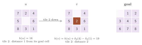
the field of \(b\), two operations on the word (Figure 14.1).
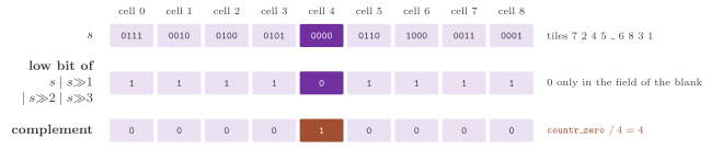
The cell of the blank is not stored: it is found from the word by a few
bitwise operations (Algorithm 14.1, SlidingTile.h:697,
and Figure 14.2), in which \(L = \sum_i 2^{\beta i}\) is the mask
of the lowest bit of each field, \(\gg\) the right shift, \(\mid\), \(\&\) and
\(\sim\) the bitwise or, and and complement, and TZ the number of trailing
zeros of a word.
Algorithm 14.1 (The cell of the blank).
1  procedure BLANK(s)
2     x ← s
3     for k ← 1 to β − 1 do
4        x ← x | (s >> k)       ▷ or the bits of each field into its lowest
5     x ← ~x & L                ▷ one bit set: the lowest of the zero field
6     return TZ(x) / β          ▷ integer division
Lemma 14.1 (The cell of the blank). For every board \(\sigma\) with its blank in the cell \(b\), BLANK\((s)\) returns \(b\), with \(\beta - 1\) shifts and ors and one count of the trailing zeros.
Proof. The bit \(\beta i\) of \(x\) after line 4 is the or of the bits \(\beta i, \beta i + 1, \ldots, \beta i + \beta - 1\) of \(s\), all of which belong to the field of the cell \(i\) (the shifts bring into the higher bits of a field the bits of the next field, but never into its lowest bit, since \(k \le \beta - 1\)). Hence, the bit \(\beta i\) of \(x\) is 0 if and only if the field of \(i\) is 0, i.e., if and only if \(i = b\), the tiles being nonzero and the blank unique. After line 5, \(x = 2^{\beta b}\), and its trailing zeros divided by \(\beta\) give \(b\). \(\square\)
The cells adjacent to each cell are precomputed at construction, in the
order up, left, right and down (SlidingTile.h:255), in a
table \(N(b)\) of at most 25 entries of 5 integers (hence usually in the cache),
and so is the table \(\delta_t(c)\) of the Manhattan distance of the cell \(c\)
from the goal cell of the tile \(t\) (SlidingTile.h:252,
with \(\delta_0 = 0\) for the blank). Also, the domain is an OperatorDomain
whose operator is the cell of the blank in the parent, and Algorithm 14.2 is
its expansion with an operator (SlidingTile.h:341); the
expansion without an operator is the same without line 5
(SlidingTile.h:309).
Algorithm 14.2 (The successors of a board).
1  procedure TILESUCCESSORS(s, h(s), o, f)   ▷ o: the cell the blank left
2     b ← BLANK(s)
3     for each cell c ∈ N(b), in the order up, left, right, down, do
4        if c = o then
5           continue                ▷ the move back to the parent
6        t ← the tile in the field of c of s
7        s' ← s with the field of c set to 0 and that of b set to t
8        f(s', 1, h(s) + δ_t(b) − δ_t(c), b)   ▷ b: the operator of s'
Line 7 is \(s' = (s \mathbin{\&} \sim(m \ll \beta c)) \mid (t \ll \beta b)\), with \(m = 2^\beta - 1\) the mask of a field; since the field of \(b\) is 0 in \(s\), the or writes \(t\) there, and \(s'\) is the packed word of the board with \(t\) and the blank exchanged. Hence an expansion costs one BLANK and, per successor, a constant number of operations on the word and two lookups of \(\delta\), with no loop over the cells; the value of line 8 is the Manhattan distance of \(s'\) by Proposition 14.5 below. The inverse of the move from \(s\) to \(s'\) is the move of the blank of \(s'\) (now in \(c\)) back to \(b\), i.e., to the operator of \(s'\), at the same cost; hence the hypothesis of Lemma 1.8 holds, and line 5 skips only duplicates.
The reachable states¶
Only half of the arrangements of the tiles can be reached from a given
one, and the constructor refuses a start and a goal that are not in the
same half (SlidingTile.h:242), as well as a board that
is not a permutation of \(0, \ldots, WH - 1\). We now state the invariant, after
fixing the notation. For a board \(\sigma\), let \(N(\sigma)\) be the number
of inversions of the tiles read in row-major order without the blank
(the pairs of tiles \(t > t'\) with \(t\) before \(t'\)), and \(r(\sigma)\) the
row of the blank. The function parity
(SlidingTile.h:900) computes \(N(\sigma) \bmod 2\) if \(W\)
is odd and \((N(\sigma) + r(\sigma)) \bmod 2\) if \(W\) is even, by a double loop
over the cells, in \(O((WH)^2)\) time.
Proposition 14.2 (Parity of the sliding-tile puzzles). If \(W\) is odd, \(N(\sigma) \bmod 2\) is invariant under the moves; if \(W\) is even, \((N(\sigma) + r(\sigma)) \bmod 2\) is. Hence, at most half of the \((WH)!\) boards are reachable from a given one.
Proof. A horizontal move does not change the order of the tiles read in row-major order without the blank, nor the row of the blank. A vertical move takes a tile \(t\) over the \(W - 1\) tiles that lie between its cell and that of the blank in row-major order, and changes the row of the blank by 1. Each of these \(W - 1\) tiles forms an inversion with \(t\) before the move but not after it, or conversely, and therefore \(N\) changes by \(W - 1 - 2j\) for some \(j\), i.e., by an even number if \(W\) is odd and by an odd one if \(W\) is even. In the first case \(N \bmod 2\) is preserved; in the second, \(N\) and \(r\) change parity together, and their sum keeps it. Finally, the boards on which the invariant takes the other value are half of the \((WH)!\) boards. In fact, exchanging two tiles changes \(N\) by an odd number and leaves \(r\) unchanged, and it is therefore a bijection between the two halves. \(\square\)
The converse, that every board on which the invariant takes the value of
the start is reachable, is the theorem of Johnson and Story
[150] for the 15-puzzle, and it holds for all
the boards of at least \(2 \times 2\) cells; we use it without
reproducing its proof. Hence, the 8-puzzle has \(9!/2 = 181440\)
reachable states, which the test domains checks by a search of the
whole space, the 15-puzzle \(16!/2 \approx 1.05 \cdot 10^{13}\) and the
24-puzzle \(25!/2 \approx 7.8 \cdot 10^{24}\).
Lemma 14.3 (The blank is uniform). Assume the converse of Proposition 14.2. Then, for each cell \(b\), exactly \((WH - 1)!/2\) reachable boards have the blank in \(b\).
Proof. With the blank fixed in \(b\), the boards are the \((WH - 1)!\) arrangements of the tiles on the other cells, and \(r(\sigma)\) is the same for all of them; hence the invariant is the parity of \(N\), possibly shifted by the constant \(r\). Exchanging two tiles changes the parity of \(N\), and is a bijection between the arrangements of the two parities, which are therefore \((WH - 1)!/2\) each; by the converse, those of the right parity are exactly the reachable ones. \(\square\)
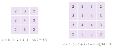
On the puzzles, the branching factor of a state is the number of the neighbours of its blank, 2 in a corner, 3 on a side and 4 inside the board, and by the lemma its mean over the reachable states has a closed form (Figure 14.3).
Proposition 14.4 (Branching factor of the puzzles). Over the reachable states of the puzzle of \(W \times H\) cells, the mean number of moves is \(2(2WH - W - H)/(WH)\), i.e., \(8/3\) for the 8-puzzle, 3 for the 15-puzzle and \(16/5\) for the 24-puzzle; without the move back to the parent it is 1 less on every state but \(s_0\).
Proof. By Lemma 14.3 the blank is uniformly distributed over the cells, and the mean number of moves is the mean degree of a cell in the grid graph of the board, \(2|E|/(WH)\), with \(|E| = H(W - 1) + W(H - 1) = 2WH - W - H\) edges. The three values follow with \(|E| = 12, 24, 40\) (cf. Figure 14.3). Skipping the parent removes exactly one successor of each state but \(s_0\), since the cell left by the blank is adjacent to its current cell. \(\square\)
The Manhattan distance¶
The heuristic is the Manhattan distance: the sum, over the tiles, of the
distance between the cell of the tile and its goal cell in moves of the
grid, \(h(\sigma) = \sum_{t \ne 0} \delta_t(c_\sigma(t))\), with
\(c_\sigma(t)\) the cell of \(t\) in \(\sigma\); computed from scratch, by
heuristic( s ), it takes one lookup per cell.
Proposition 14.5 (The Manhattan distance is consistent). On the sliding-tile puzzle, for each move from \(\sigma\) to \(\sigma'\) of a tile \(t\) from the cell \(c\) to the cell \(b\) of the blank, \(h(\sigma') = h(\sigma) + \delta_t(b) - \delta_t(c)\) and \(|h(\sigma') - h(\sigma)| = 1\); hence, \(h\) is consistent, and therefore admissible.
Proof. Only the tile \(t\) changes its cell, which gives the first identity. The cells \(b\) and \(c\) are adjacent, so that one coordinate changes by 1 and the other not; hence their distances from the goal cell of \(t\) differ by exactly 1, since the distance changes by \(\pm 1\) in that coordinate. Therefore \(h(\sigma) \le 1 + h(\sigma') = c(\sigma, \sigma') + h(\sigma')\), and \(h\) is 0 at the goal; consistency implies admissibility (Lemma 2.4). \(\square\)
The first identity is how Algorithm 14.2 computes \(h\), two lookups instead of a sum over the tiles, which is the incremental heuristic of [4]. The second identity has a consequence on the shape of the search.
Corollary 14.6 (The parity of \(f\)). On the puzzles with the Manhattan distance, \(f = g + h\) changes by 0 or 2 along each edge, and hence the values of \(f\) of all the states generated by a search from \(s_0\) have the parity of \(h(s_0)\).
Proof. Along an edge, \(g\) grows by 1 and \(h\) changes by \(\pm 1\) (Proposition 14.5), so that \(f\) changes by \(0\) or \(2\). A generated state has \(f = g + h\) for the cost \(g\) of a path from \(s_0\), and by induction on the length of the path its parity is that of \(f(s_0) = h(s_0)\). \(\square\)
Hence, iterative deepening raises its bound by exactly 2 at each
iteration on the puzzles, since the least \(f\) above the bound
(Chapter 4) has the parity of the bound.
Of course, the pattern databases of Chapter 5
replace this heuristic in SlidingTilePDB, which keeps the rest of the
domain.
The refinements¶
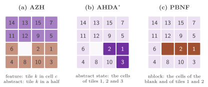
The puzzles model all the refinements of Domain (Figure
14.4). Their feature \(i = tWH + c\) is "tile \(t\) is in cell
\(c\)", for \(t \ne 0\) (num_features() is \((WH)^2\), of which those with
\(t = 0\) are never used). A move changes two features, and
for_each_feature_change (Algorithm 14.3,
SlidingTile.h:420) finds them without knowing the moved
tile, nor the blank.
Algorithm 14.3 (The features changed by a move).
1  procedure FEATURECHANGE(s, s', f)
2     d ← s xor s'                ▷ bitwise exclusive or of the two words
3     if d = 0 then
4        return
5     i ← TZ(d) / β             ▷ the first cell where s and s' differ
6     k ← the field of i of d   ▷ the moved tile
7     j ← TZ(d with the field of i cleared) / β
8     f(k WH + i);  f(k WH + j)
Lemma 14.7 (The features changed by a move).
If \(s'\) is a successor of \(s\), Algorithm 14.3 calls f exactly on the
two features of the symmetric difference of the features of \(s\) and
\(s'\), in constant time.
Proof. Let the move slide the tile \(k\) from \(c\) to the cell \(b\) of the blank of \(s\). The fields of \(s\) and \(s'\) coincide in every other cell; in \(b\) they are \(0\) and \(k\), and in \(c\) they are \(k\) and \(0\). Hence \(d\) has the field \(k \ne 0\) in the two cells \(b\) and \(c\) and 0 elsewhere, line 5 finds the lower of the two, line 6 reads \(k\) in it, and line 7 the higher one. The features that differ are "\(k\) in \(c\)" (in \(s\) only) and "\(k\) in \(b\)" (in \(s'\) only), the blank having no feature, and these are the two calls of line 8. \(\square\)
Next, the abstract feature of AZH (abstract_feature( i )) keeps of
the cell of a tile only whether its row is at least \(\lfloor H/2
\rfloor\) (the lower half of the board) or not, which is the projection
of figure 8(b) of Jinnai and Fukunaga [5] for
the 15-puzzle; there are \(2WH\) abstract features, two per tile.
Proposition 14.8 (The moves that change the abstract features). A horizontal move never changes the abstract features of a board; a vertical move changes them (and then two of them) if and only if it moves a tile between the rows \(\lfloor H/2 \rfloor - 1\) and \(\lfloor H/2 \rfloor\).
Proof. A move changes the cell of one tile only. A horizontal move keeps its row, and hence the half of its cell; a vertical move changes the row by 1, and the half changes if and only if one of the two rows is below \(\lfloor H/2 \rfloor\) and the other is not, i.e., if and only if the rows are \(\lfloor H/2 \rfloor - 1\) and \(\lfloor H/2 \rfloor\); then the abstract feature of the tile in the old half is replaced by that in the new one. \(\square\)
Hence, under HDA\(^*\)[AZ], a successor can have an owner other than that
of its parent only through the moves across the middle of the board (one
pair of rows out of \(H - 1\)), and the others stay on the worker of their
parent; how often such moves occur along a search depends on the
instance and is only measured, not bounded, by the counters of
Chapter 9. As in Burns et al.
[3], the abstract state of AHDA\(^*\)
(abstract_state( s )) is the triple of the cells of tiles 1, 2 and 3,
coded as an integer.
The nblock of PBNF (nblock( s )) is the triple \((p_0, p_1, p_2)\) of the
cells of the blank and of tiles 1 and 2, coded as \((p_0 WH + p_1) WH +
p_2\) among num_nblocks() \(= (WH)^3\) codes, of which only those of three
distinct cells are used. Its abstract successors
(for_each_nblock_successor, SlidingTile.h:548) are the
triples reached by a move of the blank to a cell \(c \in N(p_0)\), which moves
tile 1 or 2 if it lies in \(c\): they are \((c, p_0, p_2)\) if \(c = p_1\), \((c,
p_1, p_0)\) if \(c = p_2\), and \((c, p_1, p_2)\) otherwise. Safe PBNF
requires the two conditions of
Definition 11.1.
Proposition 14.9 (The nblocks of the puzzles).
The nblocks of SlidingTile satisfy Definition
11.1: (i) for each move from \(u\) to \(v\), the
nblock of \(v\) is an abstract successor of that of \(u\), and (ii) the
relation of the abstract successors is symmetric and irreflexive.
Proof. (i) A move takes the blank from \(p_0\) to an adjacent cell \(c\) and the tile of \(c\) to \(p_0\); tile 1 moves if and only if \(c = p_1\), and tile 2 if and only if \(c = p_2\), which are the three cases of the abstract successors. (ii) The blank changes cell in each case, so that no nblock is its own successor. The successor of \((p_0, p_1, p_2)\) through \(c\) has its blank in \(c\), adjacent to \(p_0\), and the move of that blank back to \(p_0\) puts back in \(p_0\) the tile it moved, if any; by the three cases this abstract successor is \((p_0, p_1, p_2)\). \(\square\)
Also, the pairwise heuristic of PA\(^*\)SE (pairwise_heuristic( s , t )) is
the sum over the tiles of the distance between their cells in the two boards,
whose properties are proved with those of the grids and of the vacuum world in
Proposition 14.18. Finally, the perfect hash
(perfect_hash( s )) is the lexicographic rank of the permutation of the
cells of the tiles \(0, 1, \ldots, WH - 1\), i.e., the rank of the pattern
databases of Chapter 5 with all the \(WH\) tiles; by
Lemma 5.4 with \(k = n = WH\), it is a bijection
from the boards onto \([0, (WH)!)\), and it is given only up to 20 cells, since
\(20! < 2^{64} < 21!\). Burns et al. [3] used it as a
work distribution modulo \(p\), and, as Jinnai and Fukunaga
[5] show, modulo \(p\) it then depends on very few
tiles (Proposition 9.14); it is kept as
the poor distribution to compare against.
Instances¶
The file data/15-puzzle/korf100.txt holds the 100 instances of
the 15-puzzle of Korf [7], each with its optimal
cost, which the tests and the benchmarks use as the reference, and
data/24-puzzle/instances50.txt the 50 instances of the
24-puzzle distributed with the code of HDA\(^*\) of Jinnai and Fukunaga. In the
examples, 8Puzzle solves the instance of figure 3.28 of
[13], or the first state found at a given
distance from the goal, and 15Puzzle an instance of Korf, sequentially
or with HDA\(^*\).
14.3 The sequence score of Nilsson¶
SequenceScore< W , H > (SequenceScore.h:54) is the
same puzzle with the heuristic of Nilsson [8],
\(h = M + W S\) (i.e., \(M + 3S\) on the 8-puzzle), where \(M\) is the Manhattan
distance and \(S\) the sequence score. Let \(\mathrm{next}(c)\) be the cell after
\(c\) in the ring, which is, on the \(3 \times 3\) board, the cycle of the
eight cells of the border in clockwise order (the centre having no next
cell), and, on the other boards, the cells \(0, 1, \ldots, WH - 1\) in
row-major order (the last cell having no next cell). The follower
\(\mathrm{fol}(t)\) of a tile \(t\) is the tile that the goal puts in the
next cell of the goal cell of \(t\) or, when that cell has no next cell,
in the cell 0 on the \(3 \times 3\) board and in the cell 1 on the
others. The centre \(c_0\) is the cell 4 on the \(3 \times 3\) board and the
cell 0 on the others. Then
heuristic( s ) is Algorithm 14.4
(SequenceScore.h:110).
Algorithm 14.4 (The sequence score).
1  procedure SEQUENCESCORE(σ)
2     M ← 0;  S ← 0
3     if σ(c₀) ≠ the goal tile of c₀ then
4        S ← 1
5     for each cell c with a tile t = σ(c) ≠ 0 do
6        M ← M + δ_t(c)
7        if next(c) exists and σ(next(c)) ≠ fol(t) then
8           S ← S + 2
9     return M + W · S
It takes \(O(WH)\) time per state, and the successors of SequenceScore
are those of the puzzle with this value computed from scratch for each
of them.
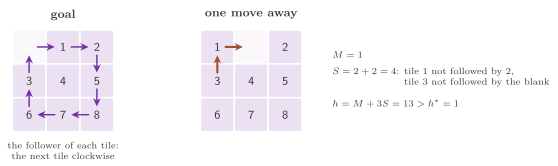
Proposition 14.10 (The sequence score is not admissible). On the 8-puzzle with the goal of Korf, the state one move away from the goal in which tile 1 has moved into the first cell has \(h = 13\), while \(h^* = 1\).
Proof. Only tile 1 is out of place, at distance 1, and \(M = 1\). Since the centre holds tile 4, its goal tile, line 3 adds 0. Along the border (Figure 14.5), tile 1 in the first cell is followed by the blank instead of tile 2, and tile 3 in the cell 3 is followed (in the first cell) by tile 1 instead of the blank, which follows it in the goal; each other tile of the border is followed by its goal follower, and the blank adds nothing (line 5). Hence \(S = 4\) and \(h = 1 + 3 \cdot 4 = 13 > 1\). \(\square\)
Since the heuristic may overestimate, A\(^*\) with it is not guaranteed (cf.
Theorem 2.9) to return an optimal path, and
it does not: on the instance of Figure 14.1 (optimal cost
26, with \(M = 18\) and \(h = 69\)), the example 8Puzzle -h seq returns a
path of 28 moves after fewer than a hundred expansions (a run, not a
bound; the test domains only checks the overestimate of
Proposition 14.10). This domain is there to show this
trade, which weighted A\(^*\) makes with a bound (Chapter
6). It forwards no refinement of
SlidingTile.
14.4 Pathfinding on grids¶
We call grid a rectangular map of \(W \times H\) cells, each "blocked" or free
with a cost \(\kappa(u) \in \{1, \ldots, 255\}\) (GridMap,
Grid.h:82, where cost( x , y ) is 0 for a blocked cell or one
outside the map), on which the agent moves from cell to cell. It is the
benchmark of the video games and of robotics [15],
and many problems reduce to it (the multiple sequence alignment of Chapter
15 is a shortest path on a lattice of higher
dimension). In the library, Grid< Moves > (Grid.h:408) models
pathfinding with 4 moves (up, left, right, down) or 8 (the four diagonals too),
from the cell \((s_x, s_y)\) to the cell \((g_x, g_y)\), and its constructor throws
if either is blocked. A state is the index \(yW + x\) of the cell \((x, y)\), which
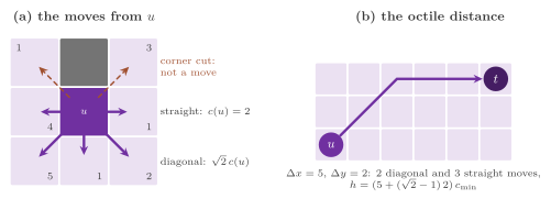
is also the perfect hash. A move leaves a cell at its cost, times \(\sqrt2\)
for a diagonal, i.e., \(c(u, v) = \kappa(u)\) or \(\sqrt2\, \kappa(u)\) (written
cost and sqrt2 in Algorithm 14.5), and a diagonal move is allowed only if both
the cells it cuts are free (Figure 14.6); hence, the costs are
integers with 4 moves and real numbers with 8. The successors are generated by
a GridAdjacency< Moves > (Grid.h:240) with the std and Boost
data structures, and by the grid graph of the default ones, which generates the
same moves at the same costs, in the same order with 4 moves and by increasing
index of the cell with 8 (an order that changes only the ties of OPEN);
Algorithm 14.5 is the former.
Algorithm 14.5 (The moves on a grid).
1  procedure GRIDSUCCESSORS(x, y, f)
2     D ← (0,−1), (−1,0), (1,0), (0,1), (−1,−1), (1,−1), (−1,1), (1,1)
3     for each of the first Moves pairs (δx, δy) of D do
4        (x', y') ← (x + δx, y + δy)
5        if (x', y') is blocked or outside the map then
6           continue
7        if δx ≠ 0 and δy ≠ 0 and ((x', y) or (x, y') is blocked) then
8           continue               ▷ no corner cutting
9        c ← cost(x, y) if δx · δy = 0 else sqrt2 · cost(x, y)
10       f((x', y'), c, h(x', y'))
An expansion thus costs \(O(\mathrm{Moves})\), the heuristic of each successor being a formula of its coordinates (below).
Note that the cost of an edge depends on the cell left: \(c(u, v) =
\kappa(u)\) and \(c(v, u) = \kappa(v)\) differ on a map with several costs.
The graph is therefore directed, and the problem is reversible (in the
sense of §1.2) only on the maps of uniform
cost. A grid is nonetheless an OperatorDomain, since the skip of the
move back to the parent needs only nonnegative costs
(§14.15).
The heuristics¶
The heuristic is the distance on the empty grid times the least cost
\(\kappa_{\min}\) of a free cell (GridMap::min_cost(), 1 if no cell is
free): the Manhattan distance \(d_4(u, t) = \Delta x + \Delta y\) with 4
moves, and the octile distance
with 8 moves, \(\Delta x\) and \(\Delta y\) being the absolute differences of
the coordinates of \(u\) and of the goal \(t\)
(Grid.h:851-854). Our proof of consistency rests on \(d_4\)
and \(d_8\) being the costs of the shortest paths on the grid with no blocked
cell and unit cell costs; for \(d_4\) this is immediate (each move changes
\(\Delta x + \Delta y\) by at most 1, and the straight path attains it), and for
\(d_8\) it is the following lemma.
Lemma 14.11 (The octile distance). On the infinite grid with 8 moves, straight moves of cost 1 and diagonal moves of cost \(\sqrt2\), the least cost of a path between two cells whose coordinates differ by \(\Delta x\) and \(\Delta y\) is \(d_8\).
Proof. A path with \(k\) diagonal and \(l\) straight moves changes the sum of the coordinates by at most \(2k + l\) and each coordinate by at most \(k + l\); hence \(2k + l \ge \Delta x + \Delta y\) and \(k + l \ge \max(\Delta x, \Delta y)\). Its cost is \(\sqrt2\, k + l = (\sqrt2 - 1)(2k + l) + (2 - \sqrt2)(k + l) \ge (\sqrt2 - 1)(\Delta x + \Delta y) + (2 - \sqrt2) \max(\Delta x, \Delta y)\), since both coefficients are positive, and this equals \(d_8\) since \(\Delta x + \Delta y = \max + \min\). The path of \(\min(\Delta x, \Delta y)\) diagonal moves followed by \(|\Delta x - \Delta y|\) straight ones attains the bound. \(\square\)
Proposition 14.12 (The grid heuristics are consistent). On a grid with 4 moves, \(h = \kappa_{\min}\, d_4\) is consistent; on a grid with 8 moves, \(h = \kappa_{\min}\, d_8\) is consistent.
Proof. Both \(d_4\) and \(d_8\) are shortest-path distances on the empty grid (Lemma 14.11 for \(d_8\)), and therefore they satisfy the triangle inequality \(d(u, t) \le d(u, v) + d(v, t)\). For a move from \(u\) to a neighbour \(v\), \(d(u, v)\) is 1 for a straight move and \(\sqrt2\) for a diagonal one, while \(c(u, v)\) is \(\kappa(u) \ge \kappa_{\min}\) times the same factor; hence \(h(u) = \kappa_{\min} d(u, t) \le \kappa_{\min} d(u, v) + \kappa_{\min} d(v, t) \le c(u, v) + h(v)\), and \(h(t) = 0\). Note that the blocked cells and the rule on the corners only remove edges, which keeps the inequality on the remaining ones. \(\square\)
We remark that the Manhattan distance is not admissible with 8 moves,
whether a diagonal move costs \(\sqrt2\) or 1: from \((0, 0)\) to \((1, 1)\)
it gives 2, while one diagonal move costs \(\sqrt2\) (or 1). Also, with 8
moves the costs and the heuristic are computed in double precision, and
Proposition 14.12 holds in exact arithmetic: two paths to
the same cell whose exact costs are equal may differ by an ulp, and a
search may then (rarely) reopen a cell, which costs time but not
optimality (the search of Chapter 2 reopens
whenever it finds a smaller \(g\)). As a check, the test grid compares
A\(^*\) with the algorithm of Dijkstra, written apart from the domain, on
random maps of unit costs and of costs 1 to 5, with 4 and 8 moves, and
the test domains checks the consistency on every edge of three random
maps of costs 1 to 5.
Proposition 14.13 (The moves of an open grid). On a grid of \(W \times H\) free cells, there are \(2(2WH - W - H)\) moves with 4 moves, and \(2(2WH - W - H) + 4(W - 1)(H - 1)\) with 8.
Proof. The straight moves are the two orientations of the \(H(W - 1)\) horizontal and of the \(W(H - 1)\) vertical pairs of adjacent cells. With no blocked cell no diagonal is cut, and each of the \((W - 1)(H - 1)\) squares of \(2 \times 2\) cells has two diagonals, each in two orientations. \(\square\)
On \(5 \times 5\) cells this gives 80 and 144 moves, i.e., the mean
branching factors \(3.2\) and \(5.76\), which the test domains checks.
The refinements and the maps¶
The features of Zobrist hashing are the column and the row of the cell
(\(W + H\) features), the abstract features of AZH the column and the row
of the block of \(B \times B\) cells containing it (\(B\) = block(), 100
by default), and the abstract state of AHDA\(^*\) that block, the two
distributions coinciding on this domain as in section 4.1 of
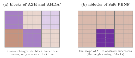
[5]. In turn, the nblocks of PBNF are the
rectangles of GridNBlocks (§14.15), by default the
blocks of \(S \times S\) cells (\(S\) = nblock_side(), 20), and the
abstract successors of an nblock are its 4 (with 4 moves) or 8
(with 8 moves) neighbouring nblocks inside the map (Figure
14.7).
Proposition 14.14 (The nblocks of the
grids). The nblocks of Grid satisfy Definition
11.1.
Proof. (i) A move changes each coordinate by at most 1, and hence the coordinates of the block, \(\lfloor x/S \rfloor\) and \(\lfloor y/S \rfloor\), each by at most 1; with 4 moves only one coordinate changes. Thus the nblock of the successor is that of the parent or one of its neighbours of the right kind, both inside the map. (ii) Being a neighbour is symmetric and irreflexive. \(\square\)
A grid does not model IncrementalFeatureDomain (a move changes one or
two of its features, but the domain does not enumerate them); its
pairwise heuristic for PA\(^*\)SE is
the heuristic between any two cells (Proposition 14.18).
A map is read from a file of the Moving AI benchmarks of Sturtevant
[15] by GridMap::read_movingai (a header
type octile, height, width, map, then the rows, in which ., G and
S are free cells of cost 1 and any other character is blocked). Otherwise,
it is drawn at random by GridMap::random( W , H , p , seed , c_max )
(src/Grid.cpp:53), which blocks each cell with probability \(p\)
and gives each free cell the cost 1 (if \(c_{\max} = 1\)) or a cost drawn
uniformly in \(\{1, \ldots, c_{\max}\}\), row by row. Then it makes the
bottom-left and the bottom-right corners free with cost 1, since they are the
start and the goal of the instances of Burns et al.
[3]. The draws are made from the words of
std::mt19937_64 (Lemma 1.9), and hence a seed
gives the same map on all platforms. In the examples, FindPath finds and
draws a path on such a map.
14.5 Explicit graphs and the map of Romania¶
ExplicitGraph< Cost > (ExplicitGraph.h:144) is a
weighted graph given by its arcs, with nodes \(0, \ldots, n - 1\):
add_edge( u , v , c ) adds an edge (or an arc, with directed), refusing a
negative cost, set_heuristic( u , h ) gives \(h\) node by node (0 by default),
set_source( s ) changes the source, and the search goes from the
source to the target. It serves the small graphs of the tests (e.g., the
graph of Figure 1.3) and the map of
Romania; since \(h\) is given, its admissibility and consistency are the
responsibility of whoever gives it. Its arcs are kept in an
ExplicitAdjacency of the chosen set of data structures
(Chapter 3), which enumerates the arcs that
leave a node in the order of their insertion with the std and the default
sets, but not with that of Boost; the default set also drops a loop \((u,
u)\), which never shortens a path. Its single feature is the node, and
its perfect hash the node itself.
Romania (Romania.h:61) is the road map of figure 3.2 of
Russell and Norvig [13], with 20 cities, 23 roads
whose cost is their length in km, and real costs. Towards Bucharest the
heuristic is the straight-line distance of figure 3.22 of the book;
towards any other city \(t\) it is the Euclidean distance \(e(u, t)\)
between the coordinates of the cities in the code that accompanies the
book (aima-python), both written into the graph by the constructor
(Romania.h:83).
Proposition 14.15 (The heuristics of Romania are consistent). On the map of Romania, the straight-line distance to Bucharest of the book and the Euclidean distance between the coordinates of aima-python, towards any city, are consistent.
Proof. For the Euclidean distance \(e\), the triangle inequality gives
\(e(u, t) \le e(u, v) + e(v, t)\). Also, \(e(u, v)\) is at most the length
of the road \((u, v)\) for each of the 23 roads (the largest ratio of
\(e(u, v)\) to the length of the road is about 0.996, on the road from
Rimnicu Vilcea to Pitesti, on the data of Romania.h); hence
\(h(u) \le c(u, v) + h(v)\), and \(h(t) = 0\). However, the table of the book is
not derived from the coordinates, and its consistency is checked edge by
edge: for each of the 23 roads \((u, v)\), \(|h(u) - h(v)| \le c(u, v)\),
the least slack being 1 km, on the road from Pitesti to Bucharest
(\(100 - 0 \le 101\)), and the next one 4 km, from Rimnicu Vilcea to Pitesti
(\(193 - 100 \le 97\)). Since the roads are two-way, the inequality holds
in both directions. \(\square\)
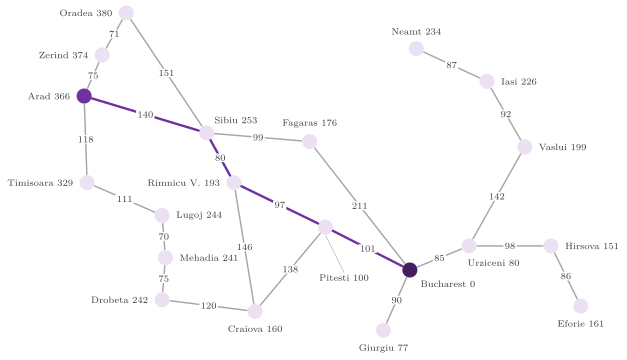
Of course, the proof is a finite check, which the test domains
performs on each edge towards every city, and the test graph checks
what matters to the searches: A\(^*\) finds the 418 km from
Arad to Bucharest of the book, through Sibiu, Rimnicu Vilcea and Pitesti
(Figure 14.8), and the distance to Bucharest from each
city, against a table computed apart. Also, the example RouteFinding
finds a road between any two cities (e.g., RouteFinding Lugoj Neamt).
14.6 Four problems of the textbook¶
The next four domains are problems of chapter 3 of Russell and Norvig [13], each generalized by a size, by which it can be made hard enough to measure a parallel search. They are small in code, and each shows one shape of state space that the searches must handle.
The n-queens problem¶
NQueens (NQueens.h:67) places \(1 \le n \le 32\) queens on an
\(n \times n\) board in the incremental formulation of section 3.2.1 of the
book. A state is the number \(k\) of queens placed and the row \(\mathrm{row}(c)\)
of the queen of each column \(c < k\) (a record of 33 bytes), and a move,
Algorithm 14.6 (NQueens.h:124), adds a queen in the column
\(k\), in a row that no queen already on the board attacks, at cost 1.
Algorithm 14.6 (The successors of a placement).
1  procedure QUEENSUCCESSORS(k, row, h, f)
2     for r ← 0 to n − 1 do
3        if r ≠ row(c) and |r − row(c)| ≠ k − c for each column c < k then
4           f((k + 1, row with row(k) = r), 1, h − 1)
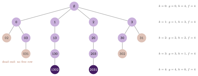
The test of line 3 excludes the rows and the two diagonals of the queens placed; hence an expansion takes \(O(nk)\) time. The state space is a tree whose paths from the root have length at most \(n\), since each state has a single parent (the placement without its last queen), and the goals are the states with \(k = n\); a state of the tree may have no successor, a dead end (Figure 14.9). The features of Zobrist hashing are the pairs (column, row) of the queens placed, and the domain has no perfect hash.
Proposition 14.16 (The heuristic of the queens). The heuristic \(h = n - k\), the number of the empty columns, is consistent, with \(h(u) = c(u, v) + h(v)\) on each edge, and it equals \(h^*\) on the states from which a goal is reachable.
Proof. Each edge adds one queen at cost 1, so that \(h\) drops by exactly 1, and \(h = 0\) at a goal. A state with \(k\) queens from which a goal is reachable needs exactly \(n - k\) more moves to reach it, each move adding one queen. \(\square\)
Hence \(f = n\) on all the states. The ties of \(f\) are broken by the larger
\(g\) (Chapter 3), and A\(^*\) then expands the
states in a depth-first order, backtracking at the dead ends; the
counters of the example NQueens measure how many it meets. The
8-queens problem has 92 solutions, and its tree 2057 states (the root
included), two counts that the test domains obtains by enumerating the
tree; for \(n = 2\) and \(n = 3\) the problem has no solution, and A\(^*\)
reports it after exhausting the tree.
The vacuum world¶
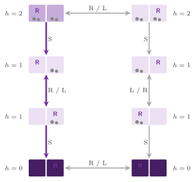
VacuumWorld (VacuumWorld.h:68) is the vacuum world of
section 3.2.1 of the book on a row of \(1 \le n \le 32\) cells instead of 2: a
robot moves Left or Right, or Sucks the dirt of its cell, each action
costing 1, and the goal is a clean row. A state packs the set \(D\) of the
dirty cells in the bits 0 to 31 of a word and the cell \(r\) of the robot
in the bits 32 to 37, and the word is also the perfect hash; Algorithm
14.7 is its expansion (VacuumWorld.h:128).
Algorithm 14.7 (The successors in the vacuum world).
1  procedure VACUUMSUCCESSORS(r, D, h, f)
2     if r ∈ D then
3        f((r, D ∖ {r}), 1, h − 1)      ▷ Suck
4     if r > 0 then
5        f((r − 1, D), 1, h)            ▷ Left
6     if r + 1 < n then
7        f((r + 1, D), 1, h)            ▷ Right
Proposition 14.17 (The vacuum world). From a start with all the cells dirty, all the \(n 2^n\) states are reachable; the heuristic \(h = |D|\) is consistent; and the nblocks of PBNF, i.e., the cells of the robot with the neighbouring cells as abstract successors, satisfy Definition 11.1.
Proof. A state \((r, D)\) is reached from \((r_0, \{0, \ldots, n-1\})\) by
walking along the row and sucking every cell not in \(D\), and then by
walking to \(r\). A Suck lowers \(h\) by 1 at cost 1 and a move leaves it
unchanged, so that \(h(u) \le c(u, v) + h(v)\) on each edge, and \(h = 0\)
at a goal. Finally, an action keeps the cell of the robot or moves it to
a neighbour, and being neighbours is symmetric and irreflexive. \(\square\)
The heuristic is also "weak", since it ignores the moves needed to reach
the dirt, which usually cost about as much as the cleaning. Furthermore,
the domain models the other abstractions of the parallel searches, all
of which keep the dirt and forget the robot. Thus, the features of
Zobrist hashing are the dirty cells \(i < n\) and the cell \(n + r\) of the
robot, the abstract features of AZH are the dirty cells (the \(n\)
features of the robot being mapped to one abstract feature, which all the
states have), and the abstract state of AHDA\(^*\) is \(D\); hence, a move
keeps the owner of a state under these two distributions, and only a
Suck may change it.
The pairwise heuristic of PA\(^*\)SE between \(s\) and \(t\),
pairwise_heuristic( s , t ), is the number of the cells dirty in \(s\)
and clean in \(t\). We now prove the properties (H1) and (H3) that PA\(^*\)SE
requires (stated in Chapter 8, where
PA\(^*\)SE is given) for the pairwise heuristics
of the three domains that have one, \(h(t, s)\) being the pairwise
heuristic and \(d(t, s)\) the least cost of a path from \(t\) to \(s\).
Proposition 14.18 (The pairwise heuristics). For the sliding-tile puzzles with the Manhattan distance, the grids with \(\kappa_{\min} d_4\) or \(\kappa_{\min} d_8\) and the vacuum world with \(|D|\), the pairwise heuristic satisfies (H1) \(h(t, s) \le d(t, s)\) and (H3) \(h(t) \le h(t, s) + h(s)\), for all states \(t\) and \(s\).
Proof. On the puzzles, \(h(t, s) = \sum_{k \ne 0} \mathrm{dist}(c_t(k),
c_s(k))\), with dist the Manhattan distance between cells; a move changes
the cell of one tile by one step, and hence \(h(t, \cdot)\) by at most 1,
which gives (H1), and the triangle inequality of dist, tile by tile,
gives (H3), since \(h(t)\) is the same sum with the goal in place of \(s\).
On the grids, \(h(t, s) = \kappa_{\min} d(t, s)\) for \(d = d_4\) or \(d_8\):
(H1) is the argument of Proposition 14.12 with \(s\) in
place of the goal, and (H3) is the triangle inequality of \(d\). On the
vacuum world, \(h(t, s) = |D_t \setminus D_s|\): each cell of \(D_t
\setminus D_s\) needs a Suck on any path from \(t\) to \(s\), which gives
(H1), and \(|D_t| \le |D_t \setminus D_s| + |D_s|\), which is (H3).
\(\square\)
The water jugs¶
WaterJugs (WaterJugs.h:67) is the problem of exercise
3.6(d) of the book (the PourProblem of aima-python). Up to 4 jugs of
capacities \(\gamma_j \le 65535\) units are empty at the start, a move fills a
jug from the faucet, empties it on the ground, or pours it into another jug
until either the first is empty or the second is full, and the goal is a
jug holding a given quantity \(q\) (Figure 14.11). Every move
costs 1, and the moves that do not change the state are not generated
(Algorithm 14.8, WaterJugs.h:133, where \(L\) is the vector
of the levels). In the state, the level \(L_j\) of the jug \(j\) is packed in the
bits \(16j\) to \(16j + 15\), and the word is also the perfect hash; the
features of Zobrist hashing are the pairs
(jug, level).
Algorithm 14.8 (The successors of the water jugs).
1  procedure JUGSUCCESSORS(L, f)
2     for each jug i do
3        MOVE(L with Lᵢ = γᵢ)                     ▷ fill i
4        MOVE(L with Lᵢ = 0)                      ▷ empty i
5        for each jug j ≠ i do
6           δ ← min(Lᵢ, γⱼ − Lⱼ)
7           MOVE(L with Lᵢ = Lᵢ − δ and Lⱼ = Lⱼ + δ)   ▷ pour i into j
8  procedure MOVE(L')
9     if L' ≠ L then
10       f(L', 1, h(L'))
An expansion generates at most \(J^2 + J\) states with \(J\) jugs, each with the goal test of \(O(J)\) that gives its heuristic, in \(O(J^3)\) time.
Proposition 14.19 (The water jugs). The heuristic, 0 at a goal and 1 elsewhere, is consistent. A goal is reachable only if \(q\) is a multiple of the greatest common divisor \(\gamma\) of the capacities and \(q \le \max_j \gamma_j\).
Proof. Along an edge of cost 1 the heuristic changes by at most 1, and it is 0 at the goals. For the second claim, each level is a multiple of \(\gamma\) at the start, and lines 3, 4 and 7 keep it so: \(\gamma_i\), 0, and \(\delta\), the minimum of two multiples of \(\gamma\), are multiples of \(\gamma\); also, no level exceeds the capacity of its jug. \(\square\)
The heuristic is (perhaps) the best estimate that does not use the number theory of the capacities; the converse of the condition is not needed by the domain, which leaves an instance that violates it to be proved unsolvable by the search. Note that the problem is not reversible: emptying a jug cannot be undone in one move.

The missionaries and cannibals¶
MissionariesCannibals
(MissionariesCannibals.h:65) is the problem of
exercise 3.9 of the book with \(m \le 65535\) missionaries, \(c \le 65535\)
cannibals and a boat of \(b \ge 1\) seats: everybody starts on the left bank with
the boat, a crossing carries from 1 to \(b\) people, and on neither bank may the
missionaries be outnumbered by the cannibals if any missionary is there. Every
crossing costs 1. A state packs the numbers \(m_L\) and \(c_L\) of the missionaries
and the cannibals on the left bank and the bank of the boat, and the word is
the perfect hash; the features of Zobrist hashing are \(m_L\), \(c_L\) and the
bank. Algorithm 14.9 is the expansion
(MissionariesCannibals.h:146), where
\((a_m, a_c)\) are the people on the bank of the boat and safe\((x, y)\) means
\(x = 0\) or \(x \ge y\).
Algorithm 14.9 (The crossings).
1  procedure CROSSINGS(m_L, c_L, boat, f)
2     (a_m, a_c) ← the people on the bank of the boat
3     for d_m ← 0 to min(a_m, b) do
4        for d_c ← (0 if d_m > 0 else 1) to min(a_c, b − d_m) do
5           (m', c') ← the people left on the left bank after the crossing
6           if safe(m', c') and safe(m − m', c − c') then
7              f((m', c', the other bank), 1, h(m', c', the other bank))
The heuristic counts the crossings that would carry the \(n = m_L + c_L\)
people left on the left bank over the river with the boat always full,
heuristic( s )
(MissionariesCannibals.h:129):
with \(h = h_L(n)\) if the boat is on the left bank and \(h = h_L(n) + 1\) otherwise (for \(n > 0\)).
Proposition 14.20 (Admissible, not
consistent). The heuristic of MissionariesCannibals is admissible. It
is not consistent: with 3 missionaries, 3 cannibals and a boat of 2
seats, the first crossing of an optimal solution lowers it by 3.
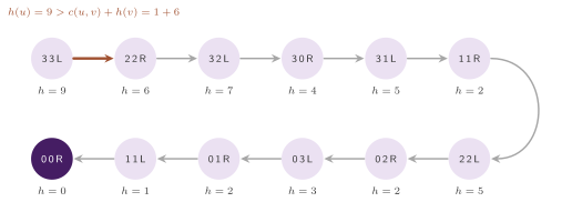
Proof. With the boat on the left, a solution alternates crossings to the right, each carrying at most \(b\) people, and crossings back, each bringing at least 1. After \(k\) round trips at most \(k(b - 1)\) people have left, and the last crossing carries at most \(b\); hence \(n \le k(b - 1) + b\), i.e., \(k \ge \lceil (n - b)/(b - 1) \rceil\) for \(n > b\) and \(b > 1\), and the solution has at least \(2k + 1\) crossings; for \(0 < n \le b\) it has at least 1. For \(b = 1\) no round trip makes progress, no solution exists when \(n > 1\), and \(h^* = +\infty\) bounds any value. With the boat on the right and \(n > 0\), the first crossing brings back \(j \ge 1\) people, and the rest needs at least \(h_L(n + j) \ge h_L(n)\) crossings, \(h_L\) being nondecreasing; hence \(h^* \ge 1 + h_L(n)\), the value of \(h\). For the second claim, the start has \(n = 6\) and \(h = 2 \lceil 4/1 \rceil + 1 = 9\); carrying a missionary and a cannibal (the first crossing of the solution of Figure 14.12) leaves \(n = 4\) with the boat on the right, \(h = 2 \lceil 2/1 \rceil + 1 + 1 = 6\), and \(9 > 1 + 6\). \(\square\)
The proof shows where the slack may be: on the right bank the heuristic
adds 1 to \(h_L(n)\), while the argument gives \(1 + h_L(n + 1)\), which is
larger by 2 for some \(n \ge b\) (for each \(n \ge b\) when \(b = 2\)). With
3, 3 and 2 the answer is 11 crossings, and with 4, 4 and 2 there is no
solution, as the test domains checks by exhausting the state space.
A\(^*\) is optimal with an admissible heuristic, reopening the closed
states when needed (Theorem 2.9); the
searches that assume consistency are not. For instance, the search with
delayed duplicate detection of Chapter 4
refuses a successor of a smaller \(f\) than its parent with an exception
(DDDAStar.h:363), and it does so on this domain.
14.7 The traveling salesperson problem¶
TravelingSalesman (TravelingSalesman.h:78) finds
a tour of least cost through \(2 \le n \le 32\) cities, starting and ending at
the city 0, given the matrix \(d\) of the distances (random_cities( n , seed )
draws \(n\) points of the unit square and gives their Euclidean distances). A
state is the set \(S\) of the visited cities and the current one \(c\),
packed as \(S\) in the bits 0 to 31, \(c\) in the bits 32 to 36 and, in the
bit 37, whether the tour has gone back to the city 0; the word is also
the perfect hash, and the features of Zobrist hashing are the visited
cities, the current one and the closing of the tour. The start is \(S =
\{0\}\), \(c = 0\), and Algorithm 14.10 is the expansion
(TravelingSalesman.h:227).
Algorithm 14.10 (The successors of a partial tour).
1  procedure TOURSUCCESSORS(S, c, f)
2     if S = {0, …, n − 1} then
3        f(the closed tour, d(c, 0), 0)     ▷ the goal
4        return
5     for each city k ∉ S, by increasing k, do
6        f((S ∪ {k}, k), d(c, k), MST((V ∖ (S ∪ {k})) ∪ {k, 0}))
The heuristic of a state \(u\) with current city \(c\) and set \(U = V
\setminus S\) of unvisited cities (\(V\) being the set of all the cities)
is the cost \(\mathrm{MST}(U \cup \{c, 0\})\) of a minimum spanning tree of
the unvisited cities together with the current and the first one
(exercise 3.30 of [13]), and 0 at the goal;
it is computed by the algorithm of Prim on the complete graph of these
\(m\) cities, Algorithm 14.11
(TravelingSalesman.h:190), in \(O(m^2)\) time.
Algorithm 14.11 (The algorithm of Prim).
1  procedure MST(u₁, …, u_m)
2     key(u₁) ← 0;  key(u_k) ← ∞ for k > 1;  T ← ∅;  w ← 0
3     for it ← 1 to m do
4        x ← the city not in T of least key
5        T ← T ∪ {x};  w ← w + key(x)
6        for each city y ∉ T do
7           key(y) ← min(key(y), d(x, y))
8     return w
Lemma 14.21 (The algorithm of Prim). If \(d\) is symmetric, Algorithm 14.11 returns the cost of a minimum spanning tree of the complete graph on \(u_1, \ldots, u_m\) with the costs \(d\).
Proof. Let the city \(x\) of line 4 be joined to the city of \(T\) for which its key was last lowered at line 7 (none for \(u_1\)); then \(w\) is the cost of the tree \(F\) so built on \(T\), since key\((x)\) is the least cost of an edge from \(x\) to \(T\). We show by induction on \(|T|\) that \(F\) is contained in a minimum spanning tree. Let \(F^*\) be a minimum spanning tree containing \(F\) before \(x\) joins, and let \(e = (x, y)\), \(y \in T\), be the edge added. If \(e \notin F^*\), the path of \(F^*\) from \(x\) to \(y\) crosses the cut between \(T\) and the rest by an edge \(e'\), of cost at least key\((x)\), since \(x\) has the least key among the cities outside \(T\) and the key of a city is its least edge to \(T\); replacing \(e'\) by \(e\) gives a spanning tree of cost at most that of \(F^*\), which contains \(F \cup \{e\}\). After \(m\) steps \(F\) spans all the cities, and it is a minimum spanning tree. \(\square\)
Its state space is small, as an exhaustive count shows.
Proposition 14.22 (The states of the tour). The states reachable from the start are \((n - 1)\, 2^{n-2} + 2\): the start, the closed tour, and the pairs of a nonempty set \(S' \subseteq \{1, \ldots, n - 1\}\) and of a current city \(c \in S'\), the visited set being \(S' \cup \{0\}\).
Proof. Line 6 adds to \(S\) the city it moves to, so that every state but the start and the closed tour has its current city in \(S \setminus \{0\}\); conversely, each pair \((S', c)\) is reached by visiting the cities of \(S' \setminus \{c\}\) in any order and then \(c\). There are \(\sum_{j=1}^{n-1} \binom{n-1}{j} j = (n - 1)\, 2^{n-2}\) such pairs. \(\square\)
One can compare this number with the \((n - 1)!/2\) tours of a symmetric instance: this is the state space of the dynamic program of Held and Karp [14], and A\(^*\) on it explores a part of that table, the part selected by the heuristic.
Proposition 14.23 (The MST heuristic is
consistent). If the distances are symmetric and nonnegative, the
heuristic of TravelingSalesman is consistent, and hence admissible.
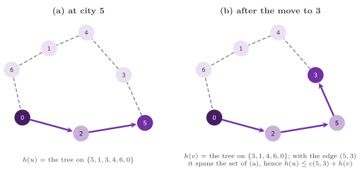
Proof. Let \(u\) have current city \(c\) and unvisited set \(U \ne \emptyset\), and let \(v\) be the successor that moves to \(k \in U\); thus, \(v\) has current city \(k\) and unvisited set \(U \setminus \{k\}\), and \(h(v) = \mathrm{MST}(U \cup \{0\})\). A minimum spanning tree of \(U \cup \{0\}\) together with the edge \((c, k)\) is a spanning tree of \(U \cup \{c, 0\}\), of cost \(h(v) + d(c, k)\) (if \(c = 0\) the edge is not needed); hence \(h(u) \le d(c, k) + h(v) = c(u, v) + h(v)\) (Figure 14.13). When \(U = \emptyset\) and \(c \ne 0\), the only successor is the goal, at cost \(d(c, 0)\), and \(h(u) = \mathrm{MST}(\{c, 0\}) = d(c, 0) = c(u, v) + 0\); at the goal \(h = 0\). The values of \(h\) are those of a minimum spanning tree by Lemma 14.21. \(\square\)
We remark that the proof needs the symmetry, since a spanning tree is a
set of undirected edges; on an asymmetric matrix Algorithm 14.11 still
returns a number (it reads \(d\) from the tree towards the other cities),
but the proposition no longer applies. Admissibility is also seen
directly: the rest of a tour from \(u\) is a path from \(c\) through all the
cities of \(U\) to 0, i.e., a spanning tree of \(U \cup \{c, 0\}\), and it
costs at least the minimum one. An expansion costs \(O(n^3)\), i.e., one
MST of \(O(n^2)\) for each of the at most \(n - 1\) successors; the test
domains checks the consistency on every edge of the state spaces of 5
to 9 random cities, and the number of states of
Proposition 14.22.
The header also gives the dynamic program of Held and Karp
[14], as held_karp()
(TravelingSalesman.h:300), by which the test
domains and the example TravelingSalesman check the cost found by A\(^*\)
(the example up to 20 cities). With \(C(S, j)\) the least cost of a path that
starts at the city 0, visits exactly the cities of the set \(S \ni 0\) and ends
at \(j \in S\), it rests on the recurrence
\(C(S \cup \{k\}, k) = \min_{j \in S} \{C(S, j) + d(j, k)\}\) for \(k \notin S\),
and the optimal tour costs \(\min_{j \ne 0} \{C(V, j) + d(j, 0)\}\).
Algorithm 14.12 (The dynamic program of Held and Karp).
1  procedure HELDKARP(d, n)
2     C({0}, 0) ← 0;  C(S, j) ← ∞ for each other pair
3     for each set S ∋ 0, by increasing value of its bits, do
4        for each j ∈ S with C(S, j) < ∞ do
5           for each k ∉ S do
6              C(S ∪ {k}, k) ← min(C(S ∪ {k}, k), C(S, j) + d(j, k))
7     return min over j ≠ 0 of C(V, j) + d(j, 0)
Proposition 14.24 (Held and Karp). Algorithm 14.12 returns the cost of an optimal tour, in \(O(2^n n^2)\) time with a table of \(2^n n\) entries.
Proof. The recurrence holds since the last edge of an optimal path that ends at \(k\) is some \((j, k)\), and the rest is a path that visits \(S\) and ends at \(j\), which may be replaced by an optimal one. Line 3 visits each set after all its subsets, since adding a city raises the value of the bits; hence, when \(S\) is visited, every \(C(S, j)\) has received at line 6 all the terms of its recurrence, and by induction on \(|S|\) it is final. A tour is a path through \(V\) ending at some \(j \ne 0\), followed by \((j, 0)\), which gives line 7. The table has \(2^n\) sets times \(n\) cities, and lines 4 to 6 take \(O(n^2)\) per set. \(\square\)
The time and the memory are why the method serves to check the searches on small instances only.
14.8 Slow expansions¶
SlowDomain< D > (SlowDomain.h:60) wraps a domain D and
adds to each expansion (both for_each_successor, the one with an operator
included) a given number \(w\) of iterations of the computation \(i
\leftarrow 11 i \bmod 9999943\), from \(i = 7\)
(SlowDomain.h:151), which keeps a core busy with no
access to memory, as in the experiment of section 3.1.1 of Jinnai and Fukunaga
[5] on the effect of slow expansions. It models the
problems in which the expansion dominates the cost of a search (planning with
an expensive heuristic, or motion planning with collision checks), the regime
in which PA\(^*\)SE of Chapter 8 is meant to pay.
The result of the loop is added to a thread-local variable, which is
visible outside the function, and therefore the compiler may not remove
the loop.
Proposition 14.25 (A slow domain is the same
problem). SlowDomain< D > has the states, the initial state, the
goals, the edges with their costs, the heuristic, the hash and the
refinements of D but IncrementalFeatureDomain; hence every guarantee
of a search on D holds on it, and each expansion costs \(\Theta(w)\)
more.
Proof. Each method of the wrapper calls the method of the same name of
D with the same arguments, the expansions after the busy loop, which
changes no state of the search. \(\square\)
Since IncrementalFeatureDomain is not forwarded, the Zobrist keys of
the successors of a slow domain are computed from scratch; with an
expansion that is slow by construction, this cost is negligible. In the
benchmark, the option --slow gives \(w\).
14.9 The pancake problems¶
PancakePuzzle< N > (Pancake.h, \(2 \le N \le 254\)) is the
pancake problem of Dweighter [63]: a stack of \(N\)
pancakes of the sizes \(0, \ldots, N - 1\) is an array of \(N\) bytes, the
size of each pancake from the top, and the flip of \(k\), \(2 \le k \le N\),
reverses the top \(k\) pancakes at cost 1; the goal is the identity, the
largest pancake at the bottom. Its constructor takes the start and the
\(x\) of the heuristic GAP-\(x\) (0 for the gap heuristic), and refuses a
start that is not a permutation; the heuristic and its properties are
those of §5.16 (Proposition
5.21), and the successors receive it
incrementally, by the change of the one pair at the boundary of the
flip (Figure 14.14). The successors are generated from
the flip of \(N\) down to the flip of 2 (Algorithm 14.13, which transcribes the code; the header has no
pseudocode), the operator of the flip of \(k\) is \(k\), and since a flip is
its own inverse, at the same cost, the expansion with an operator skips
it, which Lemma 1.8 justifies.
Algorithm 14.13 (The flips of a stack).
1  procedure FLIPS(p, h, o, f)    ▷ o: the flip that made p (none at the root)
2     for k ← N down to 2 do
3        if k = o then continue
4        b ← p[k] if k < N else the plate
5        h' ← h − gap(p[k − 1], b) + gap(p[0], b)
6        f(p with p[0..k−1] reversed, 1, h', k)
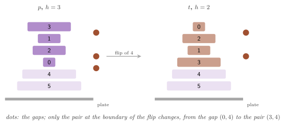
The features of Zobrist hashing are the \(N^2\) pairs (position, size),
and the features changed by a flip of \(k\) are found by comparing the two
stacks position by position, i.e., in \(O(N)\) time; the perfect hash is
the lexicographic rank of the stack, by LexRanking of
§5.14, for \(N \le 20\). The domain is also
a PermutationDomain of one group of \(N\) positions without orientations,
whose moves are the flips, so that the tables of
§5.15 apply to it. A stack is read from a
text by parse( text ), its sizes from the top separated by blanks, and
random( seed ) draws a uniformly random stack, the same for a seed on
every platform, by the shuffle of Fisher and Yates on the words of
std::mt19937_64 (Lemma 1.9).
In BurnedPancakePuzzle< N > (\(1 \le N \le 127\)) each pancake also has a
side burned: a pancake is a byte, its size in the low 7 bits and the bit
7 (turned) set if the burned side is up, a flip of \(k\), now for \(1 \le
k \le N\), also turns every pancake it moves (the flip of 1 only turns
the top pancake), and the goal is the identity with no pancake turned.
The heuristic counts the pairs that are not good (Proposition
5.22), incrementally as above; the features
are the \(2N^2\) triples (position, size, side), there is no perfect hash,
and the domain is a PermutationDomain of one group of modulus 2, the
flip of \(k\) turning the positions \(0, \ldots, k - 1\). In a text, a
pancake is its size plus one, negative if it is turned (e.g., -3 1 -2 5
4), and random( seed ) also turns each pancake with probability
\(1/2\).
Proposition 14.26 (The stacks are connected). Every stack of \(N \ge 2\) pancakes reaches the goal in at most \(2N - 3\) flips, and every stack of \(N\) burned pancakes in at most \(3N\); since the flips are involutions, the \(N!\) stacks, and the \(N!\, 2^N\) burned ones, are all reachable from any of them.
Proof. For \(j = N - 1\) down to 2, if the pancake \(j\) is not at the position \(j\), one flip brings it to the top (none if it is there), and the flip of \(j + 1\) puts it at the position \(j\), leaving the positions below untouched; the two pancakes left are then sorted by at most one flip of 2, which gives \(2(N - 2) + 1\) flips. With the burned pancakes, for \(j = N - 1\) down to 0, one flip brings the pancake \(j\) to the top, the flip of 1 turns it if it is not turned, and the flip of \(j + 1\) puts it at the position \(j\) with its burned side down, i.e., at most 3 flips for each pancake. A flip being its own inverse, the graph is undirected, and a stack is reachable from another through the goal. \(\square\)
The bounds are those of the method of the proof, not the diameters of
the graphs, which are much harder questions. The test pancake checks
the \(7! = 5040\) stacks of 7 pancakes and the \(5!\, 2^5 = 3840\) stacks of
5 burned pancakes, all reached from the goal, and the reading of a
burned stack. In the benchmark, AStarBench --domain pancake takes \(N\)
from --size (12, 16, 20, 32 or 64) and the \(x\) of GAP-\(x\) from
--gap, --domain burned takes \(N\) = 8, 10, 12 or 16, a random stack
for each seed of --ids, and --pdb k adds the tables of the first \(k\)
objects, of the next \(k\), and so on.
14.10 TopSpin¶
TopSpin< N , K > (TopSpin.h, \(2 \le K \le N < 255\), \(K = 4\) by
default) is the TopSpin puzzle of Felner et al.
[167]: \(N\) tokens on a ring, and a turnstile
that reverses \(K\) consecutive tokens. A state is an array of \(N\) bytes,
the token at each position; the move \(i\), \(0 \le i < N\), reverses the
tokens at the positions \(i, \ldots, i + K - 1\) modulo \(N\) at cost 1, and
the goals are the \(N\) rotations of the identity, i.e., the tokens in
increasing order around the ring wherever the token 0 is. The
constructor refuses a start that is not a permutation; the heuristic,
\(\lceil b / 2 \rceil\) for \(b\) breakpoints, is that of Proposition
5.23, computed anew for each successor in
\(O(N)\) time. The operator of the move \(i\) is \(i\), its own inverse, which
the expansion with an operator skips; for the tree searches, the domain
is also a TreeOperatorDomain (Domain.h), whose
for_each_tree_successor skips, after the move \(i\), the moves \(j < i\)
whose turnstiles are disjoint from that of \(i\), since two such moves
commute. The test of disjointness is commute( i , j ): with \(d = (j -
i) \bmod N\), the turnstiles are disjoint if and only if \(d \ge K\) and \(N -
d \ge K\). The features are the pairs (position, token), the perfect hash
the lexicographic rank of the ring for \(N \le 20\), and the domain is a
PermutationDomain of one group whose goals are the \(N\) rotations;
parse( text ) reads a ring from the position 0, and random( seed , n
) is a uniform ring if \(n = 0\) and the identity after \(n\) random moves
otherwise. The pruning of the tree searches is an instance of a general
rule, which serves also Rubik's cube and the Towers of Hanoi.
Lemma 14.27 (Redundant pairs of moves). Let a
TreeOperatorDomain skip, after a move \(a\), (i) moves \(b\) such that \(a\)
followed by \(b\) has the effect of a single move \(m\), or of none, at a
cost not larger than \(c(a) + c(b)\), and (ii) moves \(b \prec a\) that
commute with \(a\), for a strict order \(\prec\) of the moves fixed in
advance. Then for every
path from \(s\) to \(t\) there is a path from \(s\) to \(t\), of a cost not
larger, whose consecutive pairs of moves are never skipped; hence IDA\(^*\)
and the parallel IDA\(^*\), which enumerate the kept paths only, remain
complete and optimal.
Proof. Rewrite the path as long as it has a skipped pair: a pair of type (i) is replaced by the single move \(m\) or removed, which shortens the path and does not raise its cost, and a pair of type (ii), \(a\) followed by \(b \prec a\), is replaced by \(b\) followed by \(a\), which reaches the same state at the same cost, has the same length and one inverted pair fewer under \(\prec\) (the number of the pairs of positions \(p < q\) whose moves satisfy \(m_q \prec m_p\) decreases by exactly one by an exchange of adjacent moves). The pair (length, number of inverted pairs) decreases in the lexicographic order at each step, and the rewriting ends with a path that has no skipped pair, from \(s\) to \(t\) and of a cost not larger than the original one. The searches of the lemma try every kept move at each node, so that they enumerate every path without skipped pairs, among which a cheapest path to a goal. \(\square\)
For TopSpin, (i) is the repetition of a move, whose effect is none, and
(ii) the disjoint turnstiles with the order of their indices. We remark
that the searches with a closed list do not use these prunings
(Domain.h, the comment of the concept), since the kept path to a
state may go through a state closed with another operator; they use only the
skip of the inverse, by Lemma 1.8. The test
topspin checks, on the \(8! = 40320\) rings of TopSpin with 8 tokens and
a turnstile of 4, all reachable from the goals, the consistency of the
breakpoints and of a table of 5 tokens, and IDA\(^*\) and A\(^*\) with and
without the table against the exact distances. In the benchmark,
AStarBench --domain topspin takes \(N\) = 12, 14, 16 or 17 with \(K = 4\),
the identity after 1000 random moves for each seed.
14.11 Rubik's cube¶
RubiksCube (RubiksCube.h) is Rubik's cube in the half-turn
metric, in the cubie model of Kociemba [172]:
a state is the cubie and the
orientation at each of the 8 corner and 12 edge positions, in the order
of Kociemba (the corners URF, UFL, ULB, UBR, DFR, DLF, DBL, DRB and the
edges UR, UF, UL, UB, DR, DF, DL, DB, FR, FL, BL, BR), stored as an array
of 20 bytes that holds \(3c + o\) at the corner positions 0 to 7 and \(2e +
o\) at the edge positions 8 to 19, \(c\) and \(e\) being the cubies and \(o\)
their orientations. A move turns a face (U, R, F, D, L or B) by a
quarter turn clockwise, a half turn or a quarter turn counterclockwise,
at cost 1, and its operator is \(3f + t\) for the face \(f\) and the turn
\(t \in \{0, 1, 2\}\). The 18 moves are tables of 20 positions, the
permutation \(\mathrm{from}\) and the turns: the cubie that comes to the
position \(i\) is the one at \(\mathrm{from}[i]\), its orientation grown by
\(\mathrm{turn}[i]\) modulo 3 (corners) or 2 (edges). They are built once
from the six quarter turns of the cubie model by composition (the move
\(a\) followed by \(b\) has \(\mathrm{from}[i] = \mathrm{from}_a[\mathrm{from}_b[i]]\)
and \(\mathrm{turn}[i] = \mathrm{turn}_a[\mathrm{from}_b[i]] +
\mathrm{turn}_b[i]\)), so that the cube is a PermutationDomain of two
groups, the corners and the edges, whose orientations sum to 0. The
heuristic of the domain is 0, the tables of Korf being given by
RubikPDBHeuristic and PDBDomain of
§5.16. The features of Zobrist hashing are
the \(20 \cdot 24\) pairs (position, value), with their changes, and the
domain has no perfect hash. parse_moves( text ) reads a sequence of
moves in the notation of Singmaster (a face, followed by nothing, by 2,
or by - or '), scramble( text ) applies it to the solved cube
(solved()), and random_walk( n , seed ) makes \(n\) random moves, each
of a face other than the last one.
The expansion with an operator skips the three turns of the face just
turned. for_each_tree_successor also skips the turns of the face
opposite to the one just turned when that face comes second in its pair
of opposite faces in the order U, R, F, D, L, B (after D it skips U,
after L it skips R, and after B it skips F), since two turns of opposite
faces commute. These are the prunings of Korf
[59], to which Lemma 14.27 applies: two turns
of one face make a single turn of that face or none, and the faces are
ordered as above.
Proposition 14.28 (The moves of the cube). (i) Each move has order 4 (a quarter turn) or 2 (a half turn), and the inverse of the move \(3f + t\) is \(3f + 2 - t\). (ii) The skip of the three turns of the face just turned changes neither the outcome nor the order of the expansions of a search that keeps CLOSED, never increases a \(g\) and keeps the expanded states. (iii) With the prunings of the tree searches, the number of the nodes at the depth \(d \ge 1\) of the tree is \(x_d + y_d\), with \(x_1 = y_1 = 9\), \(x_{d+1} = 6 x_d + 6 y_d\) and \(y_{d+1} = 9 x_d + 6 y_d\), i.e., 18, 243, 3240, 43254 and 577368 nodes at the depths 1 to 5, and its asymptotic branching factor is \(6 + 3 \sqrt{6} \approx 13.34847\).
Proof. (i) The tables of the turns \(t = 0, 1, 2\) of a face are the first three powers of its quarter turn, which has order 4 in the cubie model; hence the turn \(t\) followed by the turn \(2 - t\) is the fourth power, the identity. (ii) Let \(u\) be generated from \(v\) by a turn of the face \(f\); a second turn of \(f\) from \(u\) leads to \(v\) itself, or to a state \(w\) that is a single turn of \(f\) away from \(v\), i.e., a sibling of \(u\). In the first case Lemma 1.8 applies. In the second, \(w\) is generated by the expansion of \(v\), which precedes that of \(u\), with the cost \(g(v) + 1\), and the cost of \(w\) known when \(u\) is expanded is at most that value, since a \(g\) never increases, while the skipped generation would give \(g(u) + 1 \ge g(v) + 2\); the generation would thus be a duplicate, which changes nothing but the counters. (iii) Let \(x_d\) and \(y_d\) count the nodes at the depth \(d\) whose last face is the first of its pair (U, R, F) and the second (D, L, B). At the depth 1 there are 9 of each. After a first face, the 5 other faces are kept, 2 first and 3 second ones, with 3 turns each; after a second face, the 4 faces other than it and its opposite are kept, 2 of each kind; this gives the recurrence and the counts. The matrix \(\begin{pmatrix} 6 & 6 \\ 9 & 6 \end{pmatrix}\) has the eigenvalues \(6 \pm \sqrt{54}\), and the largest one, \(6 + 3\sqrt{6}\), is the growth of \(x_d + y_d\). \(\square\)
The counts of (iii) are those of table 1 of Korf
[59], who gives the branching factor
13.34847, and the test rubik checks them by enumerating the tree to
the depth 5; it also counts the distinct states at the depths 1 to 4 by
a breadth-first search, 18, 243, 3240 and 43239, i.e., 15 states of the
depth 4 are reached by two kept paths. It further checks (i) on a
scrambled cube for each move, reads the ten instances of Korf, scrambles
of 100 moves in data/rubik/korf10.txt (from the code of HOG2
[165], under the MIT license), and checks
smaller tables of 4 corners and of 4 and 4 edges by IDA\(^*\) and the
parallel IDA\(^*\) on random walks of 5 moves. In the benchmark,
AStarBench --domain rubik solves the scrambles of --file or the
random walks of --size moves, with the tables of Korf if --pdb korf,
built or read from --cache (with --pdbinfo 1, the time to build or load
them, their sizes, means and largest values, and the heuristic of each
start, on stderr), and tools/bench/rubik.sh runs IDA\(^*\) and
the parallel IDA\(^*\) on 1 to 32 workers on the ten instances of Korf.
14.12 The Towers of Hanoi with four pegs¶
TowersOfHanoi< D > (TowersOfHanoi.h, \(1 \le D \le 32\))
places \(D\) disks, 0 being the smallest, on four pegs: a state is a word of 64
bits that holds the peg of the disk \(d\) in its bits \(2d\) and \(2d + 1\), the
disks of a peg being stacked by size, and a move takes the top disk of a
peg to another peg whose top disk is larger, or which is empty, at
cost 1. Any start and any goal are given to the constructor, which keeps
their \(2D\) low bits; all the \(4^D\) states are reachable from each other
(Proposition 14.29), and the
heuristic of the domain is 0, the additive tables of ranges of disks of
§5.16 (HanoiPDB with PDBDomain) being
its heuristic. The moves of a state are found from the top disks of the
four pegs (hanoi_tops), and they are generated by the peg of the disk,
then by the peg it goes to; the operator of a move of the disk \(d\) from
the peg \(a\) is \(4d + a\). The expansion with an operator skips the move of
the disk just moved back to the peg it left, which is the inverse at the
same cost (Lemma 1.8). In turn,
for_each_tree_successor skips all the moves of the disk just moved:
two moves of the same disk in a row have the effect of one move of it or
of none, and Lemma 14.27 (i) applies. The merged move is legal, since
the disk is on top of its first peg and the top disk of its last peg is
the same before and after the first move. The features are the \(4D\) pairs (disk,
peg), and the features changed by a move are those of the one disk that
differs, the lowest pair of bits in which the two words differ; the
perfect hash is the word itself.
Proposition 14.29 (The moves of the Towers of Hanoi). A state has at most 6 moves, and every state reaches every other one.
Proof. Order the four pegs by their top disks, an empty peg after all the others. The top disk of the \(i\)-th peg in this order can only go to the pegs after it, i.e., to at most \(3, 2, 1, 0\) pegs for \(i = 1, \ldots, 4\), which gives at most 6 moves. For the second claim it suffices, the moves being reversible, to bring any state to any goal \(\gamma\). By induction on the number of disks: if \(D = 1\), one move suffices. With \(D > 1\), move the \(D - 1\) smaller disks, by the induction (they are a puzzle of their own, and the largest disk never prevents their moves), to a peg that is neither the peg of the largest disk nor its peg in \(\gamma\) (or any other peg if these coincide); then move the largest disk to its goal peg if needed, which is now possible since its peg and the goal peg hold no other disk, and finally move the smaller disks to their goal pegs by the induction again. \(\square\)
A state is read by read( in ) in the format of the instances of Siag
et al. [57]: the four pegs, each written
(p) and followed by its disks numbered from 1 (the smallest) to \(D\); it
throws std::invalid_argument on a bad peg, a bad or repeated disk, or a
missing one, and write( s ) writes a state in the same format, the
disks of each peg from the bottom. The file
data/hanoi/toh20.txt holds their 20 instances of 20 disks, each
line the start and then the goal (from the code of their experiments, under
the MIT license). The test hanoi reads and writes back the 20
instances, and checks the tables on 8 disks
(§5.16) with A\(^*\) and the parallel IDA\(^*\)
on 16 instances; in the benchmark, AStarBench --domain hanoi takes \(D\)
= 12, 16 or 20 from --size, the ranges of the tables from --pdb
(e.g., 4+16, the heuristic of Siag et al.), and with --reverse 1
searches from the goal to the start.
14.13 The road graphs of DIMACS¶
The road graphs of the 9th DIMACS Implementation Challenge on shortest
paths, edited by Demetrescu, Goldberg and Johnson
[64], are given by a file of arcs (.gr)
and a file of coordinates (.co), which DimacsGraph.h reads
into an ExplicitGraph of §14.5. A file .gr has the line
p sp n m and \(m\) lines a u v w, each the arc \((u, v)\) of the integer cost
\(w\), with the nodes numbered from 1. The lines c are comments, and
both directions of a road are arcs of their own. read_dimacs_graph<
Cost >( in , source , target ) (Cost is std::int64_t by default)
returns the graph, searched from source to target (numbered from 1,
as in the file), with each arc added as a directed one. It throws
std::invalid_argument if the file has no line p sp or one with no
node, if the source or the target is out of range, on an arc out of
range or of negative cost, and if it holds fewer arcs than its line p
says. A file .co has the line p aux sp co n and \(n\) lines v v x y,
the longitude and the latitude of the node in millionths of a degree,
which read_dimacs_coordinates( in , n ) reads into a
DimacsCoordinates; it throws if the line p is missing or is not for
\(n\) nodes, or on a node out of range, and a node that the file does not
list keeps the coordinates \((0, 0)\), which the reader does not check.
struct DimacsCoordinates {
std::vector< std::int32_t > lon; ///< the longitude of each node
std::vector< std::int32_t > lat; ///< the latitude of each node
};
The heuristic of the node \(u\) for the target \(t\) is
\(h(u) = \lfloor \kappa\, \delta(u, t) \rfloor\), where \(\delta\) is the
great-circle distance in meters, which dimacs_distance( c , u , v )
computes by the formula of the haversine on the sphere of radius
6371008.8 meters, and
over the arcs between distinct points. dimacs_scale( g , c ) computes
\(\kappa\), lowered by the factor \(1 - 10^{-9}\) against the rounding of the
distances (0 if no arc joins distinct points).
set_dimacs_heuristic( g , c , kappa ) writes \(h\) into the graph for
its current target (with \(\kappa\) computed if kappa is negative) and
returns \(\kappa\); after a change of the target by set_target, the
heuristic has to be set again.
Proposition 14.30 (The heuristic of the coordinates). In exact arithmetic, with integer costs, the heuristic \(\lfloor \kappa\, \delta(\cdot, t) \rfloor\) is consistent and 0 at the target, for every target \(t\) and every \(\kappa \ge 0\) with \(\kappa\, \delta(u, v) \le w(u, v)\) on each arc; the \(\kappa\) above is the largest such constant, whatever the units of the costs.
Proof. The great-circle distance is a metric, so that for an arc \((u, v)\), \(\kappa\, \delta(u, t) \le \kappa\, \delta(u, v) + \kappa\, \delta(v, t) \le w(u, v) + \kappa\, \delta(v, t)\) (for an arc between two equal points the middle term is \(0 \le w(u, v)\)). Since \(w(u, v)\) is an integer, \(\lfloor w(u, v) + z \rfloor = w(u, v) + \lfloor z \rfloor\), which gives \(h(u) \le w(u, v) + h(v)\), and \(h(t) = 0\). A larger constant violates \(\kappa\, \delta(u, v) \le w(u, v)\) on the arc of the minimum. \(\square\)
The costs are lengths in meters for the graphs USA-road-d of the
challenge and travel times in tenths of a second for USA-road-t, and
\(\kappa\) is then the least ratio of the length of a road to the
distance of its ends for the former, and the inverse of the largest
speed of a road for the latter; the proposition holds for both, as long
as the data satisfy it. In double precision the computed distances
satisfy the triangle inequality only up to the rounding, and the factor
\(1 - 10^{-9}\) is a margin for \(\kappa\, \delta(u, v) \le w(u, v)\), not a
proof of consistency, which we do not claim in floating point; the test
dimacs checks it on every arc of the sample graph of
data/dimacs, for 5 random pairs of a source and a target, and
checks A\(^*\) against the algorithm of Dijkstra on them. The sample is a
synthetic graph of 900 nodes and 3106 arcs, a perturbed grid of \(30
\times 30\) points in the format of the challenge, written by
tools/bench/dimacs_sample.py, while
tools/bench/fetch_dimacs.sh downloads the graphs of the
challenge, from New York (264346 nodes) to the whole United States (23947347
nodes). In the benchmark, AStarBench --domain road --file base reads
base.gr and base.co, and solves the pair of --points s,t, or a random
pair for each seed of --ids.
14.14 The navigation of a square robot¶
RobotNav2D (RobotNav2D.h) is the domain on which the
edge-based parallel searches were compared (section "2D Grid World" of
Mukherjee and Likhachev [122], and section
"Evaluation" of Yang, Mukherjee and Likhachev
[123], as the comment of the header states): a
square robot moves on a map by long straight motions, each checked for
collisions cell by cell, which makes the evaluation of an edge the expensive
part of a search. The map is a NavMap, a rectangle of free and blocked cells
(NavMap( width , height ) is free), read from a file of the Moving AI
benchmarks of Sturtevant [15] by
read_movingai( in , scale , trees_free ), which makes each cell a square of
\(k \times k\) cells, \(k\) = scale; the cells ., G and S are free, and T
(the trees) too if trees_free, as in the experiments, unlike
GridMap::read_movingai of §14.4, which blocks them. The
parameters are those of NavOptions, by default those of the
experiments.
struct NavOptions {
int length = 25; ///< the poses checked along a motion, which
///< moves by length - 1 cells
int half = 16; ///< the footprint covers the cells
///< [ - half , half - 1 ] around the pose
double radius = 25; ///< a goal is closer than this to the goal
///< point
bool factors = false; ///< the cost of a motion multiplied by a
///< factor of its first cell
std::uint64_t seed = 1; ///< the seed of the factors
unsigned repeat = 1; ///< the check of a diagonal motion is done
///< this many times, so that it is the
///< expensive one if repeat > 1
}; // end( struct( NavOptions ) )
A state is the cell \((x, y)\) of the centre of the robot, packed as \(x\) in
the low 16 bits of a word of 32 and \(y\) in the high ones (pack, x_of,
y_of), and the footprint of the robot is the square of the cells \([x -
r, x + r - 1] \times [y - r, y + r - 1]\), \(r\) = half (32 cells a side by
default; the single cell \((x, y)\) if \(r = 0\)). The 8 actions move by \(L -
1\) cells, \(L\) = length, along the 8 directions of the grid, and the
edge of an action exists if the footprint is inside the map and on free
cells at each of the \(L\) poses \((x, y) + i\, \vec d\), \(0 \le i < L\),
which evaluate_edge checks cell by cell, i.e., \(L (2r)^2\) cells, 25600
with the defaults; its cost is the length of the motion, \(L - 1\) or \((L -
1)\sqrt{2}\), times, if factors, a factor of the first cell drawn
uniformly from \(\{1, \ldots, 99\}\) by seed. With repeat \(> 1\) the
check of the 4 diagonal motions is done repeat times, which makes them
the expensive edges of GePA\(^*\)SE ([122];
expensive_edge), and lazy_edge checks the last pose only, with the
cost of the motion. The goals are the states closer than \(R\) =
radius to the goal point \(\gamma\), and the heuristic is \(h(s) = \max\{0,
\|s - \gamma\| - R\}\), the pairwise heuristic of PA\(^*\)SE and of the
edge-based searches being \(h(s, t) = \|s - t\|\), both Euclidean. The
domain models EdgeDomain, HeterogeneousEdgeDomain, LazyEdgeDomain
and PairwiseDomain (Domain.h), and its for_each_successor
evaluates the 8 edges, so that a search by states and a search by edges
search the same graph; the constructor refuses a start outside the map,
a map wider or higher than 65535 cells, a length below 1 and a negative
half, but it does not check that the footprint fits at the start.
Proposition 14.31 (The heuristics of the
navigation). On RobotNav2D, (i) \(h\) is consistent, and 0 at the goals;
(ii) the pairwise heuristic satisfies (H1) \(h(t, s) \le d(t, s)\) and
(H3) \(h(t) \le h(t, s) + h(s)\) for all states \(t\) and \(s\); (iii) the lazy
edges include the edges, with the same costs, and \(h\) is consistent with
their costs.
Proof. Every motion from \(s\) to \(s'\) costs at least its Euclidean
length \(\|s - s'\|\), the factors being at least 1. (i) By the triangle
inequality, \(\|s - \gamma\| - R \le \|s - s'\| + \|s' - \gamma\| - R \le
c(s, s') + \max\{0, \|s' - \gamma\| - R\}\), and also \(0 \le c(s, s') +
h(s')\), so that \(h(s) \le c(s, s') + h(s')\); a goal has \(\|s - \gamma\| <
R\) and \(h = 0\). (ii) A path from \(t\) to \(s\) costs at least the sum of the
lengths of its motions, which is at least \(\|t - s\|\), which gives (H1);
and \(\max\{0, \|t - \gamma\| - R\} \le \|t - s\| + \max\{0,
\|s - \gamma\| - R\}\), which is (H3). (iii) An edge exists only if the footprint fits at
its last pose, which is all that lazy_edge checks, and both give the
successor and the cost of the motion; (i) holds for these costs, which
are the same. \(\square\)
The heuristic of the experiments was, according to the comment of the
header, the distance to the goal point, 0 within the radius; the header
calls it admissible but not consistent, and with the goal test of the
library it is not even admissible: a state at distance exactly \(R = 25\)
from \(\gamma\) has the value 25, while a free straight motion of 24 cells
towards \(\gamma\) reaches a goal at the cost 24. This is why the library
uses the heuristic above. The maps of the experiments, hrt201n, den501d,
den520d, ht_chantry and brc203d, scaled there by 5, 5, 5, 10 and 5, are
in data/robot-nav-2d with 50 pairs of start and goal points
each (nav2d_starts.txt and nav2d_goals.txt, which
read_points( starts , goals , scale ) reads, scaled and rounded to
cells), from the code of those experiments, under the MIT license; the
header reports their heuristic weight of 50, and their costs without or
with the random factors. On a map with a wall and a gap, the test edge
checks that the edges of the actions are the successors, checks the
pairwise heuristic, and checks that A\(^*\), eA\(^*\) and the lazy search find
the same cost (with repeat 30) and prove the map with a closed wall
unsolvable. On the first pair of den520d scaled by 5, with and without
factors, it checks that PwA\(^*\) and eA\(^*\) find the cost of A\(^*\) and,
with the weight 50, a cost within 50 times it. In the benchmark,
AStarBench --domain nav2d --file map reads the map and its pairs, with
--scale, --factors (the seed, 0 for none) and --diag (the
repeat of the diagonal motions).
14.15 The boards of Burns et al. and the refinements of the grids¶
The grids of §14.4 also read the boards of the experiments of
Burns et al. [3], whose moves to a corner may
cut a blocked cell and whose costs are either the costs of the cells or
the life costs, in which leaving a cell of the row \(y\) costs \(y\)
(times \(\sqrt{2}\) to a corner), whatever the cell, which makes the rows
of small \(y\) cheaper, the first one free, and the shortest path longer
than the cheapest one. A board is a GridBoard, and the costs are given
by the enumeration GridCost (cells or life).
enum class GridCost {
cells , ///< the cost of the cell left
life ///< the row of the cell left
};
/*--------------------------------------------------------------------------*/
/*---------------------------- STRUCT GridBoard ----------------------------*/
/*--------------------------------------------------------------------------*/
/// a pathfinding instance in the format of the grids of Burns et al.
/** The format of the instances of Burns et al. (JAIR 2010) and of their
* generators: a line "H W" with the height and the width, a line
* "Board:", H lines of W characters, '#' for a blocked cell and any other
* one for a free cell, a line "Unit" or "Life" (the GridCost), a line
* "Four-way" or "Eight-way" (the moves, a diagonal move being allowed even
* if it cuts a blocked cell) and the four numbers \f$ x_s \f$,
* \f$ y_s \f$, \f$ x_g \f$ and \f$ y_g \f$ of the start and the goal.
* The files of the authors count \f$ y \f$ from the last line of the
* board up, those of later generators from the first line down: read()
* takes the convention, and stores the cells with \f$ y \f$ counted from
* the first line, as GridMap does. */
struct GridBoard {
GridMap map; ///< the free cells
int sx = 0; ///< the start column
int sy = 0; ///< the start row
int gx = 0; ///< the goal column
int gy = 0; ///< the goal row
int moves = 4; ///< 4 or 8
GridCost cost = GridCost::cells; ///< unit or life costs
/// reads a board, \p from_bottom telling whether \f$ y \f$ is counted
/// from the last line up
/** Throws std::invalid_argument if the board is malformed or the start
* or the goal is outside it. A blocked start is made free, which changes
* no path, since a shortest one never comes back to its start: some
* instances of the authors have one. */
[[nodiscard]] static GridBoard read( std::istream & in ,
bool from_bottom = true );
}; // end( struct( GridBoard ) )
The format is a line H W (the height and the width), a line Board:,
\(H\) lines of the board (# for a blocked cell and any other character
for a free one, a short line being free beyond its end), a line Unit or
Life, a line Four-way or Eight-way, and the four numbers \(x_s\),
\(y_s\), \(x_g\) and \(y_g\). The files of the authors count \(y\) from the last
line of the board up, those of later generators from the first line
down; GridBoard::read( in , from_bottom ) takes the convention, and
stores the cells with \(y\) counted from the first line, as GridMap
does. It throws std::invalid_argument on a malformed board or on a
start or a goal outside it. It also frees a blocked start (which some
files of the authors have), which changes no optimal cost, since a path
of least cost from the start never comes back to it. The constructor
Grid( board , block , nblocks ) takes the costs of the board and lets
the moves to a corner cut a blocked cell; it throws if the board has
not the moves of the Grid. The general constructor is
Grid( const GridMap & map , int sx , int sy , int gx , int gy ,
int block = 100 , GridNBlocks nblocks = {} ,
GridCost cost = GridCost::cells , bool cut_corners = false );
in which cut_corners allows a move to a corner whatever the two cells
it cuts. With the life costs, the heuristic of Grid is the cost of a
cheapest path on the board without blocked cells, with the moves to a
corner costing as the straight ones when there are 8 moves, which the
header derives in closed form. Let \(V(a, b)\) be the cost of going
straight from the row \(a\) to the row \(b\), i.e., \(\sum_{k = b + 1}^{a} k
= (a(a + 1) - b(b + 1))/2\) upwards and \(\sum_{k = a}^{b - 1} k = (b(b -
1) - a(a - 1))/2\) downwards, and let the path go from \((x, y)\) to \((u,
v)\), with \(\Delta x = |x - u|\) and \(\Delta y = |y - v|\).
Proposition 14.32 (The life heuristic with 4 moves). With 4 moves and the life costs, the least cost of a path from \((x, y)\) to \((u, v)\) on the board without blocked cells is
and this heuristic is consistent.
Proof. Let a path have \(r'\) as its highest row, i.e., the least \(y\) it visits, \(r' \le \min\{y, v\}\). It leaves upwards each row of \((r', y]\) at least once, at the cost of the row, and downwards each row of \([r', v)\) at least once, and it makes at least \(\Delta x\) horizontal moves, each leaving a cell of a row at least \(r'\); these moves are distinct, so that the path costs at least \(F(r') = V(y, r') + r'\, \Delta x + V(r', v)\), which the path up to the row \(r'\), along it and down to \(v\) attains. The least cost is thus \(\min_{0 \le r' \le \min\{y, v\}} F(r')\); by the closed forms of \(V\), \(F(r') = C + r'\, \Delta x - r'^2\) for a constant \(C\), a concave function, whose minimum over an interval is at one of its ends, \(r' = 0\) or \(r' = \min\{y, v\}\). The board without blocked cells is a relaxation of the grid, each move of the grid being a move of the board at the same cost, and the heuristic is consistent by Proposition 5.2. \(\square\)
Proposition 14.33 (The life heuristic with 8 moves). With 8 moves, the life costs and the moves to a corner costing as the straight ones, the least cost of a path from \((x, y)\) to \((u, v)\) on the board without blocked cells is
and this heuristic, with the real costs of the moves to a corner, is consistent.
Proof. Let a path have \(n'\) moves, and let \(\rho_k\) be the row of the cell left by its \(k\)-th move, \(\rho_0 = y\). Since a move changes the row by at most one, \(\rho_k \ge y - k\), \(\rho_k \ge v - (n' - k)\) and \(\rho_k \ge 0\), so that the path costs at least \(S(n')\); also \(n' \ge n\), since a move changes each coordinate by at most one. The sequence of the bounds for \(n' + 1\) moves is that for \(n'\) moves with one term inserted at its least point: with \(c = \lfloor (y - v + n')/2 \rfloor\), the terms of index \(k \le c\) are \(\max\{y - k, 0\}\) in both, and the term \(k > c\) for \(n'\) is the term \(k + 1\) for \(n' + 1\), since \(v - (n' + 1) + (k + 1) = v - n' + k\) and \(y - k - 1 < y - k < v - n' + k\); the inserted term is not negative, and \(S(n' + 1) \ge S(n')\). Hence every path costs at least \(S(n)\). A path with \(n\) moves attains it: the rows \(\rho_k = \max\{y - k, v - n + k, 0\}\) change by at most one from a move to the next, and they end at the row \(v\); if \(\Delta x = n\) each move also changes the column, and if \(\Delta x < n\), then \(n = \Delta y\) and the bounds are \(y - k\) for every \(k\) (or \(y + k\)), strictly monotone, so that each move changes the row and the \(\Delta x\) changes of the column can be placed on any of them. The board without blocked cells, with the corners cut freely and the moves to a corner at the cost of the straight ones, is a relaxation of the grid, whose moves to a corner cost \(\sqrt{2}\) times as much, and the heuristic is consistent by Proposition 5.2. \(\square\)
The header computes \(S(n)\) in \(O(1)\) time as two arithmetic series, the
first for the indices up to \(c = \lfloor (y - v + n)/2 \rfloor\), where
\(y - k\) is the largest bound, and the second from \(\max\{c + 1, n - v\}\)
on, where \(v - n + k\) is. The backward heuristic is the same estimate of
the cost from the start, and it is consistent for the predecessors for
the same reason, being the distance of the relaxation from the start.
The test board checks both closed forms against the algorithm of
Bellman and Ford on the relaxation, on boards of \(9 \times 7\) cells with
9 goals and both moves. It checks A\(^*\) against the algorithm of Dijkstra,
and its consistency, on random boards of \(60 \times 40\) cells of both
moves and both costs, and the cut corner between two blocked cells,
allowed by the boards and refused by default. Last, it reads boards with
\(y\) from the bottom and from the top, refuses the malformed ones, and
checks the costs of five boards of the data (data/grid) against the
costs found by the code of their authors, e.g., 362873 on a board of \(500 \times 500\) cells
with the life costs and 4 moves.
The nblocks of PBNF (§14.4) are the rectangles of
GridNBlocks, of nblock_width() times nblock_height() cells (squares
of 20 cells a side by default, nblock_side() being then their side).
GridNBlocks::coarse( w , h , cols , rows ) gives the rectangles that cut
a map of \(w \times h\) cells into about cols times rows equal ones, as
the coarse abstraction of the grids of [3].
The number cols is raised by one if it does not divide \(w\), and the
nblock is \(w / \mathrm{cols}\) cells wide (at least 1), and likewise for
the rows. Hence the number of the columns of nblocks is \(\lceil w /
\lfloor w / \mathrm{cols} \rfloor \rceil\), which may exceed cols by
more than one; the test psdd-thread checks, e.g., that \(2001 \times 7\)
cells cut into 50 by 50 give nblocks of \(39 \times 1\) cells. Proposition
14.14 holds for these rectangles with the same proof, the
column and the row of an nblock being \(\lfloor x / W_n \rfloor\) and
\(\lfloor y / H_n \rfloor\) for its width \(W_n\) and height \(H_n\).
A grid is also an OperatorDomain: the operator of a move by \((\delta x,
\delta y)\) is \(3(\delta y + 1) + \delta x + 1\), and its inverse \(8\) minus
it, which the expansion with an operator skips. With the costs of the
cells, the inverse of a move does not cost as much as the move, and
Lemma 1.8 is stated for an inverse of the
same cost; its conclusion holds nonetheless, since its proof needs only
\(g(u) + c(u, v) = g(v) + c(v, u) + c(u, v) \ge g(v)\), which holds for
any nonnegative costs (the comment of the concept OperatorDomain makes
the same remark). Furthermore, a grid is a PartialExpansionDomain for
EPEA\(^*\) of Goldenberg et al. [114]:
for_each_successor_delta( s , h , op , delta , f ) generates, but for
the move back, the successors whose \(\Delta f = c + h(t) - h(s)\) is
delta up to cost_slack( delta ) (0 with the integer costs of 4 moves,
\(10^{-9} \max\{1, |\Delta|\}\) with the real ones of 8 moves, so that two
values that differ by the rounding are taken as the same), and returns
the least \(\Delta f\) above that, or \(\infty\) if there is none; it runs
over the at most 8 moves at each call, but it generates only those of
the value asked. The test classic checks EPEA\(^*\) against A\(^*\) on
random grids of 4 and 8 moves with cells of the costs 1 to 4.
The other refinements of the grids serve the bidirectional, greedy and
incremental searches. for_each_predecessor( s , f ) gives the free
neighbours \(t\) of \(s\) with the cost of the move from \(t\) to \(s\) (the cost
of \(t\), or its row with the life costs, times \(\sqrt{2}\) to a corner),
the moves between two cells being allowed in both directions or in
neither. With goal_state(), backward_heuristic( s ) and the
predecessors with the backward heuristic, the grid is a
BidirectionalDomain. Last, distance( s ) is the number of the moves to the goal without obstacles
(the Manhattan distance with 4 moves, the larger difference of the
coordinates with 8), preferences( s ) prefers the moves that lower the
heuristic, and for_each_goal_feature gives the column and the row of
the goal. Finally, GridMap::set_cost may change the map after the
construction: refresh() reads it again, and cell_changed( x , y , old
) records the change of the cost of each move among the \(3 \times 3\)
cells around \((x, y)\) (the only ones that the cell can change: its own
moves, those into it, and the diagonals that cut it), as an
EdgeCostChanged with \(\infty\) for a move not allowed, the changes of one
move being merged into one; drain_events( f ) passes them to an
incremental search and forgets them (EventDomain). The heuristic keeps
the least cost of the map at the construction, so that the new costs of
the free cells must not go below it for the heuristic to stay
admissible, and both methods throw if the start or the goal becomes
blocked; min_edge_cost() is the least cost of a cell, or 0 with the
life costs (MinCostDomain).
14.16 Problems not in the library¶
Status — planned. The problems of this section are not domains of the library; the section states how they fit the model, and what the searches would need.
A problem of the textbook of Jinnai (section 2.2 of [164]) and of the literature is not provided. Sokoban, PSPACE-complete, is the typical irreversible problem: the player moves at no cost and pushes a box at a positive cost; a domain would thus have edges of cost 0 (which the searches of the library accept, but which the delayed duplicate detection refuses) and many dead ends (a box pushed into a corner), which a heuristic must detect to be useful. Rubik's cube, the classical benchmark of the pattern databases, is the domain of §14.11. Finally, the multiple sequence alignment, reduced to a shortest path on a lattice of \(n\) dimensions with \(2^n - 1\) moves, is the subject of Chapter 15.
14.17 Running the domains¶
Table 14.2 collects the cost of an expansion of each domain, which follows from the count of the loops of the algorithm cited (with \(J\) jugs, \(k\) queens placed, and the \(O(1)\) of the operations on a word).
Table 14.2. The cost of an expansion, and of the heuristic of a successor, in each domain.
| domain | algorithm | successors | expansion | \(h\) of a successor |
|---|---|---|---|---|
SlidingTile |
14.1, 14.2 | at most 4 | \(O(\beta)\) | \(O(1)\), incremental |
SequenceScore |
14.2, 14.4 | at most 4 | \(O(WH)\) | \(O(WH)\) |
Grid< Moves > |
14.5 | at most Moves | \(O(\mathrm{Moves})\) | \(O(1)\) |
ExplicitGraph |
out-degree | \(O(\text{out-degree})\) | \(O(1)\), a lookup | |
NQueens |
14.6 | at most \(n\) | \(O(nk)\) | \(O(1)\) |
VacuumWorld |
14.7 | at most 3 | \(O(1)\) | \(O(1)\) |
WaterJugs |
14.8 | at most \(J^2 + J\) | \(O(J^3)\) | \(O(J)\), the goal test |
MissionariesCannibals |
14.9 | \(O(b^2)\) | \(O(b^2)\) | \(O(1)\) |
TravelingSalesman |
14.10, 14.11 | at most \(n - 1\) | \(O(n^3)\) | \(O(n^2)\) |
PancakePuzzle |
14.13 | at most \(N - 1\) | \(O(N^2)\) | \(O(1)\), incremental |
BurnedPancakePuzzle |
14.13 | at most \(N\) | \(O(N^2)\) | \(O(1)\), incremental |
TopSpin |
at most \(N\) | \(O(N^2)\) | \(O(N)\) | |
RubiksCube |
at most 18 | \(O(1)\) | the tables | |
TowersOfHanoi |
at most 6 | \(O(1)\) | the tables | |
RobotNav2D |
at most 8 | \(O(L r^2)\) | \(O(1)\) |
Each domain is run in two ways. First, the programs of examples solve
one instance with A\(^*\) and print the path and its cost, the counters
and the time of the search. They are 8Puzzle (the instance of figure
3.28 of the book, or a state at a given distance, with the misplaced
tiles, the Manhattan distance or the sequence score; with -t it
repeats the comparison of figure 3.29 of the book), 15Puzzle (an
instance of Korf, sequentially or with HDA\(^*\)), FindPath,
RouteFinding, NQueens, VacuumWorld, WaterJugs,
MissionariesCannibals and TravelingSalesman; each run with a known
answer is also a test of ctest, labelled example. Second, the
benchmark AStarBench runs any search of the library, on any runtime
and with any distribution, on the domain chosen by --domain (tiles8,
tiles15, tiles24, grid4, grid8, board, queens, vacuum,
missionaries, jugs, tsp, romania, pancake, burned, topspin,
rubik, hanoi, road and nav2d, besides the domains of other
chapters). The puzzles read their
instances from --file (the instances chosen by --ids), the grids
from a Moving AI map or from --random WxH:p:seed[:c], and the other
domains are sized by --size (e.g., queens 28, missionaries
65535:65535:100, jugs 1:12:8:3, tsp 16 with the seeds of --ids).
It prints one line of CSV per run, with the cost, the counters of
§1.3, LB, CO and the seconds.
Table 14.3. The problems of the examples, solved by sequential A\(^*\).
| example | arguments | cost | expanded | milliseconds |
|---|---|---|---|---|
Placeholder: the results of this table are to be measured on an idle machine and written here by manual/build/tables.py; no number is given until then.
Table 14.3 is written by manual/build/tables.py from the table E
of the campaign of tools/bench/campaign.sh. The campaign runs
each example program 10 times with the arguments of the second column (no
argument being the default instance of the program, e.g., the instance of
figure 3.28 for 8Puzzle and the instance 1 of Korf for 15Puzzle;
FindPath -r 1000x1000:0.3:2 is a random map of \(1000 \times 1000\) cells with
30% of them blocked and the others costing 1 to 5, with 4 moves and, with -8,
with 8). Its columns give the cost of the path returned (in moves, in km
or in the units of the domain, exact for the integer costs and in double
precision for the real ones), the number of expansions, which does not
depend on the machine, and the median of the 10 wall-clock times in
milliseconds. Note that the time is the field seconds of the
Solution, measured by the Stopwatch started at the beginning of
solve() (AStar.h:194) and read after the path has been
traced; it does not include the start of the process, the construction of the
domain (the reading or the drawing of the map, the precomputed tables of
the puzzle), nor the printing of the path. The note of the table gives
the machine, the compiler and the flags. Since the problems of the
examples are meant to be solved in milliseconds, we measure (in turn)
the scaling of the parallel searches on larger instances of the same
domains in Chapter 8 and Chapter
9.
14.18 Notes and references¶
The sliding-tile puzzles became the benchmark of heuristic search with
the 100 instances of the 15-puzzle that Korf
[7] solved by IDA\(^*\) with the Manhattan
distance; the parity argument of Proposition 14.2 and its
converse are due to Johnson and Story [150].
In turn, the 24-puzzle needs pattern databases
[22]. The instances of
data/24-puzzle come with the code of HDA\(^*\) of Jinnai and
Fukunaga [5], whose abstractions of the puzzles and
of the grids the domains of this chapter reproduce; the abstractions of
AHDA\(^*\) and of PBNF are those of Burns et al.
[3], and the packed state, the incremental
heuristic and the pruning of the parent follow Burns et al.
[4]. Our grids follow the benchmarks of
Sturtevant [15] and the random maps of
[3]; the map of Romania, the n-queens, the
vacuum world, the water jugs, the missionaries and cannibals and the MST
heuristic of the traveling salesperson come from chapter 3 of Russell
and Norvig [13], the sequence score from
Nilsson [8], and the dynamic program of the
traveling salesperson from Held and Karp
[14]. The domains of section 2.2 of the
textbook of Jinnai [164] (the grid, the
puzzles and the traveling salesperson) are all here.
It is fair to remark that the literature of the parallel searches uses these domains, and therefore they allow the searches of the library to be compared with the published ones; however, they are written by hand for one problem each, with hand-made abstractions, and the choice of the abstraction from the problem itself is open (Chapter 10). Also, the representation of the puzzles in one or two words is that of the fastest published codes [4], while the other domains use a word for convenience more than for speed; their expansions are cheap (Table 14.2), and on them the measures of the parallel searches are dominated by the bookkeeping of the searches, which is the regime in which those searches are hardest to scale.
The pancakes go back to Dweighter [63], and their gap heuristic to Helmert [60]; TopSpin is the puzzle of the experiments of Felner et al. [167] and of Holte et al. [30]; Rubik's cube, its prunings of the redundant pairs of moves, its tree and its ten instances are those of Korf [59], in the cubie model of Kociemba; the Towers of Hanoi with four pegs and their instances are those of Siag et al. [57]; the road graphs are those of the 9th DIMACS Implementation Challenge [64], with a heuristic of their coordinates that we scale so as to make it consistent whatever the units of the costs; the navigation of a square robot is the domain of the edge-based searches [122], [123], with a heuristic that we changed to make it consistent (Proposition 14.31); and the boards with the life costs come from Burns et al. [3], for which we derived the exact heuristic of Proposition 14.32 and Proposition 14.33. Of course, the domains of the permutation puzzles are written for one puzzle each, as the others, and what they share is the description of their moves as permutations (§5.15), on which the tables are built.
14.19 Exercises¶
Exercise 14.1 (ctest -R PBeFS.rubik). Pack the state of
RubiksCube (§14.11) into two words of 64 bits, and say
how many bits it needs at least, given the \(8! \cdot 3^7 \cdot 12! \cdot
2^{11} / 2 \approx 4.3 \cdot 10^{19}\) reachable states; then explain why
the tree searches skip the turns of the opposite face in one of the two
orders only, and what would be lost by skipping both. The test checks
the size of the tree of Korf to the depth 5.
Exercise 14.2 (ctest -R PBeFS.astar). Show that the 8-puzzle has
\(9!/2 = 181440\) reachable states and the 15-puzzle \(16!/2\), using
Proposition 14.2 and its converse; the test checks the first
number by a breadth-first search of the whole space from the goal.
Exercise 14.3 (ctest -R PBeFS.domains). Using
Proposition 14.13, compute the mean branching factor of a
grid of \(5 \times 5\) free cells with 4 moves (\(80/25 = 3.2\)) and with 8
moves (\(144/25 = 5.76\)); then measure it with the counters of
AStarBench, as generated / expanded on a search that expands all the
cells (e.g., towards a goal walled off by blocked cells), and explain
the difference between the two numbers. The test checks the two counts
of moves.
Exercise 14.4 (ctest -R PBeFS.domains). Prove
Proposition 14.4 in detail for the 8-puzzle, i.e., that
the mean branching factor over its reachable states is exactly \(8/3\),
and \(5/3\) without the move back to the parent; the test checks the first
value on the whole state space, as \(3\) times the number of the moves
equal to \(8\) times the number of the states.
Exercise 14.5 (ctest -R PBeFS.grid). Show that on a grid with 8
moves the heuristic \(\kappa_{\min}\, d_4\) (the Manhattan distance) is not
admissible, and that \(\kappa_{\min} \max(\Delta x, \Delta y)\) (the
Chebyshev distance) is admissible but less informed than \(\kappa_{\min}
d_8\). The test checks A\(^*\) with \(d_8\) against Dijkstra on random maps.
Exercise 14.6 (ctest -R PBeFS.domains). Prove that the heuristic
\(1 + h_L(n + 1)\), used on the right bank in place of \(1 + h_L(n)\), is
still admissible for the missionaries and cannibals, and decide whether
it is consistent. The test checks that the heuristic of the library is
admissible, by the distances to the goal of all the reachable states,
but not consistent, on the instance with 3, 3 and 2.
Exercise 14.7 (ctest -R PBeFS.domains). Using
Proposition 14.22 and Proposition 14.23,
show that A\(^*\) with the MST heuristic expands each state at most once in
exact arithmetic, and hence never expands more states than there are
entries in the table of Held and Karp. The test compares the cost of
A\(^*\) with held_karp() on random instances and checks the consistency
of the heuristic on all the edges of their state spaces.
Exercise 14.8 (ctest -R PBeFS.domains). Show that A\(^*\) on
NQueens, with its default OPEN list (the bucket queue), expands the
states in the order of a depth-first search that tries the rows in
decreasing order (the successors are given by increasing row, and the
ties of \(f\) and \(g\) are broken in favor of the last pushed), and count
the states of the tree for
\(n = 8\); the test checks that the tree has 2057 states and 92 goals, and
that the problem with 3 queens is unsolvable.
Exercise 14.9 (ctest -R PBeFS.graph). Check Proposition
14.15 on the data of Romania.h, and explain why
the table of the book cannot serve as the heuristic towards a city other than
Bucharest, while the coordinates can. The test checks the distances to
Bucharest from each city.
Exercise 14.10 (ctest -R PBeFS.pancake). Prove Proposition
14.26, and show that the flip of 1 is needed to reach the
goal of the burned pancakes from some stacks, while it would be the
identity for the pancakes without a burned side. How many successors does a stack of
\(N\) pancakes have with and without the operator of its parent? The test
checks that the 5040 stacks of 7 pancakes and the 3840 stacks of 5
burned ones are reached from the goal, and the reading of
-3 1 -2 5 4.
Exercise 14.11 (ctest -R PBeFS.topspin). For TopSpin with 8 tokens
and a turnstile of 4, list the moves \(j\) that commute with the move 5,
and the successors of a state generated by the move 5 in a tree search.
Then prove that the prunings of for_each_tree_successor satisfy the
hypotheses of Lemma 14.27. The test checks IDA\(^*\), with
and without a table, against the exact distances of 20 rings.
Exercise 14.12 (ctest -R PBeFS.rubik). Derive the recurrence of
Proposition 14.28 (iii), compute the nodes of the tree at
the depth 6, and show that the asymptotic branching factor is \(6 +
3\sqrt{6}\). Why are there 43239 distinct states at the depth 4, while
the tree has 43254 nodes there? The test checks both counts, the order
of each move and its inverse, and the ten instances of Korf.
Exercise 14.13 (ctest -R PBeFS.hanoi). Prove Proposition
14.29, and give a state with exactly 6 moves and one with
3. Show that two moves of the same disk in a row have the effect of one
move of it, or of none, and conclude by Lemma 14.27 that
the tree searches lose no optimal path. The test reads and writes back
the 20 instances of Siag et al., and solves 16 instances of 8 disks
with A\(^*\) and the parallel IDA\(^*\).
Exercise 14.14 (ctest -R PBeFS.dimacs). Prove Proposition
14.30, and show that the heuristic stays consistent with
\(\kappa\, \delta(u, t)\) rounded to the nearest integer, or up, in place
of the floor; why is the floor the safer choice when the distances are
computed in floating point? What is \(\kappa\) when the graph has an arc of
cost 0 between two distinct points? The test checks the consistency
on every arc of the sample graph for 5 pairs, A\(^*\) against the
algorithm of Dijkstra, and the refusal of an arc out of range.
Exercise 14.15 (ctest -R PBeFS.board). Compute by Proposition
14.32 the life heuristic with 4 moves from \((0, 6)\) to \((8,
6)\), and say whether the cheapest path goes through the row 0; then
compute by Proposition 14.33 the heuristic with 8 moves
from \((0, 3)\) to \((2, 3)\). The test checks both closed forms against
the algorithm of Bellman and Ford on boards of \(9 \times 7\) cells, and
the costs of the boards of the data.
Exercise 14.16 (ctest -R PBeFS.classic). On a grid with 8 moves
and the costs of the cells, list the values of \(\Delta f\) of the moves of
a cell of cost 2 next to a cell of cost 1, with the octile heuristic,
and show that for_each_successor_delta generates them in increasing
order over the calls of EPEA\(^*\). Why does the skip of the parent stay
correct although the inverse of a move may cost less than the move? The
test checks EPEA\(^*\) against A\(^*\) on random grids with cells of cost 1
to 4.
Exercise 14.17 (ctest -R PBeFS.edge). Prove Proposition
14.31, and complete the example that shows that the
heuristic of the experiments of the edge-based searches, the distance to
the goal point and 0 within the radius, is not admissible with the goal
test of RobotNav2D. How many cells does the evaluation of an edge
check with the defaults, and how many does the lazy edge check? The test
checks the searches by edges against A\(^*\) on a map with a gap and on
den520d, and the closed wall.