3. The data structures of search¶
[Source: include/PBeFS/astar/OpenList.h (OpenEntry,
OpenKind, HeapOpenList, BucketOpenList),
include/PBeFS/astar/NodeTable.h (NodeTable),
include/PBeFS/astar/Node.h (Node, NodePool, packed_fg,
infinite_cost, trace_path),
include/PBeFS/astar/Structures.h,
include/PBeFS/astar/structures/ (the sets std, boost and
the default one), include/PBeFS/astar/AStar.h (AStar, astar);
the tests open, astar and ddd of test/test.cpp;
tools/bench/structures.sh]
We are concerned in this chapter with the data structures that a best-first search runs on: the OPEN list, i.e., a priority queue of the entries \((f, g, u)\) of §2.3, the CLOSED list, i.e., a dictionary from the generated states to their nodes, and the memory of the nodes themselves. On the domains whose expansion takes a few instructions, such as the sliding-tile puzzles and the grids, these structures take most of the time of a search (§2.10), and the choices made here are those of all the searches of the library, the parallel ones included. We first list the operations that a search performs on the three structures, and we prove that the lazy deletion, which replaces the decrease of a key, is exact. Then we describe the heaps, the two-level bucket queue and the packed keys, each with its invariant and its cost, and we prove what the breaking of the ties changes. In the second half of the chapter we treat CLOSED (a hash table with open addressing), the arena of the nodes, the prefetch of the lookups, the perfect hashes of the domains, and the two variants of duplicate detection that the memory-bounded searches of Chapter 4 use. Finally, we describe the three sets of data structures among which a build of the library chooses, and how a user selects the OPEN list of a search. The pseudocode follows the conventions of §1.4; in it, \(n\) is the number of the entries of a structure and \(b\) the branching factor of the domain.
3.1 The operations of a search¶
An iteration of A\(^*\) (Algorithm 2.2 of
§2.3) performs the following operations on
its data structures: (i) one extraction of the first entry of OPEN, (ii)
for each of the \(b\) successors of the node, one evaluation of the hash
of its state and one lookup in CLOSED, which inserts the state if it is
new, and (iii) for each successor that is new or reached through a
cheaper path, one push in OPEN. In the library, the three structures
have the following interfaces, which the three sets of
§3.12 implement in the same way (a
node is the record of a state described in
§3.7, and the hash of a state is the
64-bit value returned by the member hash of the Domain, cf.
Chapter 1).
- OPEN (
OpenList.h):push( node )pushes the node with its current \(f\) and \(g\),push( node , g )pushes it with the given \(g\) (and \(f = g + h\)) without readingnode->g,top()is the entry with the least \(f\) and, among those, the largest \(g\),top_f()is its \(f\),pop()removes and returns it, andempty()andsize()count the entries, the stale ones included. An entry (OpenEntry) is the pair of the pointer to the node and of the value of \(g\) at the push. - CLOSED (
NodeTable.h):find_or_insert( state , hash , make )looks the state up and, if it is absent, inserts the node returned bymake(), returning the node of the state and whether it has just been inserted;find( state , hash )returns the node ornullptr;prefetch( hash )brings into the cache the first place probed for the hash;slots_for( n )is the number of places that holds \(n\) nodes without growing;size()andbytes()measure the table. - The arena of the nodes (
NodePool,Node.h):allocate()returns a new node, whose address never changes until the end of the search; the nodes are never freed one by one.
The hash is computed once, by the search, and passed to each operation of CLOSED; hence neither the lookup, nor the growth of the table, nor the prefetch evaluates it again.
Lazy deletion¶
Neither OPEN list of the library can lower the key of an entry. A node reached through a cheaper path is pushed again with its new \(g\), and the old entry, which records the \(g\) of its push, becomes stale: an entry \((u, g)\) is stale when the node \(u\) is closed or when \(g \ne g(u)\). The search drops a stale entry when it reaches the top (line 6 of Algorithm 2.2), which is the following loop.
Algorithm 3.1 (The selection with lazy deletion).
1  function SELECT(OPEN)
2     while OPEN ≠ ∅ do
3        (u, g) ← pop(OPEN)
4        if u is closed or g ≠ g(u) then continue      ▷ a stale entry
5        return u
6     return nil
This is the lazy deletion of the textbooks. It makes the entries plain values, without the handles by which a heap would find an entry to move it, and which each swap of the heap would have to update. We first show that it selects the right nodes, and then we bound its price, i.e., the number of the entries.
Lemma 3.1 (Lazy deletion is exact). At the beginning of each iteration of Algorithm 2.2, every node of CLOSED that is not closed has exactly one entry in OPEN that is not stale, namely \((u, g(u))\), and a closed node has none. Hence Algorithm 3.1 returns the node that a queue with the decrease of the keys would return, under the same rule for the ties.
Proof. The value \(g(u)\) changes only at line 12 (when \(u\) is created) and at line 15 (when it decreases), and each of the two lines is followed by a push of \((u, g(u))\) with the new value; also, the flag closed is cleared only at line 15. Thus, after the last change of \(g(u)\) the entry pushed with it is in OPEN, and it is not stale until \(u\) is closed, which happens only when that very entry is selected (line 7). Every other entry of \(u\) carries a value of \(g\) that \(u\) had before, and since \(g(u)\) only decreases these values differ from the current one; hence they are stale. The entries that are not stale are thus in a one-to-one correspondence with the open nodes, each carrying its current key \((g(u) + h(u), g(u))\), which is the content of a queue with the decrease of the keys. \(\square\)
Lemma 3.2 (The entries of OPEN). The entries pushed by A\(^*\) are \(1 + N + I\), with \(N\) the nodes stored besides the root and \(I\) the improvements of \(g\) at line 14 of Algorithm 2.2; for any heuristic they are at most the successors generated plus one, and with a consistent one the improved nodes are all still in OPEN.
Proof. Line 3 pushes the root, line 13 pushes each new node once, and line 16 pushes once per improvement. Each successor generated is either new, or an improvement, or a duplicate, and hence \(N + I\) is at most the number of the successors generated. With a consistent heuristic, moreover, no closed node is improved (Theorem 2.13), and the improvements are those of nodes still in OPEN. \(\square\)
By Lemma 3.1, the entries that become stale are exactly the \(I\) entries overtaken by an improvement, and each of them costs at most one extraction, without an expansion (none if it is still in OPEN when the search ends). On the sliding-tile puzzles with the Manhattan distance and on the grids with unit costs, a node of OPEN is rather rarely improved, since its first path is usually a shortest one, and the stale entries are then typically a small fraction of the pushes (an observation on these domains, not a property that we can prove in general).
3.2 Heaps¶
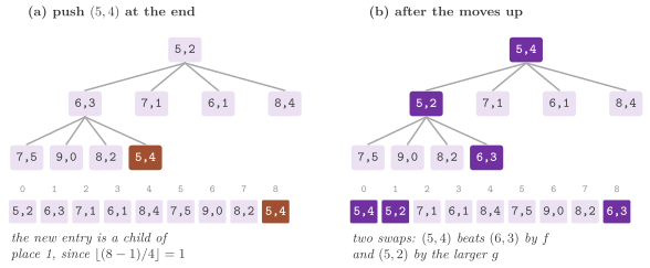
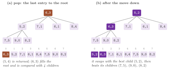
A binary heap keeps \(n\) entries in an array, the entry in the place \(i\) being not worse than its children in the places \(2i + 1\) and \(2i + 2\); the first entry is in the place 0. A \(d\)-ary heap has \(d\) children per node, in the places \(d i + 1, \ldots, d i + d\), and the parent of the place \(i > 0\) is the place \(\lfloor (i - 1) / d \rfloor\) (cf. Johnson [158]). Here "better" is a strict weak order on the keys of the entries, i.e., a strict order whose incomparability is transitive (as the order of A\(^*\) below, in which the entries with the same \(f\) and \(g\) are incomparable), and "not worse" its negation, which is then transitive too. A push puts the new entry in the place \(n\) and moves it up, past its parent as long as it is better (Figure 3.1). A pop takes the entry of the place 0, moves the last entry there and moves it down, past the best of its children as long as that child is better (Figure 3.2). The default heap moves a hole rather than swapping, i.e., it shifts each parent (or child) into the hole and writes the moving entry once, at its final place.
Algorithm 3.2 (Push and pop in a \(d\)-ary heap \(A[0 .. n − 1]\)).
 1  procedure PUSH(A, x)
 2     i ← n;  n ← n + 1
 3     while i > 0 and x is better than A[(i − 1) div d] do
 4        A[i] ← A[(i − 1) div d];  i ← (i − 1) div d
 5     A[i] ← x

 1  function POP(A)                                    ▷ n ≥ 1
 2     r ← A[0];  x ← A[n − 1];  n ← n − 1;  i ← 0
 3     if n = 0 then return r
 4     loop
 5        if d i + 1 ≥ n then break                 ▷ i is a leaf
 6        c ← the best of A[d i + 1 .. min(d i + d, n) − 1]
 7        if A[c] is not better than x then break
 8        A[i] ← A[c];  i ← c
 9     A[i] ← x
10     return r
Proposition 3.3 (Correctness and cost of a \(d\)-ary heap). Algorithm 3.2 keeps the heap order, i.e., no entry is better than its parent; hence \(A[0]\) is an entry of which no other is better. Let \(k = \lceil \log_d ((d - 1) n + 1) \rceil - 1\) be the depth of the place \(n - 1\), with \(n\) the entries after a push or before a pop. A push makes at most \(k\) comparisons and a pop at most \(d k\), i.e., \(O(\log_d n)\) and \(O(d \log_d n)\).
Proof. Order. In PUSH, let the hole be at \(i\); the invariant of the loop is that the array, with the hole filled by any entry not worse than the entries of its subtree and not better than its parent, is in heap order. It holds at the start, since the hole is a new leaf, and line 4 keeps it: the parent moved into the hole is not worse than the entries below it (it was their ancestor) and \(x\) is better than it. When the loop stops, \(x\) is not better than the parent of the hole, and it is better than the entries moved below it, which were already not worse than the rest of the subtree. In POP the argument is symmetric: line 8 moves into the hole the best child, which is not worse than its siblings and than its own subtree, and line 9 writes \(x\) where no child is better than it. Since the order is transitive along the paths to the root, \(A[0]\) is an entry of which no other is better. Cost. The levels \(0, \ldots, \ell\) of a \(d\)-ary heap hold \((d^{\ell + 1} - 1) / (d - 1)\) places, and hence the place \(n - 1\) has the depth \(k\) of the statement. PUSH makes one comparison per level that the entry climbs, at most \(k\); POP makes, per level that the hole descends, at most \(d - 1\) comparisons to find the best child and one with \(x\), i.e., at most \(d k\). \(\square\)
In the default set, HeapOpenList is a \(d\)-ary heap with \(d = 4\). Its
items are the triples \((f, g, u)\), i.e., they carry \(f\) and \(g\) next to
the pointer to the node, and hence a comparison never follows the
pointer. The order is that of A\(^*\): the item \((f_1, g_1, u_1)\) is better
than \((f_2, g_2, u_2)\) if \(f_1 < f_2\), or \(f_1 = f_2\) and \(g_1 > g_2\);
two items with the same \(f\) and \(g\) are not better than each other, and
they leave the heap in an order that the operations do not fix. With \(d
= 4\) the heap has half the levels of a binary heap, and by Proposition
3.3 a push makes half the comparisons, while a pop makes 4 comparisons
per level against 2, on half the levels, i.e., about as many in all.
Furthermore, with integer costs an item takes 16 bytes. The four
children of a place \(i\) are thus the 64 consecutive bytes from the
offset \(16 (4i + 1) = 64 i + 16\), and in an array aligned to a line
of 64 bytes (as the arrays on huge pages are, cf.
§3.7) they straddle two lines of cache
(an array shifted by three places
would align them on one), and the descent of a pop reads at most two
lines per level, on half the levels of a binary heap. Also, the array of
a large heap is allocated on huge pages, and the walk from the root to a
leaf, whose places are far apart, then does not miss the translation
lookaside buffer at each level. In the set std the heap is the binary
heap of std::priority_queue, and that of the set boost is the 4-ary
boost::heap::d_ary_heap. All three use the same order, and they may
differ only in the order of the items with the same \(f\) and \(g\).
3.3 The two-level bucket queue¶
With integer costs and a bounded range of \(f\), a priority queue can do
without comparisons: the queue of Dial [65]
keeps an array of buckets indexed by the key, and it finds the least key
by a scan that moves forward. The order of A\(^*\) has two keys, the least
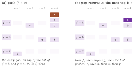
\(f\) and then the largest \(g\). Accordingly, BucketOpenList, the default
OPEN for integer costs, nests two levels of buckets, as the nested bucket
queue of Burns et al. [4] (which they
distinguish from the 2-level bucket queue of
[10], meant to shrink the array when the
values of \(f\) are many): an array of layers indexed by \(f\), the layer
\(f\) holding the entries with that \(f\) in a set of LIFO lists, one per
value of \(g\) (Figure 3.3). Two bounds
make the scans short: \(\mathit{minF}\), below which no layer has entries,
and, in each layer \(L\), \(\mathit{topG}(L)\), above which no list of
the dense array of the layer (see below) has entries.
The lists of a layer need care. An array of heads indexed by \(g\) costs \(\Theta(G)\) to rebuild, with \(G\) the largest \(g\) of the layer, and on a grid \(g\) grows to thousands while a layer holds few entries. The default queue therefore keeps in a dense array the heads of the lists of \(g < D = 256\) (the first \(S = 4\) of them inside the layer itself), and those of \(g \ge D\) as a sorted vector of at most \(R = 64\) runs \((g, \mathit{head})\), the last of which is the top of the layer; a layer that has runs is sparse. A push of some \(g \ge D\) into a layer that already has \(R\) runs turns it dense, i.e., it moves the heads of its runs into the dense array, which then covers all its values of \(g\), and the layer stays dense until it empties, when it frees the part of the array of \(g \ge S\) and resets \(\mathit{topG}\) to 0. The items lie in one vector of cells, each with the index of the next cell of its list, and the cells freed by a pop form a free list that a push takes from first; hence a push or a pop calls no allocator once the vector has reached the largest size of the queue.
Algorithm 3.3 (The two-level bucket queue; \(L\) is the layer of \(f\), \(v\) its runs, \(\mathit{head}_L[g]\) its dense array).
 1  procedure PUSH(x, f, g)
 2     if g ≥ D and L is not dense then
 3        if |v| = R then MAKE-DENSE(L)                ▷ L is now dense
 4        else insert x at the head of the run of g in v
 5                    ▷ a new last run if g > the last g of v, else the
 6                    ▷ run of g found, or inserted, by binary search
 7     if g < D or L is dense then
 8        insert x at the head of the list head_L[g]
 9        if L had no entry or g > topG(L) then topG(L) ← g
10     count(L) ← count(L) + 1
11     if the queue was empty or f < minF then minF ← f

 1  function FRONT()                                   ▷ queue not empty
 2     while count(the layer of minF) = 0 do minF ← minF + 1
 3     L ← the layer of minF
 4     if v = ∅ then
 5        while head_L[topG(L)] = nil do topG(L) ← topG(L) − 1
 6        return the head of head_L[topG(L)], with (minF, topG(L))
 7     return the head of the last run of v, with (minF, its g)

 1  function POP()
 2     (x, f, g) ← FRONT();  unlink x from its list; its cell to the free list
 3     if x came from the last run of v and that run is now empty then
 4        drop the run
 5     count(L) ← count(L) − 1
 6     if count(L) = 0 then free head_L[S ..];  topG(L) ← 0
 7     return (x, f, g)

 1  procedure MAKE-DENSE(L)
 2     G ← the last g of v;  extend head_L to the places 0 .. G
 3     for each run (g', h') of v do head_L[g'] ← h'
 4     v ← ∅;  topG(L) ← G
In the following we write \(f_{\max}\) for the largest \(f\) pushed and \(G_L\) for the largest \(g\) pushed into the layer \(L\).
Lemma 3.4 (The invariants of the bucket queue). After each operation of Algorithm 3.3: (i) no layer below \(\mathit{minF}\) has an entry; (ii) the runs of a layer are sorted by increasing \(g\), all of \(g \ge D\) and with entries, there are at most \(R\) of them, and a dense layer has none; (iii) in a layer that is not dense every entry of \(g \ge D\) is in a run and every other one in the dense array, and in a dense layer all are in the dense array; (iv) no list of the dense array above \(\mathit{topG}(L)\) has entries. Hence FRONT returns an entry of the least \(f\), of the largest \(g\) among those, and the last one pushed among those with the same \(f\) and \(g\).
Proof. (i) A push lowers \(\mathit{minF}\) to its \(f\) if \(f\) is smaller (or sets it if the queue was empty), and FRONT moves it forward only past empty layers. (ii) A run is appended only with a \(g\) larger than the last one, or inserted at its sorted position; a run is dropped when its list empties; MAKE-DENSE empties \(v\), and it is called when \(|v| = R\), before a further run would be created. (iii) This follows from the tests of lines 2 and 7 of PUSH and from MAKE-DENSE, which moves all the runs. (iv) Line 9 of PUSH raises \(\mathit{topG}\) to every \(g\) pushed into the dense array (and sets it to \(g\) when the layer was empty), MAKE-DENSE sets it to the largest \(g\) of the layer, line 5 of FRONT lowers it only past empty lists, and line 6 of POP resets it only when the layer is empty. For the last claim, by (i) the layer of \(\mathit{minF}\) after line 2 of FRONT is the least nonempty one; if it has runs, by (ii) and (iii) the last run holds the largest \(g\) of the layer, since all the entries of the dense array have \(g < D\); otherwise, by (iv), line 5 stops at the largest nonempty list. The lists are LIFO, since an entry is inserted at the head and taken from it. \(\square\)
We now give the cost. The two scans (lines 2 and 5 of FRONT) are paid by the moves of the bounds in the opposite direction, which is the argument of the following proposition.
Proposition 3.5 (The cost of the bucket queue). (i) Over any sequence of operations, the steps of the scan of line 2 of FRONT are at most \(f_{\max} + 1\) plus the sum of the decreases of \(\mathit{minF}\) at line 11 of PUSH, and the steps of the scan of line 5 in a layer are at most the sum of the raises of \(\mathit{topG}\) in it (line 9 of PUSH and line 4 of MAKE-DENSE). (ii) Besides the scans, a push costs \(O(1)\) amortized time if it goes to the dense array or to the end of the runs, and \(O(\log R + R)\) if it inserts a run in the middle; a MAKE-DENSE costs \(O(G_L)\); a pop costs \(O(1)\) besides FRONT, plus \(O(G_L)\) for the release of a dense array at line 6. (iii) Hence, if the least \(f\) never decreases between two pops (as in A\(^*\) with a consistent heuristic, by Theorem 2.13), all the pops of a search cross at most \(f_{\max} + 1\) layers; and if all the pushes into a layer that is never dense precede its first pop, its scan of line 5 makes at most \(D - 1\) steps until it empties.
Proof. (i) \(\mathit{minF}\) never exceeds \(f_{\max}\) while the queue holds an entry, increases only by one at line 2, and otherwise changes only at line 11; hence its increases are at most \(f_{\max}\) plus its decreases (a push into the empty queue may also raise it, which costs no step). The same argument holds for \(\mathit{topG}(L)\), which decreases only at line 5 and starts at the \(g\) of the first push at each filling of the layer. (ii) The dense array grows by doubling, which costs \(O(1)\) amortized per element, and a cell comes from the free list or from the end of a vector that doubles; the binary search over at most \(R\) runs costs \(O(\log R)\) and the insertion shifts at most \(R\) runs; MAKE-DENSE extends the array to \(G_L + 1\) places, and the release frees as many. (iii) Under the first hypothesis no push lowers \(\mathit{minF}\) after the first pop. Under the second, the raises of \(\mathit{topG}\) in a dense array of \(g < D\) total at most \(D - 1\), since \(\mathit{topG}\) only increases until the first pop. \(\square\)
Thus, in A\(^*\) with a consistent heuristic the scan of the layers costs
\(O(f_{\max})\) over the whole search. Within a layer, the pushes and the
pops interleave, since the expansion of an entry of the least layer
pushes its children of equal \(f\) into the same layer. Each such push
raises \(\mathit{topG}\) by at most \(c(u, v)\) above the \(g\) of the entry
just popped, at which FRONT had left \(\mathit{topG}\), and therefore the
scan of line 5 costs at most \(D - 1\) steps for the pushes made before
the first pop of the layer plus \(c(u, v)\) per child pushed into it
afterwards. Without the first hypothesis, as in a worker of HDA\(^*\),
whose least layer empties and fills again each time the nodes sent by
the other workers arrive, the bound \(\mathit{minF}\) moves back, and by
(i) the scan may cross a layer many times. Also, a sequence that
alternates a push of a large \(g < D\) with its pop, in a layer that keeps
an entry of \(g = 0\), costs a scan of \(\Theta(D)\) per pop. The runs avoid
this for the values \(g \ge D\): their top is the last run, found without
a scan, and a dense array over them is built only after \(R\) distinct
values \(g \ge D\) have been pushed into the layer, i.e., its \(O(G_L)\)
is paid by at least \(R\) pushes, whereas a dense array alone would cost
\(\Theta(G_L)\) at each filling, even of one entry. The memory is that
of the \(f_{\max} + 1\) layers, of the cells (as many as the largest size
of the queue), of the dense arrays (at most \(D\) heads per layer that is
not dense, and \(G_L + 1\) per dense layer) and of at most \(R\) runs per
sparse layer. It grows with the range of the keys rather than with
the entries, and the queue is therefore used only for integer costs. We
remark that the cells are indexed by 32-bit integers, and the queue
therefore holds fewer than \(2^{32} - 1\) entries at a time. The sets
std and boost, which have no bucket queue, use the heap for all the
cost types.
The test open checks both OPEN lists against an ordered multiset of
the pairs \((f, -g)\) on random sequences of 20000 pushes and pops in
which the least \(f\) moves back below the \(f\) of the last pop, as in a
worker of HDA\(^*\), with \(g\) up to 200 and up to 2000, i.e., on both
sides of \(D\).
Status — planned. The radix heap of Ahuja et al. [160], which needs only that no key pushed be smaller than the last key popped (the case of A\(^*\) with a consistent heuristic) and costs \(O(\log C)\) amortized time per extraction for keys in a range of \(C\), is not an OPEN list of the library; the bucket queue covers the integer costs of its domains, and the heap the others.
3.4 Packed keys¶
The parallel searches whose OPEN is shared or relaxed (MultiQueue A\(^*\)
and PA\(^*\)SE of Chapter 8) compare the keys
of the entries as single machine words, and a comparison, or an atomic
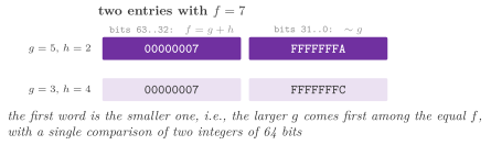
read of a key, is then one instruction. For integer costs, packed_fg
(Node.h:114-120) puts \(f = g + h\) in the high half of a
word of 64 bits and the complement of \(g\) in the low one.
Algorithm 3.4 (The packed key of \((g, h)\)).
The second term is the complement of \(g\) in 32 bits, which the code computes as the bitwise negation of \(g\) masked to its low 32 bits.
Lemma 3.6 (The order of the packed keys). Let \(0 \le g_i\), \(0 \le h_i\) and \(g_i + h_i < 2^{32}\) for \(i = 1, 2\), and let \(k_i\) be the packed key of \((g_i, h_i)\). Then \(k_1 < k_2\) if and only if \(f_1 < f_2\), or \(f_1 = f_2\) and \(g_1 > g_2\).
Proof. The key is \(k_i = 2^{32} f_i + (2^{32} - 1 - g_i)\), and since \(0 \le g_i \le f_i < 2^{32}\) (here \(h_i \ge 0\) is used) the low half lies in \([0, 2^{32})\). Hence the comparison of the keys is that of the high halves, and for equal high halves that of the low ones, i.e., the comparison of \(f\) and then the reverse comparison of \(g\). \(\square\)
The sum \(g + h\) is computed in the cost type before it is widened, and with a signed 32-bit cost the range is therefore \(g + h < 2^{31}\), the largest value of the type. Figure 3.4 shows two keys of the same \(f\): the one of the larger \(g\) is the smaller word, and comes first.
3.5 Breaking the ties¶
Both OPEN lists break the ties of \(f\) in favor of the larger \(g\), i.e., of the smaller \(h\), since \(g = f - h\) when \(f\) is fixed; ordering by the least \(h\) among the least \(f\), as some textbooks put it, is the same rule. We now make precise what the choice changes, with a consistent heuristic and the notation of §2.6.
Proposition 3.7 (The ties change only the last layer). With a consistent heuristic and any rule for the ties, A\(^*\) expands the same nodes with \(g^*(u) + h(u) < C^*\) and none with \(g^*(u) + h(u) > C^*\); the rules differ only in the nodes of the last layer, \(g^*(u) + h(u) = C^*\), that they expand before a goal.
Proof. The claim is Theorem 2.14, whose proof does not depend on the order of the entries with equal keys. \(\square\)
Proposition 3.8 (The ties with a perfect heuristic). Let the costs be at least some \(\varepsilon > 0\) and \(h = h^*\), and let a goal be reachable. With the ties of \(f\) broken in favor of the larger \(g\), A\(^*\) expands the nodes of one optimal path from \(s_0\) to a goal, and no other node.
Proof. Since \(h = h^*\), a node \(v\) has \(g^*(v) + h(v) = C^*\) if and only if it lies on an optimal path, and \(g^*(v) + h(v) > C^*\) otherwise; the heuristic is consistent (\(h^*(u) \le c(u, v) + h^*(v)\) on every edge), and by Theorem 2.14 no node of the second kind is expanded. Let \(x_0 = s_0, x_1, \ldots\) be the nodes selected from entries that are not stale, in their order. We show by induction on \(j\) that, as long as \(x_j\) is not a goal, (a) \(x_{j+1}\) is a successor of \(x_j\) on an optimal path, with \(g(x_{j+1}) = g(x_j) + c(x_j, x_{j+1}) > g(x_j)\), and (b) when \(x_j\) is selected, every entry of key \(C^*\) in OPEN has \(g \le g(x_j)\); (b) holds for \(x_0\), the only entry. Let (b) hold for \(x_j\), not a goal. By Theorem 2.13, \(g(x_j) = g^*(x_j)\), and since \(h(x_j) = h^*(x_j)\) is finite, \(x_j\) has a successor \(y\) on an optimal path, with \(g^*(y) = g(x_j) + c(x_j, y) > g(x_j)\). The node \(y\) is not closed: the nodes closed so far are \(x_0, \ldots, x_j\), whose values of \(g\) are at most \(g(x_j)\) by (a), while a closed node has \(g = g^*\) (Theorem 2.13). Nor did \(y\) have, before the expansion, the entry \((C^*, g^*(y), y)\), whose \(g\) exceeds \(g(x_j)\), against (b). Hence the expansion of \(x_j\) sets \(g(y) = g^*(y)\) and pushes that entry (line 13 or 16 of Algorithm 2.2). After the expansion, every entry has a key at least \(C^*\); the entries of key \(C^*\) are those that were there, with \(g \le g(x_j)\), and those just pushed, which have \(g = g(x_j) + c > g(x_j)\) and belong to successors on optimal paths, and none of the latter is stale, since a value \(g^*\) cannot be improved. The next entry selected has the largest \(g\) among those of key \(C^*\), which is (a) and (b) for \(j + 1\). Since the values of \(g\) increase by at least \(\varepsilon\) from each \(x_j\) to the next and are at most \(C^*\), the sequence reaches a goal after at most \(C^* / \varepsilon\) steps; the selected nodes form a path from \(s_0\), each the successor of the previous one on an optimal path, and it ends at the first goal selected. \(\square\)
In words, with the ties in favor of the larger \(g\) the search dives along the last layer, and with an exact heuristic it expands only the \(d + 1\) nodes of the path it returns, \(d\) being its number of edges; an informative heuristic, exact on part of the last layer, gives a similar dive on that part (an observation, not a theorem). Conversely, the opposite rule does the reverse: since \(h \ge 0\), a goal \(t\) has the largest \(g\) of the last layer, \(g(t) = C^*\), and with the ties in favor of the smaller \(g\) it is selected only when no other entry of key \(C^*\) is left in OPEN, i.e., after all the nodes of the last layer that are generated before it have been expanded. On the grid of Figure 2.6 the two rules expand 8 and 31 of the 31 cells of the last layer; on the domains with unit costs and few values of \(f\), such as the sliding-tile puzzles, the last layer may hold a large part of the nodes, and the experiments of Burns et al. [4] report that the larger \(g\) is the better rule. Among the entries with the same \(f\) and \(g\), the bucket queue takes the last one pushed (Lemma 3.4), which follows the most recent path, while the heaps take any of them; this last order differs among the three sets of §3.12, which therefore may expand different nodes of the last layer, and only of it.
With real costs, two values of \(g\) that are sums of the same edge costs
in another order may differ in their last bits, and a node closed with
the larger one would be reopened with the smaller, and its subtree
expanded again, although the two paths have the same cost; therefore, in
every search of the library a path counts as cheaper only by more than \(\tau \max\{1, g(v)\}\), \(\tau =
10^{-9}\) (cheaper() and cost_slack() of
Node.h:134-148), so that the cost returned exceeds \(C^*\)
by at most \(\tau \max\{1, C^*\}\) per edge of the path; on the random grid
1 of 60 by 60 cells with 8 moves A* thus selects 252 nodes instead of 276,
24 of which were reopened by the rounding alone. The order of OPEN,
instead, compares \(f\) and \(g\) exactly, since a comparison up to a
tolerance is not transitive and would break the order of a heap; hence,
the values of \(f\) equal but for the rounding are taken in the order of
their last bits, and the ties among them are not broken by \(g\).
3.6 CLOSED: a hash table with open addressing¶
CLOSED is a dictionary from the generated states to their nodes, with no
removal, since a search never forgets a state. The default NodeTable
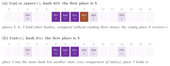
is a hash table with open addressing and linear probing: its places
are an array of \(m = 2^k\) cells, each holding the pointer to a node
(\(\mathrm{nil}\) in an empty place) and the 64-bit hash of its state, and
a state is looked for from its first place onward, along consecutive
places taken modulo \(m\), up to its place or an empty one (Figure
3.5). Two choices make a probe cheap.
The hash is stored, and hence a probe compares two states only when
their hashes are equal, and a growth moves the places without touching
the nodes. Also, the places are consecutive in memory, and a probe
sequence reads one or two lines of cache instead of following the
pointers of a list.
The first place of a hash \(x\) in a table of \(2^k\) places is
i.e., the top \(k\) bits of the product of \(x\) by \(M\), which is the multiplicative hashing of Knuth with the golden ratio (Fibonacci hashing, cf. section 6.4 of [157]). The low bits of \(x\) are often regular: in a worker of HDA\(^*\), for instance, all the states have the same \(x \bmod p\), and a table that took the low \(k\) bits of \(x\) would use one place in \(p\). The product, instead, spreads all the bits of \(x\) into its top bits, and the states of a worker fill its whole table.
Algorithm 3.5 (The lookup with insertion in CLOSED; \(S[0 .. m − 1]\) the places, \(n\) the nodes stored).
 1  function FIND-OR-INSERT(s, x, make)            ▷ x the hash of s
 2     i ← the top k bits of (x · M) mod 2^64      ▷ m = 2^k
 3     while S[i].node ≠ nil do
 4        if S[i].hash = x and the state of S[i].node = s then
 5           return (S[i].node, false)
 6        i ← (i + 1) mod m
 7     u ← make();  S[i] ← (x, u);  n ← n + 1
 8     if 10 n > 7 m then GROW
 9     return (u, true)

 1  procedure GROW
 2     T ← S;  m ← 2 m;  k ← k + 1;  S ← m empty places
 3     for each place (x, u) of T with u ≠ nil do
 4        i ← the first place of x
 5        while S[i].node ≠ nil do i ← (i + 1) mod m
 6        S[i] ← (x, u)
The lookup without insertion, find, is lines 2 to 6 with \(\mathrm{nil}\)
returned at the first empty place, and prefetch( x ) issues a prefetch of
the place of line 2. Thus the table doubles when its load factor
\(\alpha = n / m\) would exceed \(7/10\), and the insertion is done by the same
probe that finds the state absent, with one inspection only.
Lemma 3.9 (Correctness of the linear probing).
After each operation of Algorithm 3.5, every node stored is in a place
reached from the first place of its hash along occupied places only, and
the load factor is at most \(7/10\). Hence FIND-OR-INSERT returns the node
of \(s\) if \(s\) is stored, and otherwise inserts it, and find returns
\(\mathrm{nil}\) exactly for the states not stored.
Proof. A place, once occupied, is never emptied, since there is no removal; hence the places between the first place of a node and its place, all occupied when it was inserted, stay occupied. GROW reinserts every node by the same probe in an empty table, which gives the property again. The load factor is at most \(7/10\) after line 8, and at most \(7/20\) after a doubling. Since \(\alpha < 1\), the table has an empty place, and the loop of line 3 ends. If \(s\) is stored, its place is on the probe sequence from its first place before any empty place, and the loop meets it (the hash compared at line 4 is the one stored with it); if \(s\) is not stored, the loop reaches an empty place. \(\square\)
Lemma 3.10 (The size for \(n\) nodes). A table built
with slots_for( n ) places, the least power of 2, at least 16, with
\(10 n \le 7 m\), holds \(n\) nodes without growing.
Proof. The constructor takes the least power of 2 that is at least the
given number (and at least 16), here slots_for( n ) itself, and hence
\(7 m \ge 10 n \ge 10 n'\) after each of the first \(n\) insertions, \(n'\) the
nodes stored; the test of line 8 then fails for each of them. \(\square\)
SearchOptions::expected_nodes gives the number \(n\) of nodes for which
AStar builds its table with slots_for( n ) places at the start of a search
(§2.3), and by Lemma 3.10 a search that stores at
most that many nodes never grows its table; otherwise the table starts at 1024
places. We recall the classical analysis of linear probing for the cost of a
lookup.
Proposition 3.11 (The cost of CLOSED). With hash values independent and uniformly distributed, and a load factor \(\alpha < 1\), a successful lookup inspects about \(\frac{1}{2}\bigl(1 + \frac{1}{1 - \alpha}\bigr)\) places on average and an unsuccessful one about \(\frac{1}{2}\bigl(1 + \frac{1}{(1 - \alpha)^2}\bigr)\); with \(\alpha \le 7/10\) these are at most about 2.2 and 6.1 places. The doublings cost \(O(1)\) amortized time per insertion, besides the probes of the reinsertions, without any hypothesis on the hashes.
Proof. The two averages are the classical results on linear probing (section 6.4 of [157]), and at \(\alpha = 7/10\) they are \(\frac{1}{2}(1 + 10/3) \approx 2.17\) and \(\frac{1}{2}(1 + 100/9) \approx 6.06\). A doubling from \(m\) to \(2m\) places scans the \(m\) places, writes \(2m\) empty ones and reinserts at most \(\frac{7}{10} m + 1\) nodes, i.e., it costs \(O(m)\) besides the probes of the reinsertions; it follows at least \(\frac{7}{20} m\) insertions since the previous doubling, i.e., at least \(\lfloor 7m/10 \rfloor - \lfloor 7m/20 \rfloor \ge 7m/20 - 1\) of them (and \(\lfloor 7m/10 \rfloor - 1\) before the first one, from an empty table), to which its cost is charged, \(O(1)\) each for \(m \ge 16\). \(\square\)
We remark that the hypothesis on the hashes is an assumption on the
member hash of the domain, which the library does not check: a domain
whose hashes collide often makes the probe sequences longer, and the
averages above then do not hold. The unsuccessful lookups are those of
the new states, i.e., one per node stored, and the successful ones
those of the duplicates. A probe sequence of 6 places of 16 bytes spans
96 bytes, i.e., two or three lines of cache. In the set std, CLOSED is
a std::unordered_map (a table of chains) whose key is the pair of the
state and of its hash, the hash of the key being the one stored in it
and the equality that of the states; the map thus does not evaluate the
hash of the domain again, and try_emplace gives the insertion with one
lookup. Its prefetch does nothing, since a table of chains cannot
prefetch a bucket. In the set boost, CLOSED is
boost::unordered_flat_map, a table with open addressing, with the same
key, reserved for \(7/10\) of its places as the default one; its
prefetch does nothing either. We remark that ADS built with the headers
of Boost (ADS_WITH_BOOST) would put the places of the table of the set
ads in a boost::unordered_flat_set, which cannot be prefetched; PBeFS
defines ADS_POINTERTABLE_BOOST=0, so that the table is the one above
with every build of ADS, since it is the faster of the two on large
searches, where most of the lookups miss the cache
(§3.8).
3.7 The arena of the nodes¶
A node (Node, Node.h:73-89) has the following fields, in
this order: the state; \(g\), the cost of the best path found from \(s_0\); \(h\);
the pointer to its parent on that path (\(\mathrm{nil}\) at the root); the
flag closed, set when the node is expanded with its current \(g\) and
cleared when \(g\) improves; the flag expanded, set at the first
expansion and never cleared, by which the re-expansions are counted
(§2.3); the operator that generated the
state, of one byte (no_op at the root, used only by an
OperatorDomain); and a 32-bit key of the state for its owner, used
only by the distributions of the parallel searches that follow the moves
(Chapter 9). The member f() returns
\(g + h\). With a state of one word and integer costs of 32 bits, a node
takes 32 bytes: 8 for the state, 4 each for \(g\) and \(h\), 8 for the
parent, and 8 for the two flags, the operator and the key, which fit in
what would otherwise be the padding after the flags. The infinite cost
of a cost type, which stands for no incumbent and for the bound of a
search not yet cut, is infinite_cost() (Node.h), i.e., the
infinity of a floating-point type and the largest value of an integer one; the
path to a goal is rebuilt by trace_path, which follows the parents
from the goal and reverses the states.
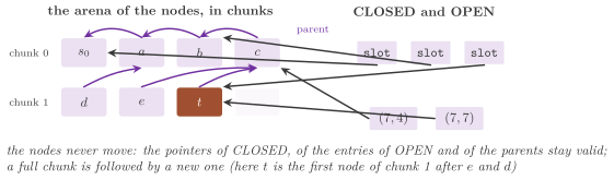
The nodes are allocated from an arena (NodePool): a block of \(B =
2^{16}\) nodes is taken from the system when the previous one is full,
and a node is allocated by advancing an index in the block, without a
call to the allocator (Figure 3.6).
Algorithm 3.6 (The allocation of a node from the arena).
1  function ALLOCATE()
2     if there is no block or used = B then
3        append a new block of B nodes;  used ← 0
4     used ← used + 1
5     return the place used − 1 of the last block, value-initialized
Proposition 3.12 (The arena). The address of a node never changes until the arena is destroyed, a call of ALLOCATE costs \(O(1)\) time besides the allocation of a block once in \(B\) calls, and \(N\) nodes take the memory of \(\lceil N / B \rceil\) blocks, i.e., of at most \(B - 1\) nodes more than \(N\).
Proof. A block is never moved nor freed before the arena, and each node is built in place in a block (line 5); the other claims follow from line 2, which takes a new block only when the last one is full. \(\square\)
The arena has some consequences. The pointers to a node (from CLOSED,
from the entries of OPEN and from its children as their parent) stay
valid until the end; hence CLOSED and OPEN can store pointers, and
neither moves a node. Also, the nodes made one after another are next
to each other in memory, and the children of a node, which are made
together, often share lines of cache; furthermore, a node costs no
header of the allocator. With nodes of 32 bytes a block is 2 MB, i.e.,
one huge page. The price is that the nodes are freed only all together,
at the end of the search, and that the arena does not reuse the nodes
of the states that are closed for good. In the set std the nodes are
kept in a std::deque, whose emplace_back does not move the nodes
already there either, and in the set boost in a boost::object_pool.
The blocks of the arena, the places of CLOSED and the array of a large heap of the default set are requested from the operating system as huge pages where possible: a request of at least 2 MB is aligned to 2 MB, rounded up to whole huge pages and, on Linux, advised to the kernel for the transparent huge pages, which the kernel may ignore; a smaller request goes to the standard allocator. A structure whose places are reached in no useful order, as those of CLOSED by hashes, then misses the translation lookaside buffer once per 2 MB instead of once per 4 KB page, and its memory is faulted in a huge page at a time.
3.8 Prefetching the lookups¶
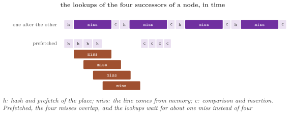
On a large search, CLOSED is much larger than the cache, and the place of a successor lies at an address that the hash makes random; almost all the lookups then miss the cache, and the time of an iteration is dominated by \(b\) misses. For this reason, the sequential A\(^*\) splits the expansion of lines 9 to 16 of Algorithm 2.2 in two passes.
Algorithm 3.7 (The expansion of \(u\) in two passes).
 1  procedure EXPAND(u)
 2     K ← ∅                                    ▷ the successors of u
 3     for each successor v of u do              ▷ the first pass
 4        x ← hash(v);  prefetch the first place of x in CLOSED
 5        append (v, c(u, v), h(v), x) to K
 6     for each (v, c, h(v), x) in K do         ▷ the second pass
 7        (w, new) ← FIND-OR-INSERT(v, x, a node of v with g(u) + c)
 8        if new then push w in OPEN
 9        else if g(u) + c < g(w) then
10           g(w) ← g(u) + c;  parent(w) ← u;  w is not closed
11           push w in OPEN
The first pass generates all the successors, computes their hashes and issues a prefetch of the first place of each hash into the cache, without waiting for it. The second does the lookups, by which time the lines are on their way or already there. A prefetch is a hint to the processor, which changes no value; hence Algorithm 3.7 makes the same lookups, insertions and pushes as lines 9 to 16 of Algorithm 2.2, in the same order. Its gain, on the other hand, is not a property that we can prove: on a processor that serves several misses at a time, the misses of the \(b\) lookups overlap (Figure 3.7), and the iteration waits for about one miss instead of \(b\), while on one that serves a single miss at a time nothing is gained. Also, the parallel searches do the same with the batches of nodes they receive (Chapter 9), whose lookups are independent of each other. The price is the memory of \(K\), i.e., \(b\) records, reused from one expansion to the next.
3.9 Perfect hashing¶
A perfect hash of the states is an injective map of the states to the
integers, and a minimal one maps \(n\) states onto \([0, n)\). A domain with a
perfect hash models the concept PerfectHashDomain
(Domain.h:230), whose perfect_hash( s ) the distribution
HDA\(^*\)[P] of Burns et al. [3] uses to assign the
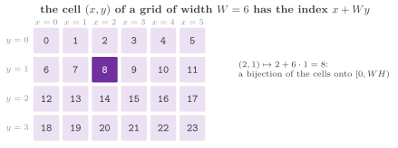
states to the workers (Chapter 9). On a grid of
width \(W\) and height \(H\), the cell \((x, y)\), with \(0 \le x < W\) and
\(0 \le y < H\), has the index \(x + W y\), and the state of the domain Grid is
that index itself (Figure 3.8).
Lemma 3.13 (The perfect hash of a grid). The map \((x, y) \mapsto x + W y\) is a bijection of the cells of a grid of width \(W\) and height \(H\) onto \([0, W H)\), i.e., a minimal perfect hash.
Proof. Since \(0 \le x \le W - 1\), the index \(i = x + W y\) satisfies \(W y \le i \le W y + W - 1\), and hence \(y = \lfloor i / W \rfloor\) and \(x = i \bmod W\) are determined by \(i\), i.e., the map is injective. Its values lie in \([0, W (H - 1) + W - 1] = [0, W H)\), and the \(W H\) cells are thus mapped injectively onto these \(W H\) integers. \(\square\)
The explicit graphs use the index of the node, and the traveling salesperson, the vacuum world and the missionaries and cannibals pack their states into words that are their perfect hashes. On the permutations, the lexicographic ranking of §5.4 is a minimal perfect hash of the placements of a pattern, which the pattern databases use as the indices of their tables (the ranking of Myrvold and Ruskey [34] would serve as well, cf. §5.4).
With a minimal perfect hash and a known number of states, CLOSED could be a plain array indexed by it, with no probe at all; the library keeps the hash table for all the domains, which does not depend on the range of the hash nor on the number of states, and leaves the perfect hashes to the distributions and to the tables of the heuristics.
3.10 Transposition tables¶
A transposition table is a CLOSED that may forget: it has a fixed number of places, and when it is full a new state replaces an old one by a replacement rule (e.g., the one with the smaller \(g\), or the one reached less often), or the new state is not stored. Such a table gives the depth-first searches, which keep no CLOSED, part of the duplicate detection of a graph search within a bounded memory: a state found in the table with a \(g\) not larger is not searched again (that this keeps IDA\(^*\) optimal is Proposition 4.10). With the stochastic node caching of Miura and Ishida [162], a state is stored with a probability \(p\) at each visit, the draws being independent; a state visited \(n\) times is then in the table with probability \(1 - (1 - p)^n\), since it is missing only if all the \(n\) draws fail, and the states reached by many paths, which are those whose detection saves the most, are stored with a high probability.
Status — planned. The library has no transposition table; its depth-first search, IDA\(^*\), detects only the move back to the parent (§2.9 and Chapter 4).
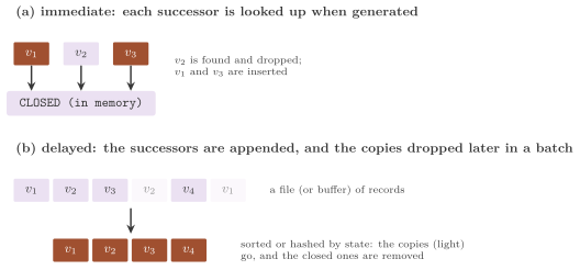
3.11 Immediate and delayed duplicate detection¶
The searches of Chapter 2 detect the duplicates
immediately: each successor is looked up in CLOSED when it is
generated, and it is dropped at once if its state is known with a \(g\)
that is not larger. A search with delayed duplicate detection instead
appends the successors to a buffer, or to a file on the disk, without
looking them up, and removes the copies later, in a batch, by sorting or
hashing the buffer and comparing it with the states already expanded
(Figure 3.9). The batch replaces the
random lookups by sequential passes, as the disk requires, and it lets
CLOSED live outside the memory. Its price is that the copies are stored
until the batch, and that the order of the expansions is that of the
batches, not of the single nodes. The search of Chapter
4 (DDDAStar) keeps its buckets in files
and detects the duplicates of a file at once, before expanding it, so
that each state is expanded at most once (Theorem
4.15); the test ddd checks it, and
checks that the records of a search that exhausts its buckets split,
with the root, into the states stored and the copies dropped.
3.12 The sets of data structures¶
The arena, CLOSED and the OPEN lists of A\(^*\) come from one of three
sets, chosen when the library is built (Structures.h): the
default one; that of the standard library, chosen by the macro
PBEFS_STRUCTURES_STD; and that of Boost, chosen by
PBEFS_STRUCTURES_BOOST. CMake defines the macro from its option
PBEFS_STRUCTURES, whose values are std, boost and the name of the
default set (the default; any other value stops the configuration), and
the makefile from PBeFSSTRUCT (std, boost, or empty for the
default set); defining more than one macro is an error.
Node.h, NodeTable.h, OpenList.h
and ConcurrentClosed.h then include the classes of the
set from structures/std/, structures/boost/ or the default directory, with
the same interface (the adjacency of the explicit graphs has a version in
structures/boost/ and in the default directory, that of the grids only
in the default one, and the other sets use the adjacency written in
ExplicitGraph.h and Grid.h); the sets are the
following.
| set | NodePool |
NodeTable |
HeapOpenList |
BucketOpenList |
|---|---|---|---|---|
| default | arena, huge pages | linear probing | 4-ary heap | two levels |
std |
std::deque |
std::unordered_map |
binary heap | binary heap |
boost |
object_pool |
unordered_flat_map |
4-ary heap | 4-ary heap |
The searches are the same with all the sets, and so is the order of
their expansions, but for the ties of \(f\) and \(g\) in OPEN, which the
sets break differently; by Proposition
3.7, with a consistent heuristic they
expand the same nodes but in the last layer, and the costs returned are
the same. A search is parametrized by its OPEN list at compile time,
and the function astar chooses it at run time by an OpenKind; their
declarations (AStar.h, here without the bodies) are
template< Domain D , class Open = std::conditional_t<
                      std::is_integral_v< cost_t< D > > ,
                      BucketOpenList< Node< state_t< D > , cost_t< D > > > ,
                      HeapOpenList< Node< state_t< D > , cost_t< D > > > > >
class AStar {
 public:
 explicit AStar( const D & domain , const SearchOptions & options = {} );
 [[nodiscard]] Solution< state_t< D > , cost_t< D > > solve( void ) const;
 };

template< Domain D >
[[nodiscard]] Solution< state_t< D > , cost_t< D > >
astar( const D & domain , OpenKind open = OpenKind::automatic ,
       const SearchOptions & options = {} );
with the kinds
/// the kind of OPEN list a search uses
enum class OpenKind {
 automatic ,  ///< buckets for integer costs, heap otherwise
 heap ,       ///< HeapOpenList
 buckets ,    ///< BucketOpenList (integer costs only)
 heap_low_g   ///< HeapOpenList with the ties to the smaller g [see
              ///< LowGOpenList]
 };
Thus AStar< D , Open > takes BucketOpenList by default for integer costs
and HeapOpenList otherwise; in astar, automatic and buckets give
BucketOpenList for integer costs, heap gives HeapOpenList, and with
costs that are not integers all three give HeapOpenList (a request of
buckets is then silently served by the heap). The SearchOptions are those
of Chapter 1, of which expected_nodes sizes
CLOSED (Lemma 3.10). The arena and CLOSED have no parameter, being those of
the set. Furthermore, the parallel searches use the same classes in each
worker, and their shared structures (e.g., the CLOSED of SPA\(^*\)) are
described in Chapter 8. We keep the standard
library and Boost to measure the searches against them, with the script of the
next section.
An example¶
The following example, a case of the tester, solves an instance of the
15-puzzle with the two OPEN lists chosen at run time and with the heap
chosen at compile time, the table of CLOSED being sized by
expected_nodes; all the costs are those of the instance, and the
automatic choice is the bucket queue, with the same expansions.
const FifteenPuzzle d( ki.board );
SearchOptions o;
o.expected_nodes = 1 << 20;                // CLOSED sized at the start
const auto b = astar( d , OpenKind::buckets , o );     // the buckets
const auto h = astar( d , OpenKind::heap , o );        // the heap
const auto a = astar( d , OpenKind::automatic , o );   // here the buckets
// the same choice at compile time, by the OPEN list of AStar
using NodeT = Node< state_t< FifteenPuzzle > , cost_t< FifteenPuzzle > >;
const auto e = AStar< FifteenPuzzle , HeapOpenList< NodeT > >( d , o )
               .solve();
3.13 Benchmark¶
Status — planned. The table of this section is not yet produced by the tables of the manual.
The script tools/bench/structures.sh runs
tools/AStarBench from three builds of the library, one per set
of data structures, on instances of growing size: the 15-puzzle in four bands
of the instances of Korf [7], by the nodes that
A\(^*\) expands (about \(10^5\), \(10^6\), \(10^7\) and above \(7 \cdot 10^7\)), and
random grids of 2000 to 20000 cells a side, with 35% of the cells blocked and 4
and 8 moves. Each instance is solved by the sequential A\(^*\) (with both
OPEN lists on the 15-puzzle) and by the parallel searches (by default
HDA\(^*\) with the Zobrist distribution, whose structures are those of
each worker, and SPA\(^*\), whose CLOSED is shared) on 1, 2, 4, 8 and 16
threads,
twice with each set, the sets taking turns so that a drift of the
machine falls on all of them; each run is a process of its own, pinned
to the cores and the memory of one node, and the two runs of a set are
its A/A. As in §2.16, the clock is that of
solve(), which does not include the reading of the instance nor the
construction of the domain. Since the expansions are the same for the
three sets but for the last layer, the comparison is one of time and of
memory per node.
3.14 Notes and references¶
The bucket queue for integer keys is due to Dial [65], and its nested use with two levels, the ties broken in favor of the larger \(g\) and the pruning of the move back to the parent in a fast A\(^*\) are studied by Burns et al. [4], who report the bucket queue to be faster than a binary heap on the sliding-tile puzzles (they update the position of a node in OPEN when its \(g\) improves, where the library uses the lazy deletion); the textbook of Edelkamp and Schrödl [10] treats the priority queues, the hash tables and the duplicate detection of the searches at length. The \(d\)-ary heaps go back to Johnson [158], the radix heap is due to Ahuja et al. [160], the linear probing and the multiplicative hashing are analyzed in section 6.4 of [157], and the arenas, i.e., the allocation by lifetime, are those of Hanson [159]. The delayed duplicate detection on the disk is that of Korf [40] and of the External A\(^*\) of Edelkamp, Jabbar and Schrödl [39], and the stochastic node caching that of Miura and Ishida [162]. With respect to [4], the library adds the prefetch of the lookups, the huge pages, and the sparse lists of the large values of \(g\) in the bucket queue, which keep the queue usable on the grids and in the workers of HDA\(^*\); it does not reuse the nodes of the closed states, which the arena keeps until the end, and it has neither the radix heap nor the transposition tables.
3.15 Exercises¶
Exercise 3.1 (ctest -R PBeFS.open). Show that the order of
BucketOpenList (least \(f\), then largest \(g\), then the last pushed)
and that of HeapOpenList agree on the pairs \((f, g)\) that they pop,
and explain why the test compares the pops with an ordered multiset of
the pairs \((f, -g)\) rather than of the entries.
Exercise 3.2 (ctest -R PBeFS.open). In a worker of HDA\(^*\) the
least \(f\) of OPEN may fall below the \(f\) of the last pop. Give a
sequence of \(m\) pushes and pops on which, by Proposition
3.5 (i), the scan of the layers costs
\(\Theta(m f_{\max})\), and explain what the sparse lists of the values
\(g \ge 256\) save in the same situation.
Exercise 3.3 (ctest -R PBeFS.astar). On the 8-puzzle, break the
ties of \(f\) by the least \(h\) and then by the largest \(h\), and compare the
nodes expanded; show by
Proposition 3.7 that the two rules
differ only in the last layer, and that the costs are equal, as the
test checks for the two OPEN lists of the library.
Exercise 3.4 (ctest -R PBeFS.mqa-thread). Prove Lemma
3.6 also when \(g + h\) reaches \(2^{32} -
1\), and show that it fails when \(g + h \ge 2^{32}\). Which representation
of the key should a domain whose costs exceed that range use? (MultiQueue
A\(^*\), whose test runs here, orders its queues by these keys.)
Exercise 3.5 (ctest -R PBeFS.hda-thread). Show, from Lemma
3.13, that the distribution
HDA\(^*\)[P], which takes the perfect hash modulo the number \(p\) of the
workers, gives each worker the cells of whole columns when \(p\) divides
\(W\). The test runs HDA\(^*\)[P] on the 15-puzzle, with the other
distributions.
Exercise 3.6 (ctest -R PBeFS.ddd). Compare, on the 8-puzzle, the
nodes expanded and generated by A\(^*\) with immediate duplicate
detection and by the search with delayed duplicate detection of
Chapter 4; explain why the second expands
each state at most once but may expand more states, and why, on a search
that ends without a goal (as on the grid with the wall of the test), its
records satisfy generated \(+ 1 =\) stored \(+\) duplicates.
Exercise 3.7 (ctest -R PBeFS.astar). With a load factor of at most
\(7/10\), compute the memory of CLOSED per node stored, and that of the nodes in
the arena, for the 15-puzzle (a state of 8 bytes and integer costs); how much
memory does a search that stores \(10^8\) nodes need, without OPEN? How much
does the power of 2 of slots_for( n ) (Lemma
3.10) add to \(10 n / 7\) places, at worst?