16. Classical planning¶
[Source: include/PBeFS/astar/SASTask.h (SASTask,
StripsTask), include/PBeFS/astar/SASHeuristics.h
(RelaxedHeuristic, LMCut, SASPatternDatabase, SASMergeAndShrink),
include/PBeFS/astar/Planning.h (PlanningBase,
Planning, PlanningOptions, planning_heuristic), their sources
src/SASTask.cpp, src/SASHeuristics.cpp
and src/Planning.cpp, the translator
tools/pddl2sas.py and the tasks of
data/planning]
Status — beta. The code that this chapter describes is in
mainbut not yet in a release, and its interface may still change.
We are concerned in this chapter with classical planning as a domain of the library, i.e., with the problem of finding a cheapest sequence of operators that leads a system described by finitely many variables from an initial assignment to an assignment that satisfies a goal. Unlike the domains of Chapter 14 and Chapter 15, which are written by hand for one problem each, a planning task is read from a file, and everything that a search of the library needs (the successors, the heuristic, the features of Zobrist hashing, the abstractions of the distributions and of the nblocks, the operators with an inverse) is computed from the task itself. Hence the planning domain is the test of the domain-independent side of the parallel searches: HDA\(^*\) was proposed for planning by Kishimoto, Fukunaga and Botea [2], and the automatic work distributions of Jinnai and Fukunaga [138], [5] were first built on the structure of planning tasks.
The tasks are in the SAS+ formalism of Bäckström and Nebel [133], as written by the translator of Fast Downward [134]. The heuristics are those of the literature of optimal planning: \(h^{\max}\) of Bonet and Geffner [135] and the landmark-cut heuristic of Helmert and Domshlak [136], both from the delete relaxation, the pattern databases of Edelkamp [137] the merge-and-shrink abstraction of Helmert, Haslum, Hoffmann and Nissim [140] and the Cartesian abstractions refined by counterexamples of Seipp and Helmert [200], [202], together with the inadmissible \(h^{\rm add}\) and \(h^{\rm FF}\) [101] and the count of the unsatisfied goals. The admissibility and the consistency of a heuristic are those of §2.4, the distributions of HDA\(^*\) those of §9.4, and the nblocks those of Definition 11.1.
The structure of the chapter is as follows. Section 16.1 defines the tasks, the
format of their files and their STRIPS view, and section 16.2 the translator
from PDDL of the library. Section 16.3 describes the domain Planning, i.e.,
the packed state, the successor generator, the dead ends and the operators with
an inverse. Sections 16.4, 16.5 and 16.6 give the heuristics: those of the
delete relaxation, the landmark cut, and the abstraction heuristics, with the
proofs of admissibility where they hold. Section 16.7 gives the features and
the abstractions for the parallel searches, section 16.8 the goal test at the
generation, section 16.9 the searches that run on the tasks and the options of
AStarBench, and section 16.10 the tasks of the data; sections 16.11 to 16.13
give the benchmark, the notes and the exercises.
16.1 SAS+ tasks and their STRIPS view¶
Definition 16.1 (SAS+ task). A SAS+ task has a set of variables \(V = \{0, \ldots, n - 1\}\), the variable \(v\) with the finite domain \(D_v = \{0, \ldots, |D_v| - 1\}\); a state assigns a value to each variable, a fact is a pair \(v = d\), and a partial assignment is a set of facts of distinct variables. Each task has an initial state \(s_0\), a goal \(G\), which is a partial assignment, and a set of operators. An operator \(o\) has a set of prevail conditions, the facts that must hold before and are not changed, a set of effects \((v, p, q)\), each of which sets \(v\) to \(q\) and requires \(v = p\) before unless \(p = -1\), and a cost \(c(o) \ge 0\). The preconditions \(\mathrm{pre}(o)\) are the prevail conditions and the facts \(v = p\) of the effects with \(p \ge 0\); \(o\) is applicable in \(s\) if \(s\) satisfies \(\mathrm{pre}(o)\), and then \(o(s)\) is \(s\) with each \(v\) of an effect set to its \(q\). A plan is a sequence of operators applicable in turn from \(s_0\) that reaches a state satisfying \(G\), and its cost is the sum of the costs of its operators; an optimal plan is a plan of least cost.
Thus the state space of a task is the graph of the states with an edge \((s, o(s))\) of cost \(c(o)\) for each operator applicable in \(s\), and the search for an optimal plan is a shortest-path problem of Chapter 1, whose graph is given implicitly, and is exponential in the number of variables.
In the library, a task is the class SASTask
(SASTask.h), read from the file output.sas that the
translator of Fast Downward writes. Its types and its reader are declared as
follows:
 /// the fact \f$ v = d \f$
 struct Fact {
  int var;                                    ///< the variable
  int val;                                    ///< the value
  };

 /// the effect that sets var to post, asking var = pre if pre >= 0
 struct Effect {
  int var;                                    ///< the variable
  int pre;                                    ///< the value before, or -1
  int post;                                   ///< the value after
  };

 /// an operator
 struct Operator {
  std::string name;                           ///< the name
  std::vector< Fact > prevail;                ///< the prevail conditions
  std::vector< Effect > effects;              ///< the effects
  int cost;                                   ///< the cost
  };

/*----------------------------- READING A TASK -----------------------------*/
 /// the task in the stream, in the format output.sas

 [[nodiscard]] static SASTask read( std::istream & in );

 /// the task in the file of the given name

 [[nodiscard]] static SASTask read_file( const std::string & name );

/*---------------------------- THE PRECONDITIONS ---------------------------*/
 /// the preconditions of the operator o: its prevail conditions and the
 /// values asked by its effects, sorted by variable

 [[nodiscard]] std::vector< Fact > preconditions( std::size_t o ) const;
and its data are public members:
std::vector< std::string > var_names;   ///< the names of the variables
std::vector< int > range;               ///< | D_v | of each variable
std::vector< std::vector< std::string > > values;
                                        ///< the names of the values
std::vector< std::vector< Fact > > mutexes;   ///< the mutex groups
std::vector< int > init;                ///< the initial value of each v
std::vector< Fact > goal;               ///< the goal
std::vector< Operator > ops;            ///< the operators
bool use_costs = false;                 ///< true if the costs are read
A Fact is a pair (var, val), an Effect the triple (var, pre,
post) with pre equal to \(-1\) when the effect requires nothing, and an
Operator has a name, its prevail conditions, its effects and its cost.
preconditions( o ) returns \(\mathrm{pre}(o)\) sorted by variable and value,
without repetitions; satisfies_goal( s ) tells whether the values s, one
per variable, satisfy the goal; and num_vars() is \(n\). The members
var_names and values keep the names of the file (the values are the atoms
of the translator, e.g., Atom carry(ball1, left)), and range the sizes
\(|D_v|\). Then mutexes holds the mutex groups of the file (read and kept, not
used by the searches), init and goal the initial state and the goal, ops
the operators, and use_costs tells whether the file has a metric.
The format output.sas and what is refused¶
SASTask::read( in ) (src/SASTask.cpp:126) parses the
version 3 of the format, which is made of sections. The section
begin_version holds the number 3, and the section begin_metric holds 0 (the
costs of the file are then ignored, and each operator costs 1) or 1 (the costs
are read). Then come the number of the variables and, for each, a section
begin_variable with its name, its axiom layer, its range and the names of its
values; the number of the mutex groups and their facts; the section
begin_state with a value per variable, and the section begin_goal with its
facts. Last come the number of the operators and, for each, a section
begin_operator with its name, its prevail conditions, its effects (each the
line 0 v p q, whose leading 0 is the number of the conditions of the effect)
and its cost, and finally the number of the axioms. Blank lines are skipped,
the spaces at the ends of a line are trimmed, and read_file( name )
opens the file. The reader throws std::invalid_argument,
with the number of the line, on a malformed file (a missing section, a number
out of range, a fact or a value out of the range of its variable), and on what
the searches of the library do not support: a version other than 3, the axioms
(a variable whose axiom layer is not \(-1\), i.e., a derived variable, or a
nonzero number of axioms at the end), the conditional effects (an effect whose
number of conditions is not 0), and the negative costs. In the case planning,
we check each of these refusals and the reading of a task with costs and of one
without a metric.
The STRIPS view¶
The heuristics of the delete relaxation (sections 16.4 and 16.5) work on
propositions rather than on variables, and the library gives each task a
STRIPS view, the class StripsTask:
/// a STRIPS operator, the facts sorted
struct Operator {
 std::vector< int > pre;                      ///< the preconditions
 std::vector< int > add;                      ///< the add list
 std::vector< int > del;                      ///< the delete list
 int cost;                                    ///< the cost
 };

/// the view of the task t

explicit StripsTask( const SASTask & t );
int num_facts = 0;                            ///< the propositions
std::vector< int > offset;                    ///< the first one of each v
std::vector< Operator > ops;                  ///< the operators
std::vector< int > init;                      ///< the initial facts
std::vector< int > goal;                      ///< the goal facts
Definition 16.2 (The STRIPS view). The proposition of
the fact \(v = d\) is the number \(\mathrm{offset}[v] + d\) (fact( v , d )), the
offsets numbering the facts of the variables one after the other, and the
task has \(\sum_v |D_v|\) propositions (num_facts). The STRIPS operator of \(o\)
has the preconditions \(\mathrm{pre}(o)\), the add list
\(\mathrm{add}(o) = \{v = q\}\) over its effects, and the delete list
\(\mathrm{del}(o)\), which holds \(v = p\) for an effect \((v, p, q)\) with
\(p \ge 0\) and \(p \ne q\), and every \(v = d\) with \(d \ne q\) for an effect with
\(p = -1\); the three lists are sorted. A state \(s\) stands for the set of
propositions \(F(s) = \{v = s_v : v \in V\}\).
Lemma 16.3 (The STRIPS view is faithful). An operator \(o\) is applicable in \(s\) if and only if \(\mathrm{pre}(o) \subseteq F(s)\), and then \(F(o(s)) = (F(s) \setminus \mathrm{del}(o)) \cup \mathrm{add}(o)\).
Proof. The first statement is the definition of applicability. For the second, a variable that no effect of \(o\) sets keeps its fact, which is in no delete list of \(o\). For a variable \(v\) set by the effect \((v, p, q)\), \(F(s)\) holds the single fact \(v = s_v\): if \(p \ge 0\), then \(s_v = p\), and \(v = p\) is deleted unless \(p = q\), in which case it is added back; if \(p = -1\), every \(v = d\) with \(d \ne q\) is deleted, and \(v = q\) is added. In both cases the facts of \(v\) in the result are exactly \(\{v = q\}\). \(\square\)
16.2 The translator from PDDL¶
The tasks of data/planning were written by the script
tools/pddl2sas.py, run as pddl2sas.py domain.pddl
problem.pddl output.sas, which translates a STRIPS task of PDDL with
:typing (and without negative preconditions or goals, disjunctions,
quantifiers or conditional effects, which it refuses) into the format of
section 16.1. It is a small translator in the spirit of that of Fast Downward
[134], and it proceeds in three steps.
First, the actions are grounded by relaxed reachability: starting from the atoms of the initial state, each action schema is instantiated by a join over its preconditions with the atoms reached so far (the equalities among the parameters are checked at the end), and the atoms that the ground actions add are added to the reached set, until no new ground action appears. Atoms of the predicates that no action changes are static, and a ground action whose static precondition is false is dropped.
Second, the fluent atoms are grouped into finite-domain variables by
invariants: a candidate invariant is a set of up to three predicates, each
with the positions of the parameters that identify a group, and it is proved
if the initial state holds at most one atom of each group and each ground
action that adds an atom of a group also requires an atom of that group in its
preconditions and deletes it (or adds back the same atom), and deletes an atom
of a group only if it requires an atom of the group. By induction on the length
of
a plan, a proved invariant holds in all the reachable states: each group has at
most one true atom. The groups, the largest first, become the variables (each
atom in one variable only), with the value <none of those> when an action may
delete the atom of a group without adding another or the initial state has no
atom of the group, and the atoms left out become binary variables, with the
values Atom and NegatedAtom.
Third, each ground action becomes an operator: its preconditions on the
variables are the prevail conditions when the operator does not change the
variable and the values required by its effects otherwise, its add effects set
their variables, a delete effect that is not replaced by an add sets the
variable to <none of those> (requiring nothing if the action does not require
the
atom), and each operator costs 1 (the metric is 0). Finally, the mutex groups
of the output are the groups of the variables. We have not proved the
translation
equivalent to the PDDL task in general; the case planning checks the optimal
costs of the 28 tasks of the data, which agree with the bounds of the public
collections (section 16.10).
16.3 The domain Planning¶
A task becomes a Domain of the library through the class template
Planning< W > (Planning.h:432), which derives from the
class PlanningBase (Planning.h:182), the part that does
not depend on the size of the state. The heuristic and the parameters of the
abstractions are chosen by a PlanningOptions:
/// the heuristic of a Planning domain

enum class PlanningHeuristic {
 blind ,        ///< 0, admissible
 goal_count ,   ///< the goal facts that do not hold, not admissible
 hmax ,         ///< h^max, admissible
 hadd ,         ///< h^add, not admissible
 hff ,          ///< h^FF, not admissible
 pdb ,          ///< a pattern database, admissible
 lmcut ,        ///< the landmark-cut heuristic, admissible
 mas ,          ///< merge-and-shrink, admissible
 cegar ,        ///< a Cartesian abstraction refined by CEGAR, admissible
 cegar_add      ///< the Cartesian abstractions of the goal facts under
                ///< saturated cost partitioning, admissible
 };

/*- - - - - - - - - - - - - - - - - - - - - - - - - - - - - - - - - - - - -*/
/// the heuristic of the given name: blind, goalcount, hmax, hadd, hff, pdb,
/// lmcut, mas, cegar or cegaradd; throws std::invalid_argument on another
/// name

[[nodiscard]] PlanningHeuristic planning_heuristic( const std::string & n );

/*- - - - - - - - - - - - - - - - - - - - - - - - - - - - - - - - - - - - -*/
/// the options of a Planning domain

struct PlanningOptions {

 PlanningHeuristic heuristic = PlanningHeuristic::lmcut;  ///< the heuristic

 /// the pattern of the pattern database, the greedy one of
 /// SASPatternDatabase if empty
 std::vector< int > pattern;

 /// the most abstract states of the greedy pattern
 std::size_t pdb_size = std::size_t( 1 ) << 16;

 /// the most abstract states of merge-and-shrink, the size of the
 /// experiments of Jinnai and Fukunaga (JAIR 2017, section 6.3)
 std::size_t mas_size = 1000;

 /// the most abstract states of cegar, and of all the abstractions of
 /// cegar_add together
 std::size_t cegar_size = 1000;

 /// the most seconds of the refinement of cegar and cegar_add, 0 for no
 /// limit
 double cegar_time = 0;

 /// the fraction of the variables, those of largest fluency, that
 /// Abstract Zobrist hashing leaves out [see PlanningBase]; 0 leaves out
 /// none
 double ignored = 0.3;

 /// the most nblocks of the abstraction of PBNF and of AHDA*
 std::size_t max_nblocks = 10000;

 /// if positive, the largest fraction of the facts that the variables of
 /// the abstraction of the nblocks may hold
 double nblock_facts = 0;

 };  // end( struct( PlanningOptions ) )
whose fields are the following.
heuristic: the heuristic of the domain, aPlanningHeuristic, LM-cut by default;blindis 0,goal_countthe number of the facts of the goal that do not hold, and the others are those of sections 16.4 to 16.6.planning_heuristic( name )maps the namesblind,goalcount,hmax,hadd,hff,pdb,lmcut,mas,cegarandcegaraddto the values (the last two beingcegarandcegar_add), and throwsstd::invalid_argumenton another name.pattern: the variables of the pattern database; if empty, the greedy pattern of section 16.6 of at mostpdb_sizeabstract states (\(2^{16}\) by default).mas_size: the largest number of abstract states of merge-and-shrink (1000 by default, the size of the experiments of Jinnai and Fukunaga, section 6.3 of [5] as the header reports it).cegar_sizeandcegar_time: the largest number of abstract states of the Cartesian abstraction ofcegar, and of all the abstractions ofcegar_addtogether (1000 by default), and the largest number of seconds of their refinement (0, i.e., no limit, by default).ignored: the fraction of the variables of largest fluency that the abstraction of Abstract Zobrist hashing leaves out (0.3 by default; section 16.7).max_nblocksandnblock_facts: the largest number of nblocks (10000 by default) and, if positive, the largest fraction of the facts that the variables of the abstraction of the nblocks may hold (section 16.7).
The constructor of PlanningBase and its static member words_for are
declared as follows:
 /// constructor, packing the variables into at most max_words words of 64
 /// bits; throws std::invalid_argument if they do not fit

 PlanningBase( SASTask task , const PlanningOptions & o ,
               std::size_t max_words );

/*- - - - - - - - - - - - - - - - - - - - - - - - - - - - - - - - - - - - -*/
 /// the words of 64 bits that the state of the task t needs

 [[nodiscard]] static std::size_t words_for( const SASTask & t );
The constructor (src/Planning.cpp:283) takes the task by
value (it is kept, with its STRIPS view, behind shared pointers, and the
copies of a domain share them), packs the variables into at most max_words
words and throws std::invalid_argument if they do not fit, builds the
successor generator, the codes of the operators with an inverse, the abstract
features and the heuristic of the options, and leaves the nblocks to their
first use. It also throws if an operator requires two values of one variable (a
precondition that no state satisfies) or if the task has \(2^{32}\) operators or
more. Planning< W > (W is 4 by default) adds to it the state of W
words of 64 bits, std::array< std::uint64_t , W >, and the members of a
Domain; its constructor Planning( SASTask task , const PlanningOptions & o
= {} ) passes W as max_words. The domain models
IncrementalFeatureDomain,
AbstractFeatureDomain, FeatureGroupDomain, FeatureTransitionDomain,
AbstractStateDomain, NBlockDomain, OperatorDomain and DiskDomain
(§1.5), and, with W = 1, PerfectHashDomain
(the packed word is the perfect hash, perfect_hash( s )); it is neither a
LevelDomain nor a PairwiseDomain nor a BidirectionalDomain. A
static_assert of the tester checks these concepts on Planning< 4 > and on
Planning< 1 >.
The packed state¶
Proposition 16.4 (The packed state). The variable
\(v\) takes a field of \(b_v = \max\{1, \lceil \log_2 |D_v| \rceil\}\) bits,
and the fields fill the words in the order of the variables, a field that does
not fit in the rest of a word opening the next one; hence no field crosses two
words, and words_for( t ) is the number of the words so used. The value of a
variable is read by a shift and a mask in \(O(1)\), an operator is applied in
\(O(e)\) for \(e\) effects, and two states are compared and hashed in \(O(W)\).
Proof. The bits of \(b_v\) are those of std::bit_width( |D_v| - 1 ), at
least 1, which hold the values \(0, \ldots, |D_v| - 1\). Here the function
fields of src/Planning.cpp:207 opens a new word when
used + b > 64, so that each field lies in one word. value( s , v ) is
( s[ word ] >> shift ) & mask, and apply( s , o ) clears and sets the
field of each effect. Both the comparison of std::array and the hash, which
chains
SplitMix64 over the words, take \(O(W)\). \(\square\)
value( s , v ) reads a variable, unpack( s ) returns the values of all the
variables, and pack( x ) builds the state of the values x. All the 28 tasks
of data/planning fit in one word, and Planning< 1 > keeps
their states in 8 bytes; a task of 65 binary variables needs two words, which
the case planning checks, together with the refusal of Planning< 1 > for
it.
The successor generator¶
An operator is applicable in \(s\) if its preconditions hold, and testing each
operator in turn costs \(O(|O|)\) per expansion. Instead, the library builds the
successor generator of Fast Downward [134], a
decision tree over the variables in the
order of their indices: a node tests a variable \(v\), has a child for each value
of \(v\) required by some operator below it and a don't care child for the
operators that require nothing of \(v\), and lists the operators whose
preconditions
have all been tested on the way to it. It is built by the recursive procedure
GenBuilder::build of src/Planning.cpp:78, applied to
all the operators, each with the index 0 of its next precondition in the
sorted list \(\mathrm{pre}(o)\): the operators whose preconditions are exhausted
are listed at the node, the node tests the least variable \(v\) among the next
preconditions of the others, the operators whose next precondition is on \(v\)
go, with the index advanced, to the child of the value they require, and the
others
go unchanged to the don't care child. We then enumerate the successors by
the following procedure, which transcribes PlanningBase::visit
(Planning.h:339; the header has no pseudocode of it).
Algorithm 16.1 (The visit of the successor generator).
 1  procedure VISIT(n, s)
 2     for each operator o listed at the node n do report o
 3     if n tests no variable then return                       ▷ a leaf
 4     v ← the variable tested at n
 5     if n has a child c for the value s_v then VISIT(c, s)
 6     if n has a don't care child d then VISIT(d, s)
Lemma 16.5 (The successor generator). VISIT(root, \(s\)) reports each operator applicable in \(s\) exactly once, and no other operator; the depth of the tree is at most \(n\), and a visit costs \(O(n_s + a)\), \(n_s\) being the number of the nodes visited and \(a\) the number of the operators reported.
Proof. Let \(o\) be an operator and \((v_1, d_1), \ldots, (v_k, d_k)\) its preconditions sorted by variable. By construction, \(o\) follows from the root a single path: at a node that tests \(v\), \(o\) goes to the child of \(d_i\) if its next precondition is on \(v = v_i\), and to the don't care child otherwise (the next variable of \(o\) is then larger than \(v\), since the node tests the least next variable); \(o\) is listed at the node where its preconditions are exhausted. Along a path, the variables tested increase strictly, whence the depth. VISIT(\(s\)) follows, at each node, the child of \(s_v\) and the don't care child, i.e., exactly the edges whose condition \(s\) satisfies; hence it reaches the node of \(o\) if and only if \(s_{v_i} = d_i\) for each \(i\), i.e., if and only if \(o\) is applicable, and it reaches each node at most once, since the tree has no two paths to a node. \(\square\)
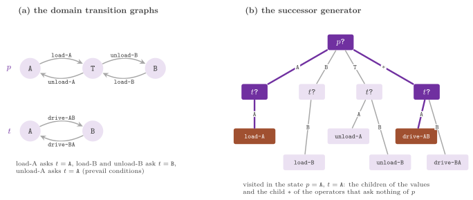
Figure 16.1 shows the generator of a small task, which we use
throughout the chapter: a package \(p\) and a truck \(t\), with the variables
\(p \in \{\mathtt{A}, \mathtt{B}, \mathtt{T}\}\) (the package at A, at B, or in
the truck) and \(t \in \{\mathtt{A}, \mathtt{B}\}\), the operators load-A,
unload-A, load-B, unload-B (each requiring the truck at its place) and
drive-AB, drive-BA, the initial state \(p = \mathtt{A}\),
\(t = \mathtt{A}\), the goal \(p = \mathtt{B}\), unit costs, and the optimal plan
load-A, drive-AB, unload-B of cost 3.
for_each_successor( s , h , f ) (Planning.h:540) visits
the generator and, for each operator \(o\) reported, computes \(t = o(s)\) and its
heuristic, and calls f( t , c(o) , h(t) ) unless \(t\) is a dead end (see
below); the form for_each_successor( s , h , op , f ) of OperatorDomain
also passes the code of \(o\) and skips the operators that undo the operator of
code op (see below). plan( path ) returns the names of the operators of a
path of states, e.g., the path of a Solution, choosing at each step the
cheapest operator that leads from a state to the next, and throws if two
consecutive states are not joined by an operator; the tests check each plan by
simulating it on the values of the variables (simulate of
test/test.h).
Dead ends¶
A heuristic of section 16.4 to 16.6 may prove that no goal is reachable from a
state, and then it returns the constant dead_end (the largest int) of
SASHeuristics.h. heuristic_or_dead( s ) returns the
value
of the heuristic of the options with dead_end, and heuristic( s ) returns 0
instead of dead_end, which keeps \(f\) within the range of the bucket queues
(Chapter 3).
Proposition 16.6 (Dead ends). A successor that the heuristic proves a dead end is not generated, and this changes no plan. Hence only the initial state can be a dead end among the states that a search handles; if it is, its value 0 is admissible, and the search expands it alone and ends without a goal.
Proof. A dead end has no path to a goal, and no plan passes through it,
and dropping it from the successors removes no plan. Every other state that a
search handles is a generated successor, hence not a dead end. A dead end \(s\)
that is the initial state has \(h(s) = 0\), admissible since \(h^*(s) = \infty\).
Its successors are dead ends for each heuristic that can return dead_end:
for those of the delete relaxation, because the facts reachable in the
relaxation from \(o(s)\) are among those reachable from \(s\) (the facts of \(o(s)\)
are those of \(s\) or added by \(o\), which is applicable in \(s\)); for the pattern
database and merge-and-shrink, because the abstract state of \(o(s)\) is reached
in the abstraction from that of \(s\) (section 16.6). Hence none of them is
generated, and the search ends after one expansion. \(\square\)
The case planning checks this on a task whose goal no operator reaches: with
\(h^{\max}\) the initial state is a dead end, heuristic returns 0, and A\(^*\)
returns unsolvable after one expansion.
The operators with an inverse¶
Lemma 16.7 (Inverse operators). Let \(o\) and \(o'\) be two operators such that (i) \(o'\) has an effect on exactly the variables of the effects of \(o\), (ii) each effect \((v, p, q)\) of \(o\) has \(p \ge 0\), and the effect of \(o'\) on \(v\) sets \(v\) to \(p\), and (iii) each precondition \(v = d\) of \(o'\) is either on a variable of an effect \((v, p, q)\) of \(o\), with \(d = q\), or a precondition of \(o\). Then, for each state \(s\) in which \(o\) is applicable, \(o'\) is applicable in \(o(s)\) and \(o'(o(s)) = s\).
Proof. Let \(t = o(s)\). A precondition \(v = d\) of \(o'\) of the first kind holds in \(t\), since \(t_v = q = d\); one of the second kind is a precondition of \(o\), which holds in \(s\), on a variable that \(o\) does not change, and hence it holds in \(t\). So \(o'\) is applicable in \(t\). It changes exactly the variables of the effects of \(o\), each to the value \(p\) that \(o\) required before, i.e., to \(s_v\); the other variables are those of \(s\). \(\square\)
The function inverse of src/Planning.cpp:230 checks
the conditions of Lemma 16.7 (with the same number of effects, each variable of
\(o\) found among those of \(o'\)), and the constructor gives the first 255
operators that have an inverse the codes \(0, \ldots, 254\) (code( o )), the
others the code no_op, with the list of the inverses of each code
(undoes( c , o ) tells whether \(o\) is an inverse of the operator of code
c). The form of for_each_successor of OperatorDomain then skips, at a
state generated by the operator of code op, its inverses, which lead back to
the parent; since the costs are not negative, this skips no cheaper path, as
§2.9 shows for the parent pruning in general. In
the task of Figure 16.1, unload-A is an inverse of load-A and drive-BA
of drive-AB. Along an optimal plan of four tasks, the case planning checks
that a state generated by a coded operator skips its parent and nothing else.
Planning passes no_op for an operator without an inverse (or beyond the
first 255), which the concept OperatorDomain allows and which only means
that nothing is skipped after it.
16.4 The delete relaxation: \(h^{\max}\), \(h^{\rm add}\) and \(h^{\rm FF}\)¶
The delete relaxation of a task ignores the delete lists of its STRIPS view: a relaxed state is a set of propositions that only grows, and a relaxed plan from \(s\) is a sequence of operators, each with its preconditions in the facts of \(s\) or added before, whose additions cover the goal. Since a plan is a relaxed plan (by Lemma 16.3, the facts of the states of a plan are among those of the relaxed states), the cost \(h^+(s)\) of an optimal relaxed plan is an admissible heuristic; it is NP-hard to compute, and the heuristics of this section approximate it.
Definition 16.8 (The heuristics of the relaxation). For a state \(s\), let \(h_s(q) = 0\) for the facts \(q \in F(s)\) and, for the other facts, $\(h_s(q) = \min_{o : q \in \mathrm{add}(o)} \Bigl( c(o) + \bigoplus_{r \in \mathrm{pre}(o)} h_s(r) \Bigr),\)$ the minimum of the empty set being \(\infty\) and \(\bigoplus\) being the maximum for \(h^{\max}\) and the sum for \(h^{\rm add}\) (the empty aggregate being 0); then \(h^{\max}(s) = \max_{g \in G} h_s(g)\) and \(h^{\rm add}(s) = \sum_{g \in G} h_s(g)\), both \(\infty\) (a dead end) if a goal fact has \(h_s(g) = \infty\). For \(h^{\rm FF}\), each fact \(q \notin F(s)\) of finite \(h_s(q)\) under \(h^{\rm add}\) has a best supporter, the operator that attains the minimum; the relaxed plan is traced back from the goal facts through the best supporters and their preconditions, and \(h^{\rm FF}(s)\) is the sum of the costs of its operators, each counted once.
In the library, the class RelaxedHeuristic computes the three:
/// the heuristic of the relaxation
enum class Kind {
 hmax ,     ///< the maximum over the preconditions
 hadd ,     ///< the sum over the preconditions
 hff        ///< the cost of the relaxed plan of h^add
 };

/// constructor, on the STRIPS view of a task, which must outlive it

RelaxedHeuristic( const StripsTask & task , Kind kind );

/// the value on the state of the values s, one per variable

[[nodiscard]] int operator()( const std::vector< int > & s ) const;
Its constructor splits each operator into its unary operators
\(\mathrm{pre}(o) \to q\), one for each \(q \in \mathrm{add}(o)\), and indexes them
by their preconditions; operator()( s )
(src/SASHeuristics.cpp:87) evaluates the values s,
one per variable, by the generalized Dijkstra algorithm of Bonet and Geffner
[135], which the following procedure transcribes
(the header has no pseudocode of it).
Algorithm 16.2 (The heuristics of the relaxation).
 1  procedure RELAXED(s)
 2     h(q) ← ∞ and best(q) ← nil for each fact q
 3     for each q ∈ F(s) do h(q) ← 0;  push (0, q)
 4     for each unary operator u: ∅ → q do relax q to c(u) by u
 5     for each unary operator u do left(u) ← |pre(u)|;  agg(u) ← 0
 6     while a goal fact is unsettled and the queue is not empty do
 7        (k, q) ← the pair of least k, removed;  if q is settled then continue
 8        settle q
 9        for each unary operator u with q ∈ pre(u) do
10           agg(u) ← agg(u) + k   (h^add, h^FF)   or   max(agg(u), k)   (h^max)
11           left(u) ← left(u) − 1
12           if left(u) = 0 then relax eff(u) to agg(u) + c(u) by u
13     if h(g) = ∞ for a goal fact g then return dead_end
14     if h^max then return max over g ∈ G of h(g)
15     if h^add then return Σ over g ∈ G of h(g)
16     trace back from G through best(·) and the preconditions, each operator once
17     return the sum of the costs of the operators traced
where "relax \(q\) to \(k\) by \(u\)" sets \(h(q) \leftarrow k\) and
\(\mathrm{best}(q) \leftarrow u\) and pushes \((k, q)\) if \(k < h(q)\). Line 6 stops
as soon as all the goal facts are settled, which is correct since the values
of the settled facts do not change afterwards. All the vectors of the
computation are
thread_local, and several workers may evaluate the heuristic at once.
Theorem 16.9 (\(h^{\max}\) is admissible and consistent). Algorithm 16.2 computes the values \(h_s\) of Definition 16.8, and for each state \(s\) and each operator \(o\) applicable in \(s\),
with \(h^{\max}(s) = 0\) if \(s\) satisfies the goal.
Proof. The aggregation (maximum or sum of nonnegative values) is monotone and not smaller than each of its arguments, and the costs are nonnegative, so that the generalized Dijkstra algorithm settles the facts in the order of their values and computes the least fixpoint of the equations of Definition 16.8, as Dijkstra's algorithm does for a sum of one argument [135]. For the admissibility, let \(\pi = o_1, \ldots, o_k\) be a relaxed plan from \(s\), \(C_i\) the cost of its prefix \(o_1, \ldots, o_i\), and \(C_0 = 0\). We show by induction on \(i\) that each fact \(q\) added by \(o_i\) has \(h_s(q) \le C_i\), and that each fact of \(s\) has \(h_s(q) = 0 = C_0\): the preconditions of \(o_i\) are facts of \(s\) or added by some \(o_j\) with \(j < i\), whence \(h_s(r) \le C_{i-1}\) for each of them, and \(h_s(q) \le c(o_i) + \max_r h_s(r) \le c(o_i) + C_{i-1} = C_i\). A plan is a relaxed plan, and its goal facts are facts of \(s\) or added by some operator of it, whence \(h^{\max}(s) \le C_k\), the cost of the plan. For the consistency, let \(t = o(s)\), and let us show \(h_s(q) \le c(o) + h_t(q)\) for each fact \(q\), by induction on the order in which the algorithm settles the facts in \(t\). If \(q \in F(t)\), either \(q \in F(s)\) and \(h_s(q) = 0\), or \(q \in \mathrm{add}(o)\) and \(h_s(q) \le c(o) + \max_{r \in \mathrm{pre}(o)} h_s(r) = c(o)\), since the preconditions of \(o\) hold in \(s\). Otherwise \(h_t(q) = c(o') + \max_r h_t(r)\) for an operator \(o'\) whose preconditions \(r\) are settled before \(q\), and $\(h_s(q) \le c(o') + \max_r h_s(r) \le c(o') + \max_r (c(o) + h_t(r)) = c(o) + h_t(q).\)$ Taking the maximum over the goal facts gives the consistency, and the value at a goal state is the maximum of zeros. \(\square\)
Proposition 16.10 (The inadmissible heuristics). \(h^{\rm add}\), \(h^{\rm FF}\) and the count of the unsatisfied goal facts are not admissible.
Proof. Let the goal be \(\{g_1, g_2\}\) and the state \(s\) hold neither. If a single operator of cost 1 adds both, the optimal cost is 1 while \(h^{\rm add}(s) = 2\) and the goal count is 2. For \(h^{\rm FF}\), let the operators be \(o_1\), adding both of cost 3, and \(o_2\) and \(o_3\), adding \(g_1\) and \(g_2\) respectively, of cost 2 each, all without preconditions: the best supporters of \(g_1\) and \(g_2\) are \(o_2\) and \(o_3\), and \(h^{\rm FF}(s) = 4 > 3 = h^*(s)\). \(\square\)
It is worth noting that \(h^{\rm FF}\) is the cost of a relaxed plan, and hence
at least \(h^+(s)\), but the plan traced is not an optimal relaxed one. The three
inadmissible heuristics serve the bounded-suboptimal searches of Chapter
6 and the greedy searches of
§2.12; on the tasks of the
data, the case planning checks that A\(^*\) with each of them returns a valid
plan, not cheaper than the optimum.
16.5 The landmark-cut heuristic¶
A disjunctive action landmark of a state \(s\) is a set \(L\) of operators such
that every plan from \(s\) contains an operator of \(L\). The landmark-cut
heuristic (LM-cut) of Helmert and Domshlak [136]
finds landmarks one after the other in the delete relaxation, and lowers the
costs in such a way that their contributions add up admissibly. In the library
it is the
class LMCut:
/// constructor, on the STRIPS view of a task, which must outlive it

explicit LMCut( const StripsTask & task );

/// the value on the state of the values s, one per variable

[[nodiscard]] int operator()( const std::vector< int > & s ) const;
Its constructor adds to the STRIPS view a fact \(\top\) that always holds, given
as a precondition to the operators that have none, and a fact \(G^\star\) added
by
a goal operator of cost 0 whose preconditions are the goal facts; thus the
goal is the single fact \(G^\star\) and each operator has a precondition. Each
evaluation (src/SASHeuristics.cpp:201) runs the
following rounds, which the header describes and the procedure transcribes, on
a copy \(c'\) of the costs.
Algorithm 16.3 (LM-cut).
 1  procedure LMCUT(s)
 2     c'(o) ← c(o) for each operator o;  h ← 0
 3     loop
 4        compute h^max(q) for each fact q from F(s) ∪ {TOP}, with the costs c'
 5        if h^max(G*) = ∞ then return dead_end
 6        if h^max(G*) = 0 then return h
 7        pcf(o) ← a precondition of o of largest h^max, for each o reached
 8        N* ← the goal zone: the facts from which G* is reached backwards by the arcs
               pcf(o) → q, q ∈ add(o), of the operators with c'(o) = 0
 9        N₀ ← the facts reached from F(s) ∪ {TOP} by the arcs pcf(o) → q
               with q ∉ N*
10        L ← the operators o with pcf(o) ∈ N₀ that add a fact of N*  ▷ the cut
11        m ← min over o ∈ L of c'(o);  h ← h + m
12        c'(o) ← c'(o) − m for each o ∈ L
In the pseudocode, TOP stands for \(\top\), N₀ for \(N^0\) and N* for
\(N^*\). The arcs \(\mathrm{pcf}(o) \to q\) form the justification graph: each
operator is reduced to its most costly precondition (the code takes the first
of the largest ones, in the order of the sorted preconditions), and \(h^{\max}\)
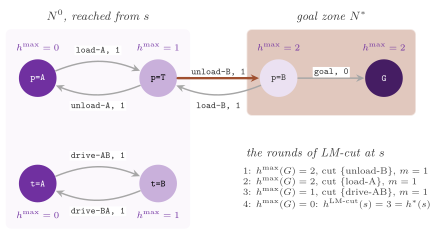
of a fact is then the cost of a shortest path in that graph. Figure
16.2 shows the first round on the task of Figure 16.1.
Lemma 16.11 (The cut is a landmark). In a round with \(0 < h^{\max}(G^\star) < \infty\), every relaxed plan from \(s\), and hence every plan, contains an operator of \(L\), and \(m > 0\).
Proof. The facts of \(F(s) \cup \{\top\}\) have \(h^{\max} = 0\); if one of them were in \(N^*\), the arcs of cost 0 from it to \(G^\star\), each from the most costly precondition of its operator, would give \(h^{\max}(G^\star) = 0\). Hence \(F(s) \cup \{\top\} \subseteq N^0\). Let \(\pi\) be a relaxed plan from \(s\) (with the goal operator at its end), and let \(o\) be its first operator that adds a fact of \(N^*\), which exists since \(G^\star \in N^*\). We show that each fact reached by \(\pi\) before \(o\) is in \(N^0\): by induction, an operator \(o'\) of \(\pi\) before \(o\) has its preconditions among the facts reached before it, which are in \(N^0\), in particular \(\mathrm{pcf}(o')\); its added facts are not in \(N^*\) by the choice of \(o\), and they are reached from \(\mathrm{pcf}(o')\) by an arc of the justification graph, whence they are in \(N^0\). Then \(\mathrm{pcf}(o) \in N^0\), and \(o\) adds a fact of \(N^*\), i.e., \(o \in L\). Finally, an operator \(o \in L\) with \(c'(o) = 0\) would put \(\mathrm{pcf}(o)\) in \(N^*\) by line 8, whereas \(\mathrm{pcf}(o) \in N^0\) and \(N^0 \cap N^* = \emptyset\); hence \(m > 0\). \(\square\)
The code throws std::logic_error if a cut is empty or has \(m \le 0\)
(src/SASHeuristics.cpp:307), which Lemma 16.11
excludes.
Theorem 16.12 (LM-cut is admissible). LM-cut ends
after finitely many rounds with integer costs, and its value is at most
\(h^*(s)\); it returns dead_end only if \(s\) is a dead end of the relaxation,
and hence of the task.
Proof. Each round lowers by \(m \ge 1\) the costs of the operators of a
nonempty cut and keeps them nonnegative, whence the sum of the costs decreases
by at least 1, and there are finitely many rounds. Let \(L_1, \ldots, L_r\) be
the cuts and \(m_1, \ldots, m_r\) their values, and let \(\pi\) be a plan from
\(s\). In the round \(i\), \(L_i\) is a landmark by Lemma 16.11, and \(\pi\)
contains an operator of \(L_i\). The final costs \(c'\) are nonnegative and
\(c(o) = c'(o) + \sum_{i : o \in L_i} m_i\); hence
$\(c(\pi) = \sum_{o \in \pi} c(o) \ge \sum_{o \in \pi} \sum_{i : o \in L_i} m_i
\ge \sum_{i=1}^{r} m_i = h,\)$
since each \(L_i\) meets \(\pi\) (an operator repeated in \(\pi\) is counted as many
times, which only adds). Finally, dead_end is returned when
\(h^{\max}(G^\star) = \infty\) in the first round, i.e., when the goal is not
reachable in the relaxation, which a plan would contradict. \(\square\)
Helmert and Domshlak also prove that LM-cut dominates \(h^{\max}\)
([136]; we have not reproduced the proof), and the
case planning checks \(h^{\max} \le\) LM-cut along an optimal plan of four
tasks. We do not claim that LM-cut is consistent; A\(^*\) remains optimal with
it, since it reopens a closed state reached by a cheaper path
(§2.7). Each round costs a computation of
\(h^{\max}\), i.e., a Dijkstra search over the facts in
\(O((|F| + U) \log |F|)\) time for \(|F|\) facts and \(U\) arcs of the operators.
The number of the rounds is usually small, but we know no bound on it better
than the sum of the costs.
16.6 Abstraction heuristics¶
An abstraction of a task maps its states onto the states of a smaller transition system in a way that preserves the paths; the distances in the abstract system are then an admissible and consistent heuristic (Chapter 5 gives the pattern databases of the permutation puzzles, built on the same principle).
Definition 16.13 (Abstraction). An abstraction is a map \(\alpha\) from the states of the task to the states of a transition system \(\mathcal{T}\), with transitions labelled by the operators and abstract goal states, such that (i) for each state \(s\) and operator \(o\) applicable in \(s\), either \(\alpha(o(s)) = \alpha(s)\) or \(\mathcal{T}\) has a transition \((\alpha(s), o, \alpha(o(s)))\), of cost \(c(o)\), and (ii) \(\alpha\) maps the goal states to abstract goal states. The heuristic of \(\alpha\) is \(h^\alpha(s) = d_{\mathcal{T}}(\alpha(s))\), the distance in \(\mathcal{T}\) from \(\alpha(s)\) to an abstract goal state.
Lemma 16.14 (Abstraction heuristics). The heuristic of an abstraction is admissible and consistent, and it is \(\infty\) only on dead ends.
Proof. By (i), a path from \(s\) to a goal of cost \(C\) is mapped onto an abstract path from \(\alpha(s)\) of cost at most \(C\) (the self-loops dropped), which ends at an abstract goal by (ii); whence \(h^\alpha(s) \le h^*(s)\), and \(h^\alpha(s) = \infty\) implies that \(s\) has no path to a goal. For an operator \(o\) applicable in \(s\), either \(\alpha(o(s)) = \alpha(s)\) and the two values are equal, or the transition of (i) gives \(d_{\mathcal{T}}(\alpha(s)) \le c(o) + d_{\mathcal{T}}(\alpha(o(s)))\). \(\square\)
Pattern databases¶
The projection onto a set \(P\) of variables (the pattern) maps a state onto
its values on \(P\), and the abstract system has the partial states on \(P\), the
transitions of the operators restricted to \(P\), and the goal restricted to \(P\);
it satisfies Definition 16.13. The class SASPatternDatabase
(src/SASHeuristics.cpp:319) stores the distances of
all its abstract states:
 /// constructor, building the distances of the projection of task onto
 /// the given variables

 SASPatternDatabase( const SASTask & task , std::vector< int > pattern );

/*- - - - - - - - - - - - - - - - - - - - - - - - - - - - - - - - - - - - -*/
 /// a pattern of at most max_size abstract states
 /** The goal variables are added while the size allows, then, in the
  * order of their indices, the variables of the preconditions of the
  * operators that change a variable of the pattern (its parents in the
  * causal graph), as long as one of them fits. */

 [[nodiscard]] static std::vector< int > greedy_pattern(
                               const SASTask & task , std::size_t max_size );
The constructor sorts the pattern, numbers the abstract state of the values \(s\)
by \(\sum_{v \in P} s_v m_v\), \(m_v\) being the product of the ranges of the
variables of \(P\) before \(v\) (the order of the sorted pattern), and throws
std::invalid_argument if a variable is out of range or if the abstract space
exceeds \(2^{40}\) states. It keeps the operators that change a variable of \(P\),
restricted to \(P\), and runs Dijkstra's algorithm backward from all the abstract
goal states: an abstract operator is regressed through a state \(j\) if \(j\) has
the values of its effects, the predecessor having the values required before by
its preconditions on \(P\) (a prevail condition must hold in \(j\) as well) and the
other values of \(j\), each variable of an effect with no value before taking
every value. Abstract states that reach no abstract goal keep the distance
dead_end. operator()( s ) looks the distance up in \(O(|P|)\),
pattern() returns the pattern and size() the number of the abstract states.
greedy_pattern( task , max_size )
(src/SASHeuristics.cpp:453) chooses the pattern when
the options give none: it adds the goal variables, in the order of the goal,
while the product of the ranges stays within max_size; then, repeatedly, it
adds the first variable, in the order of the indices, that is a parent of a
variable of the pattern in the causal graph (a variable of a precondition of an
operator that changes a variable of the pattern) and fits, until none fits.
Of course, the pattern may be empty if no goal variable fits, and then the
database has a
single abstract state of distance 0, i.e., it is the blind heuristic.
Proposition 16.15 (The pattern database). The
distances of SASPatternDatabase are those of the projection, and the
heuristic is admissible and consistent; it is built in time
\(O(N \log N \cdot |O| (|P| + R))\), \(N\) being the number of the abstract states
and \(R\) the largest number of the abstract states that the regression of an
operator through a state yields.
Proof. The regression enumerates, for an abstract state \(j\) and an abstract operator \(o\) whose effects \(j\) shows, exactly the abstract states \(i\) in which \(o\) is applicable and from which it leads to \(j\); hence Dijkstra's algorithm backward from the goals computes the distances of the projection, and Lemma 16.14 applies. Each state settled scans the \(|O|\) operators, each in \(O(|P|)\) for the test and \(O(R)\) for the predecessors, each relaxed in \(O(\log N)\) by the binary heap. \(\square\)
Merge-and-shrink¶
The class SASMergeAndShrink
(src/SASHeuristics.cpp:667) builds an abstraction
that is not a projection, by the method of Helmert, Haslum, Hoffmann and Nissim
[140]:
/// constructor, building the abstraction of the task, of at most
/// max_states states

SASMergeAndShrink( const SASTask & task , std::size_t max_states );
The atomic system of a variable \(v\) has the values of \(v\) as states, a transition \((d, o, q)\) for each effect \((v, p, q)\) of \(o\) and each \(d\) with \(p = -1\) or \(d = p\), a self-loop on \(d\) for an operator with the prevail condition \(v = d\) and no effect on \(v\), and self-loops everywhere for the operators that do not mention \(v\) (which the code marks irrelevant rather than storing them); its goal states are the value of \(v\) in the goal, or all of them. The synchronized product of two systems has the pairs of their states, a transition labelled \(o\) from \((a, d)\) to \((b, q)\) if both have a transition labelled \(o\) from \(a\) to \(b\) and from \(d\) to \(q\), and the pairs of goal states as goals. The constructor does the following.
- It takes the variables that are ancestors of the goal in the causal graph (in which \(u\) is a parent of \(v\) if an operator with an effect on \(v\) has a precondition or another effect on \(u\)), and orders them for a linear merge: the first goal variable, then repeatedly the variable of least index that is a parent of one already taken, or else the next goal variable not taken. All the other variables are left out, which is a further abstraction.
- For each variable \(v\) of the order, it shrinks the current system to at most
\(\lfloor N / |D_v| \rfloor\) states if it has more (\(N\) being
max_states, clamped to \([1, 2^{24}]\)), multiplies it by the atomic system of \(v\), so that the product has at most \(N\) states, and prunes from the product the states not reachable from its initial state and those that reach no goal state (the latter are dead ends). - The map of a state to its abstract state is kept as one table per step,
from the pair (abstract state so far, value of the variable merged) to the
abstract state after the step (\(-1\) for a pruned one), each table is
renamed when the next shrink merges states;
operator()( s )follows the tables in \(O(k)\) for \(k\) variables merged and returns the distance of the final abstract state, ordead_endif a table gives \(-1\).
variables() returns the variables in the order of the merge and size() the
number of the final abstract states. The shrink is the greedy bisimulation of
Nissim, Hoffmann and Helmert [168]
(shrink_map of src/SASHeuristics.cpp:610): it
starts from the partition of the states by their distance \(h\) to the goal (the
largest values merged into one block if there are more of them than the bound
allows), and refines it by the signatures of the states, i.e., by the pairs
(label, block of the target) of their transitions \((a, o, b)\) with
\(h(a) = c(o) + h(b)\), as long as the number of the blocks stays within the
bound; the refinement stops at the last partition within the bound, or at a
fixpoint, which is then a greedy bisimulation.
Lemma 16.16 (Shrinking by equal distances). Let a partition of the states of a system \(\mathcal{T}\), all of which reach a goal, have blocks of states of equal distance \(h\), and let \(\mathcal{T}'\) be the quotient system (a transition between two blocks for each transition between their states, and a block is a goal if it holds a goal state). Then the distance of a block in \(\mathcal{T}'\) is the common distance of its states in \(\mathcal{T}\). If the blocks of the largest distances are merged, the distance of the merged block is at most the least distance of its states.
Proof. The quotient map is an abstraction of \(\mathcal{T}\) in the sense of Definition 16.13, and the distance of a block is at most the distance of each of its states (Lemma 16.14). Conversely, a transition \((B, o, B')\) of \(\mathcal{T}'\) comes from a transition \((a, o, b)\) with \(a \in B\), \(b \in B'\), and \(h(a) \le c(o) + h(b)\); since \(h\) is constant on the blocks, \(h(B) \le c(o) + h(B')\), and along a path of \(\mathcal{T}'\) to a goal block (where \(h = 0\), a goal state having distance 0 and the block holding states of equal distance) these inequalities sum to \(h(B) \le\) the cost of the path. For the last statement, the first half of the argument suffices. \(\square\)
Hence any shrink of the library keeps the distances of the current system exact when the number of the distinct distances is within the bound, and the role of the greedy bisimulation, as Nissim et al. show [168], is to keep the information that the later products need; when it stops before its fixpoint, the abstraction is coarser, and the heuristic remains admissible.
Theorem 16.17 (Merge-and-shrink). On the states
reachable from the initial state, the heuristic of SASMergeAndShrink is
admissible and consistent, and it returns dead_end only on dead ends.
Proof. The synchronized product of the atomic systems of a set of variables
is the projection onto them (an operator applies to a pair of values exactly
when it applies to each, the task having no conditional effects), and each
shrink and each pruning is the composition with a map that merges or drops
abstract states; the composition of the tables is the map \(\alpha\) of the final
system. Merging preserves (i) and (ii) of Definition 16.13. Dropping a state
not reachable from the abstract initial state affects no state reachable from
the initial state of the task, since by (i) such a state is mapped onto an
abstract state reachable from the abstract initial state; dropping a state that
reaches no abstract goal maps the states onto it to dead_end, which is
correct, since a concrete path to a goal would be mapped onto an abstract one.
Hence, on the reachable states, \(\alpha\) is an abstraction of the task into the
final system, and Lemma 16.14 applies. \(\square\)
Cartesian abstractions refined by counterexamples¶
The class SASCartesianAbstraction
(src/SASHeuristics.cpp:1173) builds an abstraction
by counterexample-guided abstraction refinement (CEGAR), the method of Seipp
and Helmert [200],
[201]. Instead of fixing a set of variables in
advance, as a projection does, it starts from the coarsest abstraction and
splits only the abstract states on which an optimal abstract plan fails in the
task (the counterexamples).
/// the limits of the refinement
struct Limits {
 std::size_t max_states = 1000;           ///< the most abstract states
 std::size_t max_transitions = 1000000;   ///< the most transitions
 double max_time = 0;                     ///< the seconds, 0 for no limit
 };

/// constructor, refining the abstraction of the task within the limits

explicit SASCartesianAbstraction( const SASTask & task ,
                                  const Limits & limits );

/// constructor, refining the abstraction of the subtask of task with the
/// given goal and costs, one per operator, within the limits

SASCartesianAbstraction( const SASTask & task ,
                         std::span< const SASTask::Fact > goal ,
                         std::span< const int > cost ,
                         const Limits & limits );
An abstract state is a Cartesian set \(a = A_0 \times \cdots \times A_{n-1}\), with \(\emptyset \neq A_v \subseteq D_v\), and the abstract states partition the states of the task. The system has a transition \((a, o, b)\), \(b \neq a\), if \(o\) leads from a state of \(a\) to a state of \(b\), and \(a\) is an abstract goal if it holds a state that satisfies the goal; since \(a\) and \(b\) are products, both conditions are tested variable by variable. For an operator \(o\) and a variable \(v\), let \(\mathrm{pre}_v(o)\) be the value that \(o\) asks of \(v\) (by a prevail condition or by an effect with a value before), if any, and \(\mathrm{post}_v(o)\) the value that it gives \(v\), if any.
Lemma 16.18 (Cartesian abstractions). Let \(a\) and \(b\)
be Cartesian sets. Then \(o\) leads from a state of \(a\) to a state of \(b\) if and
only if, for each variable \(v\), (i) \(\mathrm{pre}_v(o) \in A_v\) when it is
defined, and (ii) \(\mathrm{post}_v(o) \in B_v\) when it is defined, or else
\(\mathrm{pre}_v(o) \in B_v\) when \(\mathrm{pre}_v(o)\) is defined, or else \(A_v
\cap B_v \neq \emptyset\). Hence the system of Cartesian sets with these
transitions satisfies Definition 16.13, its heuristic is admissible and
consistent on every state, and it is dead_end only on dead ends.
Proof. The conditions are necessary: a state \(s \in a\) in which \(o\) applies has \(s_v = \mathrm{pre}_v(o)\), and \(o(s)_v\) is \(\mathrm{post}_v(o)\), or \(s_v\) if \(o\) does not change \(v\). They are sufficient, since a product lets one choose \(s_v\) for each variable apart: \(s_v = \mathrm{pre}_v(o)\) where it is defined, a value of \(A_v \cap B_v\) for a variable that \(o\) neither mentions nor changes, and any value of \(A_v\) otherwise; the task having no conditional effects, \(o\) applies in \(s\) and \(o(s) \in b\). Hence (i) of Definition 16.13 holds, with the self-loops dropped, and (ii) holds by the definition of the abstract goals. Hence Lemma 16.14 applies, and it applies to all the states, since no abstract state is pruned. \(\square\)
Each abstract state remembers its incoming and outgoing transitions and its self-loops, labelled by the operators, and the refinement proceeds as follows.
Algorithm 16.4 (CEGAR).
 1  procedure CEGAR(task, goal G, costs c)
 2     the single abstract state of all the states, every operator a self-loop
 3     while no limit is reached
 4        a₀ ← the abstract state of s₀;  π ← an optimal abstract plan from a₀
 5        if there is no such plan then leave the loop   ▷ s₀ is a dead end
 6        s ← s₀;  a ← a₀
 7        for each step (o, b) of π
 8           if o does not apply in s then
 9              split a by {p} on a v with pre_v(o) = p ≠ s_v;  continue at 3
10           if o(s) ∉ b then
11              split a by A_v ∩ B_v on a v with o(s)_v ∉ B_v;  continue at 3
12           s ← o(s);  a ← b
13        if s misses a fact v = g of G then
14           split a by {g} on v;  continue at 3
15        leave the loop                                 ▷ π is a plan of the task
16     the goal distances h, by Dijkstra's algorithm backward from the goals
In the pseudocode, "split \(a\) by \(W\) on \(v\)" replaces \(a\) by the two Cartesian sets whose sets of values of \(v\) are \(A_v \setminus W\) and \(A_v \cap W\), and whose other components are those of \(a\). Each split is proper, i.e., both parts are nonempty: at line 9, \(p \in A_v\) (the transition of \(\pi\) out of \(a\) exists, whence (i) of Lemma 16.18) and \(s_v \in A_v \setminus \{p\}\); at line 11, \(o\) does not change \(v\) (otherwise \(o(s)_v = \mathrm{post}_v(o) \in B_v\) by (ii)), and hence \(s_v = o(s)_v \notin B_v\), while \(A_v \cap B_v \neq \emptyset\) by (ii); at line 14, \(g \in A_v\) (\(a\) is an abstract goal) and \(s_v \neq g\). Since the state \(s\) of the trace stays in the abstract state \(a\) of the plan (the test of line 10), the split separates \(s\) from the part of \(a\) whose states admit the step of the plan that failed. When several variables offer a flaw of the same kind, the code splits on the one whose \(A_v\) is the smallest fraction of \(D_v\), the least index on a tie (the most refined one, one of the strategies compared in [201]).
The engineering is the following. A split rewires only the transitions of the
abstract state split: each incoming transition, outgoing transition and
self-loop of \(a\) is tested, by the condition of Lemma 16.18 on the variable \(v\)
alone (the other components did not change), against the two parts; since a
transition out of (or into) a part is also one of \(a\), the transitions after
the split are those of the new system (cf. Lemma 16.18). The optimal abstract
plan of line 4 is found by A\(^*\) with the goal distances of an earlier
abstraction as heuristic, the new part of a split taking the distance of the
state split. Indeed, a split may only remove transitions and abstract goals,
and therefore these distances remain admissible and consistent; they are
computed again whenever the number of the abstract states has grown by a
quarter. In turn, the map of a state to its abstract state is the refinement
hierarchy, a binary tree whose leaves are the abstract states and whose inner
nodes are the splits, each testing whether the value of its variable is among
those of \(W\); operator()( s ) descends it in \(O(k)\) steps for a leaf of depth
\(k\) and returns the distance of the leaf. Finally, the Limits bound the
abstract states (1000 by default), the transitions (\(10^6\)) and the seconds of
the refinement (none by default), and are tested before each split (hence a
limit on the transitions may be exceeded by the transitions of the last split).
size() and transitions() return the numbers of the abstract states and of
the transitions, and exact_init() is true if the refinement ended at line 15.
Note that the refinement terminates, since each split adds an abstract state and there are at most \(\prod_v |D_v|\) of them. If it ends at line 15, the operators of \(\pi\) form a plan of the task of cost \(h(a_0)\), and since \(h(a_0) \le h^*(s_0)\) by Lemma 16.18, the value of the initial state is its optimal cost; if it ends at line 5, the initial state is a dead end. Otherwise the abstraction is the one reached within the limits, and its value on the initial state may be below the optimal cost.
Additive Cartesian abstractions¶
A single abstraction of the task typically spends its abstract states on one
goal fact after another; Seipp and Helmert [202]
build instead one abstraction for each goal fact and add their values under
saturated cost partitioning. The class SASAdditiveCartesian
(src/SASHeuristics.cpp:1258) does so:
/// constructor, refining the abstractions of the goal facts of task
/// within the limits, max_states and max_time being on their total

SASAdditiveCartesian( const SASTask & task ,
                      const SASCartesianAbstraction::Limits & limits );
The second constructor of SASCartesianAbstraction refines the abstraction of
a subtask, i.e., of the task with another goal and other costs, and
saturated_costs() returns, for each operator \(o\),
the inner maximum taken over the transitions labelled \(o\) with \(h(b)\) finite
(the maximum of the empty set being \(-\infty\)). For the goal facts \(g_1,
\ldots, g_k\), in the order of the goal, SASAdditiveCartesian refines the
abstraction \(h_i\) of the subtask whose goal is \(\{g_i\}\) with the costs \(c_i\),
where \(c_1 = c\) and \(c_{i+1} = c_i - \sigma_i\), and its value is \(h(s) = \sum_i
h_i(s)\), or dead_end if one of the terms is. The limits on the abstract
states and on the time are on the total: each abstraction gets those left,
divided by the number of the abstractions left (at least one state), and the
construction stops after an abstraction in which the initial state is a dead
end.
Theorem 16.19 (Saturated cost partitioning). For each
\(i\), \(0 \le \sigma_i \le c_i\), the distances of the abstraction \(h_i\) are the
same under the costs \(\sigma_i\) as under \(c_i\), and \(\sum_i \sigma_i \le c\).
Hence the heuristic of SASAdditiveCartesian is admissible and consistent on
every state, and it is dead_end only on dead ends.
Proof. A transition \((a, o, b)\) with \(h_i(b)\) finite has \(h_i(a) \le c_i(o) +
h_i(b)\), since the distances are computed under \(c_i\); hence \(\sigma_i(o) \le
c_i(o)\), and \(c_{i+1} \ge 0\). Under \(\sigma_i\) no distance is smaller, since
\(\sigma_i \le c_i\), and none is larger: each transition \((a, o, b)\) with
\(h_i(b)\) finite has \(h_i(a) \le \sigma_i(o) + h_i(b)\) by the definition of
\(\sigma_i\), and summing these inequalities along a path to a goal gives \(h_i(a)
\le\) its cost under \(\sigma_i\). By induction, \(\sum_{j \le i} \sigma_j = c -
c_{i+1} \le c\). Now let \(s\) have a path to a goal of cost \(C\), whose operators
\(o\) cost \(c(o) \ge \sum_i \sigma_i(o)\): by Lemma 16.18 under the costs
\(\sigma_i\), \(h_i(s)\) is at most the cost of the path under \(\sigma_i\), and the
sum over \(i\) is at most \(C\). For consistency, the same argument on an operator
\(o\) applicable in \(s\) gives \(h_i(s) \le \sigma_i(o) + h_i(o(s))\) for each \(i\),
and the sum is at most \(c(o) + h(o(s))\). A term is dead_end only on a dead
end of its subtask, which is a dead end of the task, since the goal of a
subtask is a part of the goal. \(\square\)
Of course, the result depends on the order of the subtasks, the first ones taking the costs that they saturate; the code keeps the order of the goal, while Seipp and Helmert also study other orders and the subtasks of the landmarks of the task [201], which the library does not implement.
The case planning checks the optimal costs of the tasks with the pattern
database, with merge-and-shrink and with the Cartesian abstractions, the
admissibility of the first two along an optimal plan and their consistency on
each successor of the states of the plan. For the Cartesian abstractions, it
enumerates the states reachable in five small tasks and checks, against their
distances to the goal computed backward, that both heuristics are 0 on the
goals, admissible and consistent, that the additive one is not below each of
its terms, and that exact_init() implies an exact value of the initial state;
it also checks the limits on the abstract states and on the time, the dead end
of a task whose goal no operator reaches, and, on four tasks, that A\(^*\) with
each of the two heuristics finds the optimal cost and expands no more states
than with \(h^{\max}\).
16.7 Features and abstractions for the parallel searches¶
The distributions of HDA\(^*\) and the nblocks of PBNF need the structure of the
task, which PlanningBase derives from it as follows.
The features of Zobrist hashing¶
The features of a state are its facts, i.e., the propositions of the STRIPS
view (num_features() is their number, and for_each_feature( s , f ) calls
f for the fact of each variable), as in the HDA\(^*\) for planning of
Kishimoto, Fukunaga and Botea [2]. A move changes
the facts of the variables that its operator sets, and
for_each_feature_change( s , t , f ) (Planning.h:606)
finds them by the exclusive or of the words of the two states and the fields of
the variables of each word that differs; the incremental Zobrist key
of §9.5 costs \(O(W + e)\) for \(e\) variables
changed. In the case planning, we check that the facts reported are the
symmetric
difference of the facts of \(s\) and \(t\) on each successor of the states of an
optimal plan.
The abstract features of FAZHDA\(^*\)¶
The abstraction of the features for Abstract Zobrist hashing is that of
FAZHDA\(^*\) of Jinnai and Fukunaga ([138], section
3, and [5], section 4.2, as the header reports
them). The fluency of a variable is the number of the effects that change it
(those with \(p \ne q\), an effect with \(p = -1\) counting as a change); the
fraction ignored of the variables of largest fluency (the first
\(\lfloor \mathit{ignored} \cdot n \rfloor\) in the order of decreasing fluency,
ties by index) is left out, and all their facts are mapped to the abstract
feature 0, whose key is the same in all the states; their moves never
change the owner of a state. The values of each other variable are split into
two abstract features by GreedyAFG: on the undirected domain transition graph
of
the variable (an edge \(\{d, q\}\) for each effect that may change \(d\) into \(q\)),
the first half \(S_1\) starts from a value of least degree and grows by the value
with the most edges into \(S_1\) (the first one on a tie) until it holds
\(\lceil |D_v| / 2 \rceil\) values; the facts of \(S_1\) and of the rest get two
abstract features of their own. A move of such a variable then changes the
owner only if it crosses from one half to the other, and the halves are chosen
to keep most transitions inside one half. With ignored \(= 0\) the abstraction
is that of GAZHDA\(^*\). num_abstract_features() and abstract_feature( i )
give the abstraction to AbstractZobristDistribution; the case planning
checks that each abstract feature is in range.
The groups and the transitions¶
The automatic distributions of Chapter 10
read two further structures of the task. The groups of the features are the
variables (num_feature_groups() is \(n\) and feature_group( i ) the variable
of the fact \(i\)), whose facts are mutually exclusive, as the concept
FeatureGroupDomain requires. The transitions are the arcs of the domain
transition graphs: for_each_feature_transition( f )
(Planning.h:269) calls f( i , j ) for each operator, each
effect \((v, p, q)\) and each fact \(i\) of \(v\) that the effect may delete (\(v =
p\),
or every \(v = d\) with \(d \ne q\) if \(p = -1\)) and the fact \(j\) (\(v = q\)) that it
adds; each arc is reported once per operator that realizes it, which gives
the weights of the cuts of GRAZHDA\(^*\). In the case planning, we check that
both facts of each arc are of the same variable and that each move of the
states of
an optimal plan is an arc reported. How the distributions use them is the
subject of Chapter 10.
The nblocks and the abstract states¶
The nblocks of Safe PBNF, which are also the abstract states of AHDA\(^*\)
(abstract_state( s ) returns nblock( s )), are the states of the projection
onto a set of variables chosen by the greedy abstraction of structured
duplicate detection of Zhou and Hansen [139]
(described also in section 2.4 of [3]).
PlanningBase::build_nblocks (src/Planning.cpp:511)
starts from the empty set of variables and adds one at each step. The
candidates are the variables \(v\) not yet taken with \(|D_v| \ge 2\) such that the
projection onto the set with \(v\) has at most max_nblocks states and, if
nblock_facts is positive, the variables of the set hold at most that
fraction of the facts (the dynamic threshold of DAHDA\(^*\), section 5 of
[138] as the header reports it). For each
candidate the code builds the directed abstract graph of the projection (an
edge from each abstract state matching the preconditions of an operator that
changes a variable of the set to the abstract state after its effects), and
it takes the variable whose graph has the least largest out-degree, the larger
graph on a tie; it stops when no variable fits. The graph of the
final set is then made undirected, its edges taken in both directions, and
stored in compressed rows: num_nblocks() is the number of its nodes,
nblock_vars() the variables of the projection, nblock( s ) the index of the
projection of \(s\) in mixed radix, and for_each_nblock_successor( b , f )
calls f for the neighbours of \(b\). This abstraction is built at its first
use,
under a std::once_flag: a search that needs no nblocks does not pay
for it, and several workers may require for it at once.
Proposition 16.20 (The nblocks are an
abstraction). The projection chosen by build_nblocks, with its undirected
graph, satisfies the conditions (i) and (ii) of Definition
11.1. Building it takes
\(O(n \cdot |O| \cdot N \cdot (k + e) \cdot \log_2 N)\) time, \(N\) being
max_nblocks, \(k\) the number of the variables of the projection and \(e\) the
largest number of effects of an operator.
Proof. (i) Let \(o\) be applicable in \(s\). If \(o\) changes no variable of the
projection, \(s\) and \(o(s)\) have the same nblock. Otherwise the abstract state
of \(s\) matches the preconditions of \(o\) on the variables of the projection, so
that the enumeration of the abstract states matching them (the odometer of
abstract_graph) reaches it and adds the edge to the abstract state after the
effects, which is that of \(o(s)\), if the two differ. (ii) The graph is made
symmetric, and no node is its own neighbour, since an edge is added only
between two different abstract states. For the time, each step multiplies the
size of the projection by at least 2, whence there are at most \(\log_2 N\)
steps; each step tries at most \(n\) variables, and each graph enumerates, for
each of the \(|O|\) operators, at most \(N\) abstract states in \(O(k + e)\) each.
\(\square\)
The case planning checks, along an optimal plan of four tasks, that the
nblock of each successor is that of its parent or one of its neighbours, and
that the graph is undirected; the parallel cases build the nblocks with at most
512 of them, which keeps the build of the coverage within its time.
16.8 The goal test at the generation¶
On planning tasks, whose costs are often all 1 and whose heuristics are often
weak, the last layer of \(f = C^*\) may be large, and the planners test the goal
when a node is generated. The sequential A\(^*\) does so with the option
SearchOptions::goal_at_generation of Solution.h, which
§2.11 describes with its proof of optimality
(Theorem 2.21): A\(^*\) keeps the incumbent, the
goal of least \(g\) among those generated with \(h = 0\), and returns it as soon as
no entry of OPEN has a smaller \(f\), which saves the nodes of \(f = C^*\) that
come
before a goal in the order of the ties, and all of the last layer when the
parent of an optimal goal has \(f < C^*\). A successor is tested only if its \(h\)
is 0, and an informative heuristic pays little for the option; the
goals that improve the incumbent are counted in
SearchStats::goals_generated.
We check the option, in the case planning, on the tasks of the data. With the
blind
heuristic, A\(^*\) with the option expands exactly the states closer to the
initial state than the optimum (counted by a breadth-first search, the costs
being 1) on four tasks, and without it at least as many. With LM-cut, the
option saves one expansion on each of four tasks: 284 and 283 nodes on
blocks-6-2, 77 and 76 on logistics-4-0, 23 and 22 on driverlog-03, 83 and
82 on gripper-01 (with the default data structures, whose order of the ties
these counts depend on). AStarBench sets the option by --gengoal 0 | 1, by
default 1 for --domain planning and 0 otherwise; the parallel searches do not
honour it.
16.9 The searches on planning tasks¶
Since Planning models the concepts of section 16.3, every search of the
library whose concepts it models runs on a task: A\(^*\) and its variants,
IDA\(^*\), the search with delayed duplicate detection on the disk
(§4.6), the bounded-suboptimal and the greedy
searches, and the parallel ones, i.e., SPA\(^*\), MQA\(^*\) and the farm
(Chapter 8), HDA\(^*\) with the distributions Z,
AZ, A, H and R, with P for Planning< 1 >, and with the automatic
distributions of Chapter 10, Safe PBNF and
the
parallel structured duplicate detection (Chapter 11,
Chapter 12), and HDA\(^*\) over MPI
(§9.6). Searches that need a concept
that Planning does not model refuse it at compile time or, in AStarBench,
with an exception: e.g., the bidirectional searches (no predecessors), the
edge-based ones of PA\(^*\)SE (no pairwise heuristic), EPEA\(^*\) (no selection of
the operators by \(\Delta f\)), SIW (no goal features) and the hyperplanes (no
levels). The case planning runs A\(^*\) on the 28 tasks with each admissible
heuristic (but the pairs that take more than a few thousand expansions in the
unoptimized build of the coverage) and with the inadmissible ones on eight
tasks, IDA\(^*\) on three tasks and the search on the disk on four. The case
planning-thread runs HDA\(^*\) with Z, AZ, A, H and P, the farm, Safe PBNF,
SPA\(^*\) and MQA\(^*\) with 1, 2, 3 and 8 workers on four tasks, with
merge-and-shrink and at most 512 nblocks; planning-openmp and
planning-fastflow do the same on the other executors, the latter without Safe
PBNF, SPA\(^*\) and MQA\(^*\). Finally, the case mpi runs HDA\(^*\) over MPI with Z
and AZ on blocks-6-2.
AStarBench --domain planning --file <output.sas> reads a task by
SASTask::read_file and builds a Planning< 2 > if words_for gives at most
two words and a Planning< 16 > otherwise (two sizes only, since each one
instantiates every search, and the build of the coverage runs out of memory
with three; a task of more than 16 words is refused). Its options for the
domain
are --heur blind | goalcount | hmax | hadd | hff | pdb | lmcut | mas | cegar
| cegaradd (lmcut by default), --pdbsize (the most abstract states of the
greedy pattern, 65536), --massize (those of merge-and-shrink, 1000),
--cegarsize and --cegartime (those of the Cartesian abstractions, 1000, and
the seconds of their refinement, 0 for no limit), --ignored
(the fraction of the variables left out of the abstraction of AZH, 0.3),
--nblocks (the most nblocks, 10000), --nbfacts (the largest fraction of the
facts in the nblocks, 0 for no limit) and --gengoal. For instance,
AStarBench --domain planning --file data/planning/logistics-6-0.sas --heur
mas --algo hda --dist AZ --threads 8
solves the task with HDA\(^*\) on 8
workers,
the distribution of FAZHDA\(^*\) and merge-and-shrink.
16.10 The tasks of the data¶
data/planning holds 28 small tasks of the International Planning
Competitions, written by tools/pddl2sas.py from the PDDL files
of the collection of the benchmarks of Fast Downward: the domains gripper of
IPC 1998, blocks and logistics00 of IPC 2000, and driverlog of IPC 2002. Its
list optimal.txt gives the cost of an optimal plan of each
(all the costs are 1), marked by * when the lower and the upper bound of the
public collection planning.domains coincide, and in any case proved by A\(^*\)
with the blind heuristic (as the file states); the IPC tasks carry no license
nor copyright notice and are redistributed freely by the public collections of
planning benchmarks. Table 16.1 gives their sizes, which we counted on the
files.
Table 16.1. The tasks of data/planning: the number of the
variables, of the facts (the propositions of the STRIPS view), of the operators
and of the goal facts, and the optimal costs of optimal.txt.
All the states fit in one word of 64 bits.
| tasks | variables | facts | operators | goal facts | optimal costs |
|---|---|---|---|---|---|
blocks-4-0 to -2 |
9 | 34 | 32 | 3 | 6, 10, 6 |
blocks-5-0 to -2 |
11 | 47 | 50 | 4 | 12, 10, 16 |
blocks-6-0 to -2 |
13 | 62 | 72 | 5 | 12, 10, 20 |
blocks-7-0 to -2 |
15 | 79 | 98 | 6 | 20, 22, 20 |
driverlog-01 |
8 | 34 | 88 | 4 | 7 |
driverlog-02 |
9 | 41 | 108 | 7 | 19 |
driverlog-03 |
10 | 46 | 120 | 6 | 12 |
gripper-01 to -04 |
7 to 13 | 24 to 54 | 34 to 82 | 4 to 10 | 11, 17, 23, 29 |
logistics-4-0 to -2 |
9 | 48 | 78 | 4 | 20, 19, 15 |
logistics-5-0 to -2 |
9 | 48 | 78 | 5 | 27, 17, 8 |
logistics-6-0 to -2 |
9 | 48 | 78 | 6 | 25, 14, 25 |
The tasks are small on purpose: the tests solve them with each heuristic in the unoptimized build of the coverage, and the larger tasks of the same domains are translated by the same script.
16.11 The benchmark¶
We compare, first, the admissible heuristics under the sequential A\(^*\) on the
28 tasks, and, second, the parallel searches with merge-and-shrink. Our first
table gives, for each task and each of the heuristics blind, hmax, lmcut,
pdb and mas, the expansions and the seconds, with the goal test at the
generation (the default of AStarBench for planning); the expansions do not
depend on the machine, but they depend on the order of the ties of the OPEN
list.
Table 16.2. A\(^*\) with the admissible heuristics on the tasks of
data/planning: for each task, the optimal cost, and for each
heuristic the expansions and the seconds (the median of two runs); the machine
and the compiler are given in the note of the table.
| task | C* | blind | hmax | lmcut | pdb | mas |
|---|---|---|---|---|---|---|
Placeholder: the results of this table are to be measured on an idle machine and written here by manual/build/tables.py; no number is given until then.
Table 16.3. The parallel searches on the larger tasks of
data/planning with merge-and-shrink: HDA\(^*\) with the
distributions Z, AZ (FAZHDA\(^*\)) and A, and Safe PBNF, on the threads of C++
with 8 workers; for each task and search, the seconds, the speedup over
sequential A\(^*\), the search overhead SO, the communication overhead CO and the
load balance LB of §8.2.
| task | search | seconds | speedup | SO | CO | LB |
|---|---|---|---|---|---|---|
Placeholder: the results of this table are to be measured on an idle machine and written here by manual/build/tables.py; no number is given until then.
The tables are written by manual/build/tables.py from the CSV of
the campaign; until the runs are made on an idle machine, they are
placeholders that say so. The clock is the field seconds of the Solution,
which does not include the reading of the task nor the construction of the
domain (the pattern database or the merge-and-shrink abstraction, built once
by the constructor, and the nblocks, built at their first use within the
search, which the clock therefore includes for Safe PBNF and AHDA\(^*\)).
16.12 Notes and references¶
The SAS+ formalism is that of Bäckström and Nebel [133], and the format of the files, the successor generator and the causal graph are those of Fast Downward [134]. The heuristics of the delete relaxation are due to Bonet and Geffner [135] (\(h^{\max}\) and \(h^{\rm add}\)) and to Hoffmann and Nebel [101] (\(h^{\rm FF}\), in the form traced from the best supporters of \(h^{\rm add}\) of Keyder and Geffner [173]), the landmark-cut heuristic to Helmert and Domshlak [136], the pattern databases for planning to Edelkamp [137], and merge-and-shrink to Helmert, Haslum, Hoffmann and Nissim [140], with the greedy bisimulation of Nissim, Hoffmann and Helmert [168], and the Cartesian abstractions refined by counterexamples, with their additive form under saturated cost partitioning, to Seipp and Helmert [200], [201], [202]. On the parallel side, HDA\(^*\) was proposed for planning with the facts as the features of Zobrist hashing by Kishimoto, Fukunaga and Botea [2], and the abstractions of FAZHDA\(^*\), GAZHDA\(^*\) and DAHDA\(^*\) are those of Jinnai and Fukunaga [138], [141], [5]; the greedy abstraction of the nblocks is that of the structured duplicate detection of Zhou and Hansen [139]. The sections of the papers cited in this chapter are those of the comments of the headers, which we have not checked against the papers.
It is fair to remark that the library is not a planner. Its translator handles STRIPS with types only, without the action costs, the conditional effects, the quantifiers and the derived predicates of PDDL, and its invariant synthesis is a simple search over candidates of up to three predicates; its heuristics are the classical ones, in their basic forms (e.g., the linear merge and a single shrink strategy for merge-and-shrink, one greedy pattern for the pattern database, the subtasks of the goal facts alone, in the order of the goal, for the additive Cartesian abstractions), and its tasks are small. Rather, the domain serves to run the searches of the library, sequential and parallel, on a domain-independent problem whose structure is read from a file, and to compare them with the planners in the literature on the same tasks.
16.13 Exercises¶
Exercise 16.1 (ctest -R PBeFS.planning). Write the task of section 16.1
of one variable of three values with the operators ab (0 to 1, cost 5), bc
(1 to 2, cost 1) and any-c (any value to 2, cost 7) in the format
output.sas, and show that its optimal cost is 6 with each admissible
heuristic. Then show why the reader refuses a conditional effect, an axiom, a
negative cost, a value out of range and the version 2 of the format.
Exercise 16.2 (ctest -R PBeFS.planning). Compute, on the task of Figure
16.1, \(h^{\max}\), \(h^{\rm add}\), \(h^{\rm FF}\), the goal count and LM-cut at the
initial state, and verify the three rounds of LM-cut given in Figure 16.2.
Which of the values equal \(h^* = 3\)?
Exercise 16.3 (ctest -R PBeFS.planning). Prove that, with the blind
heuristic, unit costs and the goal test at the generation, A\(^*\) expands
exactly the states whose distance from the initial state is less than \(C^*\), as
the case checks by a breadth-first search (use
Theorem 2.21); why may the count of the expansions
without the option exceed it?
Exercise 16.4 (ctest -R PBeFS.planning). Show by Lemma 16.7 that, in
the task of Figure 16.1, unload-A is an inverse of load-A and drive-BA of
drive-AB, and that unload-B is not an inverse of load-A. Check that the
case finds that a state generated by a coded operator skips its parent and
nothing else.
Exercise 16.5 (ctest -R PBeFS.planning). Prove that the pattern database
of the greedy pattern of blocks-6-2 is consistent (Proposition 16.15) and
that merge-and-shrink is consistent on the reachable states (Theorem 16.17);
give a state, not reachable from the initial one, on which merge-and-shrink may
return dead_end although a goal is reachable from it.
Exercise 16.6 (ctest -R PBeFS.planning-thread). Show that, under
FAZHDA\(^*\) with ignored \(= 0.3\), the moves of the variables left out never
change the owner of a state, and that the nblocks of the case (at most 512)
satisfy Definition 11.1 (Proposition 16.20). Check
that HDA\(^*\), the farm, Safe PBNF, SPA\(^*\) and MQA\(^*\) find the optimal costs
of
the four tasks of the case with 1, 2, 3 and 8 workers.
Exercise 16.7 (ctest -R PBeFS.mpi). Explain why HDA\(^*\) over MPI can run
on a task whose states are arrays of words with the distributions Z and AZ,
which need only the facts and their abstraction, and check that the case finds
the optimal cost 20 of blocks-6-2 with both.
Exercise 16.8 (ctest -R PBeFS.planning). Run Algorithm 16.4 by hand on
the task of section 16.1 of one variable of three values (the operators ab,
bc and any-c of Exercise 16.1), and show that it ends at line 15 with
three abstract states and the value 6 of the initial state. Then show, by
Lemma 16.18, why the task whose only operator is ab gives two abstract
states and the value dead_end of its initial state, as the case checks.