13. Branch-and-bound and its parallel schemes¶
[Source: include/PBeFS/bnb/BranchAndBound.h (the concept,
the options, the solution, the queue and the sequential search),
include/PBeFS/bnb/ParallelBranchAndBound.h (the
shared incumbent, the shared and the distributed queues),
MultiQueueBranchAndBound.h,
FarmBranchAndBound.h,
DeterministicBranchAndBound.h,
StealingBranchAndBound.h,
SelfSplitBranchAndBound.h,
MPIBranchAndBound.h,
BranchAndBoundScheme.h,
SkeletonBranchAndBound.h,
RacingBranchAndBound.h,
BBCheckpoint.h,
MPIHubBranchAndBound.h,
IntervalBranchAndBound.h,
Knapsack.h, MaxClique.h,
MaxCommonSubgraph.h,
SubgraphIsomorphism.h, QAP.h,
Flowshop.h and UTS.h of the same directory;
tools/BranchAndBoundBench.cpp;
test/test.cpp, test/bb.cpp and
test/bnb.cpp]
We are concerned in this chapter with the minimization of a function \(v\) over a finite (but possibly "huge") set \(X\), i.e., with finding
when \(X\) can be partitioned recursively into smaller sets, each of which comes with a lower bound on the values that it contains; a maximization is the minimization of \(-v\), which is how the library treats it internally. The method is branch-and-bound (B&B), which Land and Doig [146] introduced for discrete programming. A\(^*\) is a special case of it [17]: the subsets are the nodes of a tree, the bound of a node plays the part of \(f = g + h\), and the best value found so far (the incumbent) prunes the nodes that cannot improve on it. The layer of the library that implements B&B shares with the graph searches of the previous chapters the executors of the workers (§1.6), their placement on the cores and the detection of the termination. It does not share the node table and the OPEN lists of A\(^*\), which are specialized for integer costs and for the duplicates of a graph.
The structure of the chapter is as follows. §13.1 gives the
concept BranchAndBound and the types around it, and §13.2
the notions of node, bound, estimate and pruning, on the 0-1 knapsack
that serves as the running example of the chapter. §13.3
gives the sequential search, §13.4 its correctness and the
bound it reports when it stops early, and §13.5 the rules
by which it selects the next node, depth-first B&B among them, together
with the queue that implements them and the cost of the whole search.
§13.6 shows A\(^*\) as a special case. §13.7
states what a parallel B&B has to guarantee, with the shared incumbent,
the dive and the limits common to all the schemes. §13.8
and §13.9 then give the eight parallel schemes of the
library, each with its pseudocode, the invariant that makes its result
optimal, the proof that its detection of the end is sound and that the
end comes, and its engineering: first those with one pool of open nodes
(the shared queue, the MultiQueue, the farm and the deterministic
rounds), then those with one pool per worker (the distributed queues,
their version over MPI, the work stealing and the SelfSplit).
§13.10 compares the schemes and shows how a program
chooses one by its name. §13.11 treats the reoptimization
from the leaves of a previous search, and §13.12 the
interface that a B&B solver built on a modeling system would use. The
next sections extend the core:
§13.13 gives the children built one at a time and the modes
that decide or enumerate instead of optimizing, §13.14 the
depth-first search skeletons, §13.15 the racing ramp-up,
§13.16 the checkpoints, §13.17 the master,
hubs and workers over MPI, §13.18 the work stealing of
intervals of leaves, and §13.19 the example problems that
exercise them (the maximum clique, the maximum common subgraph, the
subgraph isomorphism, the quadratic assignment, the permutation flowshop
and the unbalanced tree search); §13.20 to
§13.22 give the benchmark, the notes and the exercises of
the whole chapter. The
notation is that of Chapter 1, and the
conventions of the pseudocode are those of
§1.4. In the pseudocode, as in the
headers, \(\beta(n)\) is the bound of the node \(n\), \(z\) the incumbent
value, Q a queue of open nodes and \(p\) the number of workers.
13.1 The problem and its interface¶
A problem is given to the B&B layer as a type P that satisfies the
concept BranchAndBound (BranchAndBound.h:417),
i.e., that provides
- the copyable type
node_typeof its nodes; - the constant
sense,Sense::minimizeorSense::maximize; - the method
root(), which gives the node of the whole set \(X\); - optionally, the type
value_typeof its values,doubleif it gives none; - either the methods
evaluate( n )andbranch( n , sink )of aBBEvaluator(BranchAndBound.h:369), which have to be safe to call concurrently in a parallel search, or the methodmake_worker( i ), which returns theBBEvaluatorof the worker \(i\).
In the header the concept reads as follows (the concepts BBValue and
BBEvaluator are described below):
template< class P >
concept BranchAndBound = requires( const P & p , unsigned i ) {
 typename P::node_type;
 requires std::copyable< typename P::node_type >;
 requires BBValue< bb_value_t< P > >;
 { P::sense } -> std::convertible_to< Sense >;
 { p.root() } -> std::convertible_to< typename P::node_type >;
 } && ( BBEvaluator< const P , typename P::node_type , bb_value_t< P > > ||
        requires( const P & p , unsigned i ) {
         { p.make_worker( i ) }
          -> BBEvaluator< typename P::node_type , bb_value_t< P > >;
         } );
The method evaluate( n ) computes a bound of the node, possibly
storing in n what the branching needs (say, the fractional solution of
a relaxation), and returns a BasicEvaluation< V > made of the bound, a
flag for an infeasible node and an optional feasible value, of which
n is the solution. In turn, branch( n , sink ) calls
sink( c , e ) for each child c of the evaluated node n. Here e
is a bound of c that is "cheap" to compute, typically the bound of
n (or the infinity of the sense of P, which means the same thing);
the search uses it to order the child and to prune it before its
evaluation. An evaluator given by make_worker( i ) exists for the problems
whose evaluation keeps a state (e.g., a model and a solver of the
relaxation that are modified at each node): each worker then has a copy
of that state, and P is only read. In place of (or besides)
branch( n , sink ), an evaluator may give the children one at a time,
and the child \(k\) of a node without its evaluation
(§13.13). Such an evaluator may also
give cutoff( z ), which the searches call before each evaluate and
branch with the incumbent value \(z\) (in the sense of P, infinite if
there is none). With it, e.g., the relaxation of a node can stop as
soon as it is proven not to improve \(z\), the node being then returned
as infeasible. Note that a worker should take \(z\) from here rather than
from a value it shares with the others: the deterministic search of
§13.8 passes the incumbent of the start of its round, and
an evaluation against a value that the other workers change meanwhile
would make its outcome depend on their timing.
Three refinements of the concept are tested by the searches that use
them. A HashedBranchAndBound gives hash( n ), by which the
distributed searches send a node to its owner. An
EstimatingBranchAndBound gives estimate( n ), an estimate of the
best feasible value under n, by which the best-estimate selection
orders the nodes. Finally, the search over MPI needs an
MPIBranchAndBound (MPIBranchAndBound.h:103),
i.e., trivially copyable values and, unless its nodes are trivially copyable
too, the methods serialize( n , out ) and deserialize( in ), which write a
node to bytes and read it back.
The values (the bounds, the feasible values, the incumbent and the absolute
tolerance) are of the type V = bb_value_t< P >, which has to satisfy the
concept BBValue (BranchAndBound.h:288), i.e., to be
a copyable, totally ordered type, constructible from an int, with negation
and subtraction. In addition, the traits class BBValueTraits< V >
(BranchAndBound.h:231) gives the infinity of the type
(that of a floating point type, the largest value of an integer one) and what
the value of a solution with no feasible value is (a quiet NaN, or the
infinity). It also gives the size of the tolerance of a gap, and decides
whether a bound is "close enough" to the least open bound to dive into it. Its
primary template serves the signed arithmetic types, and a caller with another
type, e.g., the rationals of an exact arithmetic, specializes it (the test
bb-values does so with a type Rational). An integer type pays off whenever
the values of the solutions are integer, since the bound of a node can then be
rounded, as §13.2 explains.
Options are given as a BasicBBOptions< V >
(BranchAndBound.h:473), whose fields and defaults are
template< class V = double >
struct BasicBBOptions {

 Selection selection = Selection::best_first;   ///< the order of the nodes
 BBMode mode = BBMode::optimize;   ///< what the search looks for
 std::optional< V > target;     ///< the value sought by the mode decide
 V abs_gap = V( 0 );           ///< the absolute tolerance on the gap
 double rel_gap = 0;           ///< the relative tolerance on the gap
 double plunge_gap = 0.5;      ///< how far from the best bound a dive goes
 std::optional< V > incumbent;  ///< a known feasible value, if any
 /// a value that the search reads at each extraction and prunes by when it
 /// is better than its incumbent, e.g., the incumbent of other searches
 /// running at the same time; the Solution has only the feasible values
 /// that the search itself finds (or incumbent), so that it is infeasible
 /// when none of them is better than the values read, and its bound is
 /// still that of the subtrees searched
 std::function< V( void ) > shared_incumbent;
 std::size_t node_limit = 0;   ///< evaluated nodes (0 = no limit)
 double time_limit = 0;        ///< seconds (0 = no limit)
 bool keep_frontier = false;   ///< keep the leaves of the tree explored
 bool keep_open_only = false;  ///< ... only those left open by a limit
 bool prune_level = false;     ///< the children come by their estimates
 /// called with every new incumbent value (in a parallel search, by the
 /// worker that finds it, under a lock)
 std::function< void( V ) > on_incumbent;

 };  // end( struct( BasicBBOptions ) )
i.e.,
selection, the order of extraction of the open nodes (§13.5), best-first by default;abs_gapandrel_gap, the absolute and relative tolerances \(\tau_a\) and \(\tau_r\) on the gap (both 0 by default);plunge_gap, the fraction \(\gamma\) of the dive of the plunging selection (0.5 by default);incumbent, a known feasible value, if any;shared_incumbent, a function that the search reads at each extraction and prunes by when it is better than the incumbent of the search (e.g., the incumbent of other searches running at the same time);node_limit(the nodes evaluated, by all the workers together in a parallel search, §13.7; 0 for none) andtime_limit(seconds, 0 for none);keep_frontier, which requests the leaves of the tree explored (§13.11), andkeep_open_only, which keeps only those left open by a limit (§13.16);modeandtarget, what the search looks for: an optimal value (the default), a value within the target, or the count of the feasible nodes (§13.13);prune_level, which states that the children come by their estimates, the best first (§13.13);on_incumbent, a function called with each new incumbent value.
The parallel searches take a BasicParallelBBOptions< V >
(ParallelBranchAndBound.h:140). It adds the
parameters of the parallel searches of the library, i.e., the number of workers
threads, the nodes batch of a message, the evaluations
flush_period between two flushes of the outboxes and the seed of
the random owners; by default the batches have 16 nodes and are flushed
at each evaluation, since an evaluation is usually "expensive". It also
adds the parameters round, split, split_dive and split_shared
of two of the schemes (§13.8 and §13.9), those
of the skeletons (§13.14) and those of the racing ramp-up
(§13.15).
Each search returns a BBSolution< Node , V >
(BranchAndBound.h:584). It holds the status
(optimal within the tolerance, infeasible, node_limit or time_limit),
the incumbent node, its value, a bound on the optimum and the gap between the
two, which is valid whatever the status (Theorem 13.6). It also
holds the counters of BBStats: the nodes evaluated, branched,
generated, found infeasible and pruned at each of the three tests of
§13.3, the improvements of the incumbent, the nodes and
messages sent, the largest queue, the time and the evaluations of each
worker, and the feasible values found (solutions) and the evaluations
made only to rebuild a node (recomputed), which §13.13
and §13.14 describe. It holds, finally, the least bound of
the leaves that are not open (closed_bound, §13.16). With keep_frontier, finally, it holds the leaves of the tree
explored as BBLeaf records, each with its node, its bound, its depth
and the reason why it is a leaf (open, pruned, feasible or
infeasible). A maximization problem is solved by negating its values
on the way in and on the way out (detail::bb_signed()), so that the
code, the pseudocode and the proofs below only minimize.
13.2 Nodes, bounds and the incumbent¶
A node \(n\) stands for a subset \(X(n) \subseteq X\), the root for the whole \(X\), and branching \(n\) gives children \(n_1, \ldots, n_k\) whose subsets cover \(X(n)\) (usually they partition it). The evaluation of \(n\) gives a bound \(\beta'(n)\) with
e.g., the optimal value of a relaxation of the problem restricted to \(X(n)\), together with two optional facts: that \(X(n)\) is empty (the node is infeasible), or a feasible value \(v(x)\) for some \(x \in X(n)\) (e.g., when the solution of the relaxation is feasible, or by a heuristic). We call incumbent the best feasible value \(z\) found so far (\(+\infty\) if none is known and none is given at the start), and incumbent node, if any, a node of value \(z\).
Since a child is a subset of its parent, the bound of the parent is also a bound of the child. For each open node the library keeps the bound
for the child \(m\) of \(n\), where \(e(m)\) is the estimate given by
branch() (e.g., the bound obtained by fixing one variable in the
solution of the relaxation of the parent). After the evaluation of \(m\)
it replaces \(\beta(m)\) by \(\max \{ \beta(m), \beta'(m) \}\). Thus, the
evaluation, which is usually "expensive", is postponed until the node
is extracted, and the bound never decreases along a path of the tree;
the second property is the rule that the literature of A\(^*\) calls
pathmax (cf. §13.6).
A node is pruned, i.e., discarded together with its subtree, when it is infeasible or when its bound cannot improve the incumbent by more than the tolerance, i.e., when
with an absolute tolerance \(\tau_a \ge 0\) and a relative one
\(\tau_r \ge 0\) (abs_gap and rel_gap); when \(z = +\infty\), the node
is pruned only if \(\beta(n) = +\infty\). We write \(\theta(z) = z - \max
\{ \tau_a, \tau_r |z| \}\) for the threshold, and PRUNABLE(\(\beta\)) for
the test \(\beta \ge \theta(z)\). With \(\tau_a = \tau_r = 0\) the test is
\(\beta(n) \ge z\), since a subtree whose bound equals \(z\) cannot hold a
better value. In the library the test is the function
detail::bb_prunable(), i.e., lines 30 to 32 of Algorithm 13.3 below,
where the tolerance \(\max \{ \tau_a, \tau_r |z| \}\) is computed by
BBValueTraits::tolerance() and is rounded down to
\(\max \{ \tau_a, \lfloor \tau_r |z| \rfloor \}\) for an integer type
of values.
When the values of the solutions are integer, \(\lceil \beta(n) \rceil\)
is a bound too, and the test applied to it prunes each node with
\(\beta(n) > z - 1\), i.e., those that could improve \(z\) by a fraction
only (for an integer \(z\) and zero tolerances, \(\lceil \beta \rceil \ge
z\) if and only if \(\beta > z - 1\)). With doubles the same nodes are
branched, unless one gives an absolute tolerance just below 1. In the
library the rounding comes from the type of the values. A problem whose
value_type is an integer type returns integer bounds, rounded towards
the inside (down for a maximization, up for a minimization), and the
test above then prunes a node whose rounded bound equals the incumbent;
the test bb-values checks that, summed over its knapsacks, the integer
bounds evaluate no more nodes than the double ones.
The running example: the 0-1 knapsack¶
The problem of the tests and of the benchmark is the 0-1 knapsack
BasicKnapsack< V > of Knapsack.h, a maximization: given \(n\)
items of profit \(p_j > 0\) and weight \(w_j > 0\) and a capacity \(C\), find \(x \in
\{0, 1\}^n\) maximizing \(\sum_j p_j x_j\) subject to \(\sum_j w_j x_j \le
C\). Its items are sorted by decreasing ratio \(p_j / w_j\), and a node
fixes the first \(k\) of them (the field k, with the weight and the
profit of those taken). Its evaluation is the bound of the fractional
relaxation of Dantzig [147]. In it, the free
items are taken greedily in the order of the ratio while they fit, and
the first one that does not fit (the critical item) is taken in the
fraction that fills the capacity. As feasible value, the node gives that
of the greedy integer completion, which skips the items that do not fit
and goes on with the next ones. In pseudocode, with \(u\) a node that
fixes the items \(0, \ldots, k - 1\), \(W(u)\) and \(P(u)\) the weight and the
profit of the items that it takes, and the items numbered from 0, the
evaluation is the following (evaluate() and greedy() in
Knapsack.h).
Algorithm 13.1 (The evaluation of a node of the knapsack).
 1  function EVALUATE(u)               ▷ u fixes the items 0, …, k − 1
 2     if W(u) > C then return infeasible
 3     r ← C − W(u);  b ← P(u);  j ← k
 4     while j < n and w_j ≤ r do r ← r − w_j;  b ← b + p_j;  j ← j + 1
 5     if j < n then b ← b + p_j · r / w_j        ▷ j: the critical item
 6     if the values are integer then b ← floor(b)
 7     return the bound b and the feasible value GREEDY(u)
 8  function GREEDY(u)                 ▷ the greedy integer completion
 9     r ← C − W(u);  v ← P(u)
10     for j = k, …, n − 1 do
11        if w_j ≤ r then r ← r − w_j;  v ← v + p_j
12     return v
Both functions take \(O(n - k)\) time, i.e., \(O(n)\) per evaluation.
Lemma 13.1 (The bound of Dantzig). Let a node fix the items \(0, \ldots, k-1\), with residual capacity \(r \ge 0\) and profit \(P\) of the items taken. Then the value \(b\) computed by Algorithm 13.1 is at least the profit of each completion of the node that fits, and the greedy value is the profit of one of them; hence, \(v \le z^*(n) \le b\), where \(z^*(n)\) is the best profit in \(X(n)\).
Proof. We first remark that the best completion is at most \(P\) plus the optimum of the Linear Program \(\max \{ \sum_{j \ge k} p_j y_j : \sum_{j \ge k} w_j y_j \le r, \; 0 \le y \le 1 \}\). Let \(y\) be an optimal solution of the Linear Program, and suppose that \(y_i < 1\) and \(y_j > 0\) for some \(i < j\); take \(i\) the least such index and \(j\) the largest one. Move the weight \(\delta = \min \{ (1 - y_i) w_i, \; y_j w_j \} > 0\) from \(j\) to \(i\), i.e., raise \(y_i\) by \(\delta / w_i\) and lower \(y_j\) by \(\delta / w_j\): the solution stays feasible, and its value changes by \(\delta (p_i / w_i - p_j / w_j) \ge 0\), since \(p_i / w_i \ge p_j / w_j\), so that it stays optimal. Each exchange either fills \(y_i\), which raises the least index, or empties \(y_j\), which lowers the largest one; hence, at most \(n - k\) exchanges give an optimal solution in which the items before some index \(c\) are taken whole, the item \(c\) in a fraction and the items after it not at all. Its weight is \(r\) unless all the free items are taken whole, since otherwise raising \(y_c\) would increase the value (\(p_c > 0\)). These two properties define the greedy fractional solution, whose value is \(b - P\) (line 4 of Algorithm 13.1 takes the items \(k, k+1, \ldots\) while they fit, and the critical item \(j\) in the fraction that fills the residual capacity left by them). Finally, the greedy integer completion fits by construction, so its profit \(v\) is the value of a point of \(X(n)\). \(\square\)
A node whose weight exceeds the capacity is infeasible. The branching
fixes the item \(k\): the child that leaves it out is given first and the
child that takes it last, the latter only if it fits. With ties, a
depth-first search therefore goes on with the item taken, as the greedy
order does. Both children get as estimate the infinity of the
maximization, i.e., the bound of their parent. With explicit_children
they get their bound instead, and the item is taken also when it does
not fit, which gives children that are found infeasible at their
evaluation (the tests use this to produce infeasible leaves). With an
integer V the bound is rounded down, which is still a bound since the
profits are integer. Each node also has a hash (of k, the weight and
the profit, mixed by SplitMix64), an estimate (its greedy value), and
the two methods of MPIBranchAndBound. Finally, optimum() computes
the optimal value by the dynamic program on the capacity, in \(O(n C)\)
time, and the tests check each search against it. The function
random() draws an instance of one of the classes of Pisinger
[148], i.e., uncorrelated (\(p_j\) uniform in
\([1, R]\)), weakly correlated (\(p_j\) uniform in \([w_j - R/10,
w_j + R/10]\), at least 1) and strongly correlated (\(p_j = w_j + R/10\)),
with \(w_j\) uniform in \([1, R]\) and the capacity half of the total
weight. The branching is the following (branch() in
Knapsack.h), where sink is the function of §13.1
and \(\infty\) is the infinity of the maximization, i.e., an estimate that leaves
the child with the bound of its parent (§13.2).
Algorithm 13.2 (The branching of a node of the knapsack).
1  procedure BRANCH(u, sink)
2     if k = n then return                       ▷ every item is fixed
3     c ← u with the item k left out, and k + 1 items fixed
4     sink(c, the bound of c if explicit_children, else ∞)
5     if explicit_children or W(u) + w_k ≤ C then
6        t ← c with the item k taken:  W(t) ← W(u) + w_k;  P(t) ← P(u) + p_k
7        sink(t, the bound of t if explicit_children and t fits, else ∞)
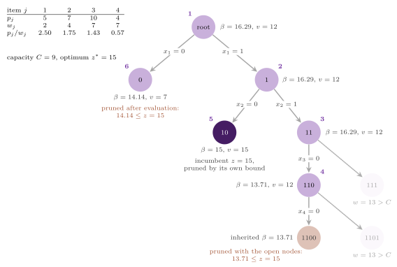
The example of the chapter has the four items of Figure 13.1 and the capacity \(C = 9\). Its optimum is 15 (the items 1 and 3, numbered from 1 in the figures), while the greedy completion of the root takes the items 1 and 2 and gives 12. The root bound is \(5 + 7 + 10 \cdot 3 / 7 = 16.29\) (to two decimals, as in all the figures). A node is named by the decisions it fixes, e.g., 10 for "item 1 taken, item 2 left out".
13.3 The sequential search¶
The sequential search BranchAndBoundSearch
(BranchAndBound.h:1206, or the function
branch_and_bound( p , options ), whose declarations, without their bodies,
are
[[nodiscard]] BBSolution< typename P::node_type , bb_value_t< P > >
branch_and_bound( const P & problem ,
                  const BasicBBOptions< bb_value_t< P > > & o = {} );
[[nodiscard]] BBSolution< typename P::node_type , bb_value_t< P > >
branch_and_bound( const P & problem ,
                  std::vector<
                    BBLeaf< typename P::node_type , bb_value_t< P > > > seeds ,
                  const BasicBBOptions< bb_value_t< P > > & o = {} );
for a model P of BranchAndBound) keeps the open nodes
in a queue Q, ordered by the key of the selection
(§13.5), and, with the plunging selection, a node \(d\) of
the dive, which is extracted next. Its pseudocode, which is that of the
Doxygen comment of BranchAndBound.h, is the following;
\(R\) is the set of the nodes it starts from (the root, unless the caller gives
others, §13.11).
Algorithm 13.3 (Sequential branch-and-bound).
 1  procedure B&B(R)          ▷ the nodes to start from, {root} by default
 2     z ← the given incumbent, or ∞;  Q ← R;  d ← nil  ▷ d: the dive
 3     while Q ≠ ∅ or d ≠ nil do
 4        βmin ← the least bound of Q and of d
 5        if a limit is reached and not PRUNABLE(βmin) then break
 6        if PRUNABLE(βmin) then the nodes of Q and d are leaves;  break
 7        n ← d if d ≠ nil, else the first node of Q, removed;  d ← nil
 8        K ← PROCESS(n)
 9        if the selection is plunging and K ≠ ∅ then
10           k ← the node of K of least bound
11           βmin ← min(the least bound of Q, β(k))
12           if z = ∞ or β(k) ≤ βmin + γ (z − βmin) then d ← k, from K
13        push the nodes of K in Q
14     the nodes left in Q and d are leaves             ▷ open by a limit
15     return z, its node, and the bound min(z, least bound of the leaves)
16  procedure PROCESS(n)
17     if PRUNABLE(β(n)) then n is a leaf (pruned);  return ∅
18     cutoff(z);  (β', infeasible, v) ← evaluate(n)
19     if infeasible then n is a leaf (infeasible);  return ∅
20     β(n) ← max(β(n), β')
21     if v is given and v < z then z ← v;  n is the node of z
22     if PRUNABLE(β(n)) then n is a leaf (pruned or feasible);  return ∅
23     K ← ∅;  cutoff(z)
24     for each child m of n, with its estimate e, given by branch(n) do
25        β(m) ← max(β(n), e)
26        if PRUNABLE(β(m)) then m is a leaf (pruned)
27        else K ← K ∪ {m}
28     if n has no child then n is a leaf
29     return K
30  procedure PRUNABLE(β)
31     if z = ∞ then return β = ∞
32     return β ≥ z − max(τ_a, τ_r |z|)
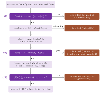
A node is thus tested three times (Figure 13.2): (i) when it is extracted (line 17), against an incumbent that may have improved since its generation, (ii) after its evaluation (line 22), against the bound it has just obtained, and (iii) when it is generated (line 26), against its inherited bound. A node that survives the second test is branched, also when it has a feasible value, since its subtree may hold better values than the one found. Line 6 is the termination test: as soon as the least bound of the open nodes cannot improve \(z\), neither can any of them, and all of them would be pruned at their extraction. All the searches of the library but the MultiQueue, which does not know the least bound of its queues (§13.8), use this test, and they also end when Q is empty or a limit is reached; as in the pseudocode, the emptiness of line 3 and the termination test come before the limits of line 5, so that a search whose last evaluation reaches the node limit with no open node left, or with none that can improve \(z\), ends as optimal. With best-first the test at line 6 often (but not always) ends the search while Q still holds many nodes, i.e., those generated before the incumbent was found and never extracted since.
The procedure PROCESS is detail::bb_process()
(BranchAndBound.h:1157). All the searches of the
library share it, each with the incumbent it sees (a function inc() that
returns \(z\) in the minimization) and with the function improve by which it
offers a feasible value; the children that survive line 26 go to a function
push of the caller, which puts them in its queue or in its messages.
The leaves go to a record of the worker, detail::BBFrontier
(BranchAndBound.h:884), which keeps the least bound
low of the leaves that lower the bound of the search and, only with
keep_frontier, the leaves themselves.
Algorithm 13.4 (The record of the leaves of a worker).
1  procedure LEAF(n, β, kind, lowers)          ▷ a leaf n of bound β
2     if lowers then low ← min(low, β)
3     if keep_frontier then append (n, β, depth(n), kind) to the leaves
4  procedure LEAVES(Q, kind)                   ▷ all the nodes of a queue
5     low ← min(low, the least bound of Q)
6     if keep_frontier then append each node of Q with its bound and depth
7     Q ← ∅
8  procedure MERGE(L')                         ▷ the record of another worker
9     low ← min(low, low of L');  append the leaves of L'
In PROCESS, an infeasible leaf (line 19) and a node with no children
(line 28) are recorded with lowers false: the former has no element,
and the latter is solved by Assumption (A3) of §13.4, its
value having been offered to \(z\) at line 21. The leaves of the three
tests are of the kind pruned, or feasible at line 22 when the node
gave a feasible value, and those left by a limit (line 14) of the kind
open. A child pruned at line 26 is copied into the record only with
keep_frontier; otherwise only its bound enters low.
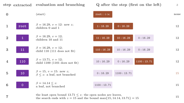
Figure 13.3 traces Algorithm 13.3 on the example. The greedy completion of the root gives \(z = 12\) at once. Then the search goes down the right branch, whose nodes inherit the bound \(16.29\) (the ties among equal keys are broken in favor of the last node pushed, cf. §13.5); the node 110 has the bound \(13.71\), which is still above \(z = 12\), and is branched. The node 10 gives the optimum 15 and is pruned by its bound, and the node 0 is pruned after its evaluation. Finally, the open node 1100, whose inherited bound is \(13.71 \le 15\), ends the search at line 6 without being evaluated; six nodes are evaluated in all.
13.4 Correctness and the reported bound¶
We now prove that Algorithm 13.3 returns a value within the tolerance of the optimum when no limit stops it, and that the bound it reports is a bound on the optimum whatever the status. We need four assumptions on the problem, which the concept cannot check:
- (A1) the children of a node cover its subset: \(X(n) \subseteq X(n_1) \cup \cdots \cup X(n_k)\);
- (A2) the bound of an evaluation, the estimate of a child and the bound given with each node of \(R\) are lower bounds: \(\beta'(n) \le v(x)\) for every \(x \in X(n)\), \(e(m) \le v(x)\) for every \(x \in X(m)\), and likewise for the nodes of \(R\) (the root starts with \(-\infty\));
- (A3) a node has no child only if it is solved, i.e., if its subset is empty or its evaluation gives a feasible value \(v\) with \(v \le v(x)\) for every \(x \in X(n)\);
- (A4) every chain of branchings is finite, e.g., because the subsets shrink strictly and \(X\) is finite.
The knapsack satisfies them, as we now show; in its case \(X(u)\) is the set of the \(x \in \{0, 1\}^n\) that agree with the node \(u\) on the items \(0, \ldots, k - 1\) and fit in the capacity.
Lemma 13.2 (The knapsack satisfies the
assumptions). With or without explicit_children, and with values of a
floating point or of an integer type, the knapsack of Algorithms 13.1
and 13.2 satisfies (A1) to (A4), the bounds being read in the
minimization of the negated profits.
Proof. (A1) Let \(x \in X(u)\) with \(k < n\). If \(x_k = 0\), then
\(x \in X(c)\). If \(x_k = 1\), then \(W(u) + w_k \le \sum_j w_j x_j \le C\),
so that the child \(t\) is generated at line 5 of Algorithm 13.2, and
\(x \in X(t)\). (A2) If \(W(u) > C\), then \(X(u) = \emptyset\) and the node
is reported infeasible; otherwise the bound of Algorithm 13.1 is at
least the profit of each \(x \in X(u)\) by Lemma 13.1, and
so is its floor for an integer type, since the profits are integer. The
estimate \(\infty\) of a child is a trivial bound, and with
explicit_children the estimate is the bound of the child, or \(\infty\)
if it does not fit. (A3) BRANCH gives no child only when \(k = n\); then
\(X(u)\) holds at most the vector of the node, and if it fits its profit
is \(P(u)\), the greedy value of line 7 of Algorithm 13.1, while if it
does not fit the node is infeasible. (A4) Each child fixes one item
more than its parent, and therefore every chain of branchings has at
most \(n\) steps. \(\square\)
We also need the threshold to behave well when \(z\) improves.
Lemma 13.3 (The threshold is monotone). If \(\tau_r \le 1\), the threshold \(\theta(z) = z - \max \{ \tau_a, \tau_r |z| \}\) is nondecreasing in \(z\), and so is its version for an integer type, \(z - \max \{ \tau_a, \lfloor \tau_r |z| \rfloor \}\).
Proof. One has \(\theta(z) = \min \{ z - \tau_a, \; z - \tau_r |z| \}\), the minimum of two functions of \(z\). The first is increasing, and the second has slope \(1 - \tau_r \ge 0\) for \(z > 0\) and \(1 + \tau_r\) for \(z < 0\); hence, both are nondecreasing, and so is their minimum. For the integer version, a unit increase of \(z\) changes \(\lfloor \tau_r |z| \rfloor\) by at most \(\lceil \tau_r \rceil \le 1\), so that \(z - \lfloor \tau_r |z| \rfloor\) does not decrease, and the same argument applies. \(\square\)
The condition \(\tau_r \le 1\) is not checked by the library. With a larger relative tolerance the threshold of a positive incumbent falls when the incumbent rises, which one hardly wants (a relative gap of more than 100% accepts any value of the same sign). We call open, at a given moment of Algorithm 13.3, the nodes of Q and the node \(d\) of the dive.
Lemma 13.4 (The invariant). Under (A1) to (A3) and with \(\tau_r \le 1\), at the start of each iteration of the loop at line 3 every \(x \in X(R)\) with \(v(x) < \theta(z)\) belongs to \(X(n)\) for some open node \(n\), where \(X(R)\) is the union of the subsets of the nodes of \(R\).
Proof. We proceed by induction on the iterations. At the start the open nodes are those of \(R\), and the claim holds. Assume it at the start of an iteration, which either breaks (and then there is no next iteration) or removes a node \(n\) from the open ones at line 7 and processes it. First, \(z\) can only decrease (line 21), and then so does \(\theta(z)\) by Lemma 13.3; hence, the set of the \(x\) to be covered can only shrink. Second, the elements of \(X(n)\) below the threshold are covered again after PROCESS, in each of its four outcomes. If \(n\) is pruned at line 17 or 22, then \(\beta(n) \ge \theta(z)\); since \(\beta(n)\) is the maximum of \(\beta'(n)\) and of bounds of supersets of \(X(n)\), it is a bound of \(X(n)\) by (A2), and no element of \(X(n)\) is below the threshold. If \(n\) is infeasible (line 19), \(X(n)\) is empty. If \(n\) has no child, each \(x \in X(n)\) has \(v(x) \ge v \ge z \ge \theta(z)\) by (A3), where \(v\) is its feasible value, offered at line 21. Otherwise, by (A1), each \(x \in X(n)\) is in the subset of a child \(m\), which is either pruned at line 26 (and then \(v(x) \ge \beta(m) \ge \theta(z)\) by (A2)) or put in Q or in \(d\) at lines 12 and 13. \(\square\)
Theorem 13.5 (Correctness and finiteness). Under (A1) to (A4) and with \(\tau_r \le 1\), Algorithm 13.3 performs a finite number of iterations. If no limit stops it, then either \(z < +\infty\) and
where \(z^*_R = \min \{ v(x) : x \in X(R) \}\), or \(z = +\infty\) and \(X(R)\) is empty (when no initial incumbent is given).
Proof. We note that each iteration that does not break removes one
node from the open ones and adds only children of it; hence, each node
of the trees below the nodes of \(R\) is processed at most once for each
node of \(R\) above it. The set \(R\) is finite, and by (A4) and by
König's lemma so are these trees, since each node has finitely many
children (branch() returns); hence, so is the number of iterations.
If no limit
stops the search, it ends at line 3 with no open node, or at line 6 with
each open node of bound at least \(\theta(z)\). In both cases Lemma
13.4 shows that no \(x \in X(R)\) has \(v(x) < \theta(z)\),
i.e., \(z^*_R \ge \theta(z)\), which is the claim. If \(z = +\infty\), then
\(\theta(z) = +\infty\) in the sense of the test at line 31, and no \(x\)
exists. \(\square\)
Note that with an initial incumbent value below the optimum, the search
ends with that value and no node (the test bb checks this case). The
value \(z\) of Theorem 13.5 is in any case a value found or
given, and the inequality bounds it from above. When a limit stops the
search, or when the tolerances are positive, the leaves give a bound on
the optimum, which is the bound of BBSolution. The leaves of a
search are the nodes it does not branch: those pruned at the three
tests, the infeasible ones, those with no child, and those left open by
a limit (lines 6 and 14). Algorithm 13.4 records the least bound low
of those that lower the bound, i.e., all but the infeasible ones and
those with no child, and it keeps the leaves themselves only with
keep_frontier.
Theorem 13.6 (The reported bound). Under (A1) to (A3), whatever the status of the search,
and therefore the gap \(z - L\) reported by BBSolution bounds
\(z - z^*_R\).
Proof. If \(X(R)\) is empty there is nothing to prove. Otherwise we let
\(x^*\) be optimal over \(X(R)\). By (A1), the subsets of the leaves cover
\(X(R)\); the argument is that of Lemma 13.4 with no
threshold, since each node of the tree is either branched (and then
covered by its children) or a leaf, the nodes still open when the search
ends being leaves of kind open. Let \(l\) be a leaf with \(x^* \in X(l)\).
It is not infeasible, since \(X(l) \ne \emptyset\). If it has no child,
then \(z^*_R = v(x^*) \ge v \ge z \ge L\) by (A3), where \(v\) is its
feasible value, offered to the incumbent. Otherwise it lowers the bound,
and \(\beta(l) \le v(x^*)\) by (A2), so that again \(z^*_R \ge L\).
\(\square\)
The leaf that has no child is excluded from \(L\) because its subtree is
the node, whose value is offered to \(z\); the infeasible leaf is excluded
because its bound is \(+\infty\). Note that the bound \(\beta(l)\) of a leaf
pruned at its generation or at its extraction is an inherited one, which
is usually weaker than the bound its evaluation would give. The reported
bound is therefore valid but not necessarily the best one available; it
is exact (equal to \(z\)) when the search ends with zero tolerances and no
limit, since then each leaf has \(\beta(l) \ge z\). We remark that the
theorem is stated for Algorithm 13.3, which prunes by its own \(z\). With
shared_incumbent the search prunes by the least \(c\) of \(z\) and of the
values read, which are not offered to \(z\), and the same proof gives
only \(z^*_R \ge \min \{ L, c \}\): a leaf with no child whose value is
not better than \(c\) is in neither \(z\) nor \(L\) (this is why the bound of
Exercise 13.2 is at most the optimum). On the example the
bound is \(\max \{ 15, 14.14, 13.71, 15 \} = 15\) in the maximization, and
the gap is 0.
13.5 The selection rules¶
Lemma 13.4 holds whatever the order in which the open nodes
are extracted. Therefore the order is a policy, the Selection of the
options (BranchAndBound.h:137), which decides how
many nodes are evaluated and how much memory the queue takes, while the value
returned is within the tolerance anyway. In the queue we order the nodes by a
key: the bound with best-first and plunging, minus the depth with
depth-first, the depth with breadth-first, and the estimate of the
problem with best-estimate (the bound, if the problem gives no
estimate). Among equal keys the last node pushed comes first, but with
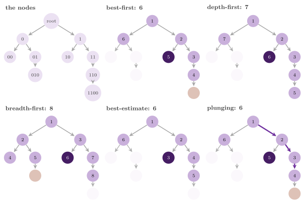
breadth-first, where the first comes first. Figure 13.4
shows the five rules on the example.
Best-first¶
With best-first the node of least bound is extracted first. When the bound of a node does not depend on the order of the search, best-first evaluates the fewest nodes, in the following sense.
Proposition 13.7 (Best-first evaluates the
necessary nodes, and "few" others). Assume (A1) to (A4), zero tolerances,
no limit, no initial incumbent below \(z^*\), and that the evaluation of
a node depends only on the node (no cutoff). Call a node critical
if its inherited bound and the evaluated bounds of all its ancestors
(taken as \(+\infty\) for an infeasible one) are less than \(z^*\). Then (i)
each selection evaluates each critical node, and (ii) best-first
evaluates only nodes whose inherited bound is at most \(z^*\).
Proof. (i) We argue by induction along the path from the root. At the start the root is open. A critical node \(m\) that is open is never pruned at line 6, 17 or 26, since its bound is less than \(z^* \le z\); since the search ends with no open node of bound below \(z\) (Theorem 13.5), \(m\) is extracted and evaluated. If \(m\) has a critical child, its evaluated bound is less than \(z^*\) by the definition, and it is not pruned at line 22; it is therefore branched, and its critical children, whose inherited bounds are less than \(z^* \le z\), survive line 26 and are open. (ii) While \(z > z^*\), some open node \(m\) holds an optimal \(x^*\) (Lemma 13.4, since \(v(x^*) = z^* < z\) and the tolerance is 0), and \(\beta(m) \le z^*\) by (A2); best-first extracts a node of least bound, which is therefore at most \(z^*\). Once \(z = z^*\), a node extracted with \(\beta \ge z^*\) is pruned at line 17 before its evaluation. \(\square\)
Hence, the nodes evaluated by best-first are the critical ones plus some
of those whose bound equals \(z^*\), and how many of the latter depends on
the ties (the test bb checks the optimum of every selection, not the
number of the evaluations). This result is the counterpart of the
optimality of A\(^*\) among the algorithms that use the same heuristic
(Chapter 2), and it fails in two ways that are
common in practice: with cutoff, the evaluation of a node depends on
the incumbent, and with a relaxation solved by a warm start from the
previous node it depends on the order. Its price is the memory: the
queue may grow to a "large" part of the tree before an incumbent is found,
since each open node whose bound is below the incumbent of the moment
stays in it until it is extracted.
Depth-first branch-and-bound¶
With depth-first the deepest node is extracted first, which typically
finds feasible values early and keeps the queue "small". This is the
depth-first B&B (DFBnB) of the literature of heuristic search, i.e., a
depth-first search that prunes each node whose bound is not less than
the best value found so far. It is an anytime algorithm, since an
incumbent is available (through on_incumbent) long before the search
ends. Since the children of a node have the same depth and the ties are
broken in favor of the last pushed, the child that a problem gives last
to the sink is the first one extracted. A problem that wants its
children tried by increasing bound, as DFBnB with sorted successors
does, gives them by decreasing bound (the knapsack gives the child that
takes the item last, which is the child of the greedy order). The
version of DFBnB on the graph of a Domain, without a queue, is in
Chapter 4. Here, instead, the search works
on any BranchAndBound problem, e.g., on the tree of the partial tours
of the traveling salesperson problem that the benchmark uses
(§13.20); there the first complete tour is reached after
one evaluation per level of the tree, and from then on it prunes the
partial tours whose bound is not less than its cost.
Proposition 13.8 (The memory of depth-first). With the depth-first selection, started from the root only, Q never holds more than \((b - 1) D + 1\) nodes, where \(b\) is the largest number of children of a node and \(D\) the depth of the tree.
Proof. We show that, at the start of each iteration, the nodes of Q at each depth \(\delta \ge 1\) are children of one node, and that Q holds at most \(b - 1\) of them at each depth but its deepest one, where it holds at most \(b\). This holds at the start, when only the root is in Q. An iteration extracts a node \(n\) of the deepest level \(\delta\) of Q, which leaves at most \(b - 1\) nodes at depth \(\delta\), all siblings of \(n\). It pushes at most \(b\) children of \(n\) at depth \(\delta + 1\), where Q had no node. The levels above \(\delta\) are unchanged, and each of them lost one node (the ancestor of \(n\) at that depth) when it was the deepest; hence, each holds at most \(b - 1\) nodes. Summing over the depths \(1, \ldots, D\) gives \((b - 1)(D - 1) + b = (b - 1) D + 1\). \(\square\)
Depth-first pays in the evaluations: it may evaluate "many" nodes that best-first would prune, i.e., those whose bound lies between \(z^*\) and the incumbent of the moment (the depth-first tree of Figure 13.4 evaluates 1100, which best-first prunes unevaluated).
Breadth-first, best-estimate and plunging¶
Breadth-first extracts the shallowest node, the oldest among those
of the same depth. It is rarely the right choice for a B&B whose
feasible values come only from the leaves (on the example it is the
worst of the five, with eight evaluations), but it gives the nodes of a
level together, which some uses may want. Best-estimate extracts the
node of least estimate of the best feasible value in its subtree, which
the problem gives by estimate( n ) (for the knapsack, its greedy
value). It aims at finding a "good" incumbent early, while the bound
still drives the pruning and the termination test.
Plunging is the usual compromise: the best child of the node just
branched is extracted next (a dive) as long as its bound is within
the fraction \(\gamma\) (plunge_gap) of the gap from the least open
bound \(\underline{\beta}\), i.e., while
and always while there is no incumbent; when the dive stops, the search
goes back to best-first (lines 9 to 12 of Algorithm 13.3). With \(\gamma
= 0\) a dive continues only into a child whose bound equals the least
open bound. With \(\gamma = 1\) it continues into each child that is not
pruned, which makes the search depth-first in the order of the bound of
the children and best-first among the nodes left behind (the test bb
runs both extremes). One can expect a dive to be "cheap" when the
evaluator keeps the state of the last node, e.g., a relaxation solved
again from the basis of its parent. In the code
(BranchAndBound.h:1336) the child \(k\) of line 10 is
the last of the children of least bound, and the test of line 12 is
BBValueTraits::within(), which computes the right-hand side in the type of
the values for a floating point type and in long double for an integer one,
which cannot overflow. The test is false when \(\underline{\beta}\) is not finite
(e.g., \(-\infty\) for a node given back with an unknown bound,
§13.11), and then no dive is taken while an incumbent exists.
The queue¶
The open nodes are kept in a BBQueue
(BranchAndBound.h:617). Its nodes are in an array of
slots, each holding a node with its bound and its depth, with a free list,
since a node is destroyed when it is branched (in A\(^*\) a node stays in CLOSED,
while here no structure refers to a node after its processing). Its order is a
pair of indexed 4-ary heaps on the indices of the slots, taken from the default
data structures of the library (Chapter 3): one
by the key of the selection, with the number of the push to break the
ties, and one by the bound. With the second heap one has the least open
bound in \(O(1)\), which the termination test at line 6 and the reported
bound need when the key is not the bound. Each change, the pop
included, is made on both heaps at the places of the index, and the
heaps grow by doubling with the slots. Figure 13.5 shows a
pop with the depth-first selection.
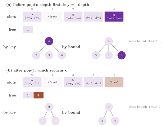
A push takes a free slot (or a new one), stores the node and pushes its index in both heaps, the key paired with the number of the push, complemented unless the order is first in, first out, and a pop takes the index of least key out of both heaps and frees its slot. In pseudocode, with \(H_K\) the heap of the keys and \(H_B\) that of the bounds, both on the indices of the slots, and \(s\) the number of the pushes so far:
Algorithm 13.5 (The queue of the open nodes).
 1  procedure PUSH(n, β, δ, key)          ▷ a node, its bound, depth, key
 2     i ← a slot of the free list, removed, or a new slot
 3     if i is beyond the capacity c of the heaps then
 4        rebuild both heaps with capacity 2i + 16, inserting their indices
 5     s ← s + 1;  slot[i] ← (n, β, δ)
 6     insert i in H_K with the key (key, s) if breadth-first, else (key, −s)
 7     insert i in H_B with the key β
 8  function POP()
 9     i ← the top of H_K;  remove i from H_K and from H_B
10     put i on the free list;  return the content of slot[i], emptied
11  function BESTBOUND()
12     return the key of the top of H_B, or ∞ if the queue is empty
Here \(-s\) stands for the complement of \(s\) in 64 bits, which orders the pushes in the opposite way. The costs are the following.
Proposition 13.9 (The queue). Let \(N\) be the number of the open nodes and \(M\) the largest number of open nodes at any time. Then (i) the pairs (key, \(\pm s\)) are distinct, so that POP returns a well-defined node, the least key first and, among equal keys, the last pushed (the first pushed with breadth-first); (ii) BESTBOUND and the first node take \(O(1)\) time, POP takes \(O(\log N)\) time, and PUSH takes \(O(\log N)\) time but for the rebuilding of line 4, whose total cost over a sequence of pushes is \(O(M \log M)\), i.e., \(O(\log M)\) amortized per push when at least \(M\) pushes are made; (iii) the queue uses \(O(M)\) memory, besides the nodes themselves.
Proof. (i) Each push takes a new value of \(s\), and the order on the pairs is lexicographic. (ii) In a 4-ary heap of \(N\) elements, an insertion moves an element up at most \(\lceil \log_4 N \rceil\) levels with one comparison per level, and the removal of an element whose position is known (the heaps are indexed by the slots) moves the last element up or down along one path of at most \(\lceil \log_4 N \rceil\) levels with at most 4 comparisons per level; a push makes one insertion in each heap and a pop one removal in each, and the free list is a stack. The top of a heap is its first element. The rebuilding of line 4 happens when the index \(i\) reaches the capacity \(c\), and sets it to \(2i + 16 > 2c\); the capacities are therefore at least doubled, and since \(i < M + 1\) (a slot is new only when all the slots hold nodes), the rebuildings insert at most \(M\) indices each, with capacities \(c_1 < c_2 < \cdots\) at least doubling up to \(O(M)\), i.e., \(O(\sum_t c_t \log M) = O(M \log M)\) in all. (iii) The slots are at most \(M + 1\), and the heaps have capacity \(O(M)\). \(\square\)
The move of one node per push and per pop is apart, and so is the destruction of the node of a slot. These costs are usually negligible when the evaluation solves a relaxation, which is the case the layer is meant for. They matter only for problems whose bound costs about as much as a "few" comparisons; the knapsack of the tests is one, and it is therefore a test of the overheads of the schemes rather than of their intended use. One could also keep the bounds in a heap with lazy deletion, in which the indices popped by key stay until they reach its top: this saves the second walk of a pop, but the least bound must then skip the stale entries, while the indexed pair keeps the bound of each index exact.
We can now bound the cost of a whole sequential search in terms of the
work of the problem. In the following, an evaluation costs at most
\(T_e\) time and a branching, i.e., a call of branch(), at most \(T_b\)
time besides the calls of sink.
Proposition 13.10 (The cost of the sequential
search). Let Algorithm 13.3 process \(E\) nodes (line 8), generate \(G\)
children, and let \(M\) be the largest number of its open nodes. Then it
makes at most \(E\) evaluations and \(E\) branchings, and takes
\(O(E (T_e + T_b + \log M) + G \log M)\) time besides the leaves
recorded at its end (lines 6 and 14, \(O(M)\) time) and the calls of
shared_incumbent and of the clock (one per iteration). It uses \(O(M)\)
memory for the open nodes, plus the leaves kept with keep_frontier.
Proof. We note that each iteration of the loop at line 3 that does not break extracts one node (line 7), by POP in \(O(\log M)\) time (Proposition 13.9) or from the dive, and processes it. PROCESS makes at most one evaluation (line 18) and one branching (line 24), and for each child it makes \(O(1)\) work and either a record in \(O(1)\) (Algorithm 13.4, amortized for the append) or a push, in \(O(\log M)\) amortized time; with plunging, lines 9 to 12 scan the children once. The least bound of line 5 is BESTBOUND, in \(O(1)\). The memory holds the queue (Proposition 13.9), the node of the dive, the children of one node and the record of the leaves. \(\square\)
Note that \(E \le |R| + G\), since each node processed was pushed once, and that \(G \le b E\) when no node has more than \(b\) children; hence the overhead of the search is \(O(b \log M)\) per evaluation, which is negligible when \(T_e\) is the time of a relaxation.
13.6 A\(^*\) as a special case¶
Nau, Kumar and Kanal [17] formulated a
general B&B of which A\(^*\) (and AO\(^*\)) are special cases. In our terms,
A\(^*\) on a tree is the B&B in which a node is a path from \(s_0\) to a
state \(u\), and its subset is the set of the paths to a goal that extend
it. Its bound is \(f(u) = g(u) + h(u)\), which is a lower bound on the
cost of these paths when \(h\) is admissible, and a goal gives the
feasible value \(g(u)\). In the benchmark of the chapter we use this
construction (TourTree in
tools/BranchAndBoundBench.cpp) on the traveling
salesperson problem of Chapter 14, whose search space is
a tree: evaluate() returns \(g + h\) as the bound and \(g\) as the feasible value
of a goal, and branch() gives each successor with its \(g + h\) as estimate.
Proposition 13.11 (A\(^*\) as best-first B&B). On the tree of the paths from \(s_0\), with an admissible heuristic, \(h = 0\) on the goals, nonnegative edge costs, zero tolerances and the best-first selection, the first goal that Algorithm 13.3 evaluates has the optimal cost \(C^*\), and the search ends at the next test of line 6 with no further evaluation.
Proof. We first observe that, while no goal of cost \(C^*\) has been evaluated, \(z > C^*\) and some open node \(m\) lies on an optimal path (Lemma 13.4); its bound is the largest \(f\) along that path up to \(m\) (by the pathmax of §13.2), which is at most \(C^*\) by admissibility. Let \(u\) be the first goal evaluated; when it was extracted it had the least bound among the open nodes, so that \(\beta(u) \le \beta(m) \le C^*\), while \(\beta(u) \ge f(u) = g(u) \ge C^*\) since \(h(u) = 0\). Hence \(g(u) = C^*\), the evaluation sets \(z = C^*\), and the least bound of the open nodes is at least \(\beta(u) = C^*\) (best-first extracted \(u\) as a node of least bound, and the children pushed since then have bounds of at least that of their parent). The test at line 6 then prunes all of them. \(\square\)
We remark that the proof shows the role of pathmax. With an inconsistent heuristic \(f\) may decrease along a path, but the inherited bound does not, and best-first on the inherited bound extracts the nodes in nondecreasing order of their key. Still, the two searches differ in two respects. First, a graph has duplicates, i.e., several paths to the same state, of which only the cheapest matters. A\(^*\) detects them with CLOSED and keeps one node per state, while a B&B tree has none and needs no closed list; on a graph with many duplicates the B&B view enumerates the paths, and A\(^*\) is the right tool. Second, A\(^*\) stops at the first goal extracted, while a B&B goes on until no open node can improve the incumbent. In a general B&B the first feasible value is often not optimal, and a node with a feasible value may hold better values below, as the root and the node 1 of Figure 13.1 do (value 12, and the optimum 15 below). This is why the two layers of the library share the parallel schemes and the executors, but not the node table and the OPEN lists of A\(^*\). For the same reason SafePBNF and PA\(^*\)SE (Chapter 11 and Chapter 8) have no counterpart here: they exist to handle the duplicates and the re-expansions, which a tree does not have.
13.7 What a parallel search has to guarantee¶
We now turn to the parallel B&B searches of the library, all of which build one tree with \(p\) workers and differ in how they share the open nodes and the incumbent. In the classification of Gendron and Crainic [16] they are of the second type, i.e., the parallelism is in the exploration of the tree. Any parallelism inside the evaluation of a node (their first type) is left to the problem, and the search of several trees at once (their third type) is provided only at the start, by the racing ramp-up of §13.15. Within the second type the searches are asynchronous, but for the deterministic rounds. They keep either one pool of open nodes (the shared queue, the MultiQueue, the farm and the rounds, §13.8) or one pool per worker (the distributed queues, the processes of MPI, the work stealing and the SelfSplit, §13.9, and the skeletons, the hubs and the intervals of leaves of §13.14, §13.17 and §13.18).
Note that the invariant of the sequential search holds for a parallel
one if the open nodes are taken in a wider sense: the nodes in any
queue, those held by a worker (being processed, or the next node of a
dive), and those traveling in a message, a task, an offer of a steal or
a slot of a round. Since the incumbent is shared, each worker prunes by
the value it sees, which may be older than the current one; the
following lemma shows that this is safe. The incumbent is an object of
the class BBIncumbent
(ParallelBranchAndBound.h:227), whose two
operations are lines 1 to 8 of the following algorithm; lines 9 to 17 give the
dive and the test of the limits, which all the parallel searches share and
which are described at the end of this section.
Algorithm 13.6 (The shared incumbent, the dive and the limits of the parallel searches).
 1  function VALUE()                       ▷ read by the workers to prune
 2     return z, an atomic read with relaxed order if the values have a
          lock-free atomic type, else a read under the lock M
 3  function IMPROVE(v, n)                 ▷ the feasible value v of n
 4     if the values are atomic and v ≥ VALUE() then return false
 5     lock M
 6     if v ≥ z then unlock M;  return false
 7     z ← v;  the node of z ← n;  call on_incumbent(v);  unlock M
 8     return true
 9  function DIVE(K, bl, z)                ▷ bl: the least open bound known
10     if K = ∅ then return nil
11     if depth-first then return the last node of K
12     if not plunging then return nil
13     k ← the last node of K of least bound;  bl ← min(bl, β(k))
14     if z = ∞ or (bl is finite and β(k) ≤ bl + γ (z − bl)) then return k
15     return nil
16  function LIMIT(c)                      ▷ c: the nodes counted so far
17     return (node_limit > 0 and c ≥ node_limit) or the time limit has
          passed, setting the flags of the limit (and of the time) if so
Lemma 13.12 (The shared incumbent). In
BBIncumbent (ParallelBranchAndBound.h:227),
(i) the value never increases, (ii) each value it takes is the initial one or a
feasible value offered by a worker, and (iii) the stored node is a node of the
stored value whenever the lock is free, and the callback on_incumbent
is called with strictly decreasing values. Hence, a worker that prunes
by a value it read earlier prunes a subset of what it would prune by
the current one.
Proof. We note that the value changes only at line 7 of Algorithm 13.6, under the lock \(M\), after the test of line 6, which reads the value under the same lock. That value is the last one stored, since all the stores are made under \(M\), which orders them; the store of the node and the call of the callback follow under \(M\). The test of line 4 only returns early, when \(v\) is not below a value that \(z\) had at some moment, which is not below the current one, since each store of line 7 lowers \(z\) (line 6). This gives (i), (ii) and (iii). A worker that read the value \(z' \ge z\) earlier (the read without the lock may return an older value) prunes \(\beta \ge \theta(z')\), which implies \(\beta \ge \theta(z)\) by Lemma 13.3. \(\square\)
In the library, when the type of the values has a lock-free
std::atomic, the value is an atomic variable on a line of cache of its
own, which the workers read without a lock and with relaxed order when
they prune. The first test of improve() discards without the lock the
values that are not better than the one seen, and only an improvement,
which is usually "rare", takes the lock. For another type (e.g., the
rationals of an exact arithmetic) the value is read under the lock too.
Theorem 13.13 (Correctness of a parallel
search). Under (A1) to (A4) and with \(\tau_r \le 1\), let a parallel
search process each node by PROCESS with an incumbent value read from
BBIncumbent (or, over MPI, received from it,
§13.9), and let it move nodes only between the places of
the wider open set. Then at any moment every \(x \in X(R)\) with
\(v(x) < \theta(z)\), \(z\) the current incumbent, belongs to \(X(n)\) for a
node \(n\) of the wider open set. Hence, if the search ends only when the
wider open set is empty, or when each node in it has a bound of at
least \(\theta(z)\), its value satisfies
Theorem 13.5, and the bound computed from the leaves of
all the workers satisfies Theorem 13.6.
Proof. We note that the proof of Lemma 13.4 applies to each step of each worker, the steps of different workers being interleaved. A step that moves a node keeps it in the wider open set. A step of PROCESS replaces the node by its children or makes it a leaf, and a leaf pruned by a value \(z'\) read earlier has no element below \(\theta(z') \ge \theta(z)\) (Lemma 13.12). An improvement of \(z\) shrinks the set to be covered. Finally, the leaves collected by the workers cover \(X(R)\) together with the wider open set, which gives the bound as in Theorem 13.6 once the nodes left open are added as leaves (each search does so at its end). \(\square\)
All the schemes below satisfy the hypotheses, but for the SelfSplit,
whose workers prune by incumbents of their own and which
Theorem 13.23 treats apart. What remains to prove for
each is that it ends only in one of the two situations of Theorem
13.13, and that it does end. Of the two, the end is the
delicate part: a worker that finds no node cannot conclude that none
exists, since another worker may be about to generate some (cf. the
general discussion of the termination of parallel searches in Chapter
8 and Chapter
9). Also, one can stop each scheme at a
node or time limit (LIMIT, lines 16 and 17 of Algorithm 13.6,
detail::bb_limit(),
ParallelBranchAndBound.h:360), and the node
that a worker holds when it sees the limit becomes an open leaf. In every
search the count \(c\) is that of the evaluations, i.e., of the calls of PROCESS
that reach line 18 (a node pruned at line 17 is not counted); in the shared
queue, the MultiQueue, the farm, the distributed queues and the work stealing
it is a counter shared by the workers, raised after each such call. The limit
is then exceeded by a bounded amount.
Proposition 13.14 (The node limit of the asynchronous schemes). Let a node limit \(L > 0\) be given, and no time limit. In the shared queue, the MultiQueue, the distributed queues and the work stealing, the evaluations are at most \(L + p - 1\); in the farm, with batches of \(k\) nodes, at most \(L + p k\).
Proof. In the first four schemes a worker calls LIMIT on the counter \(c\) before it processes each node, the node of a dive included, and raises \(c\) after an evaluation. Consider the last evaluation that starts: at its test \(c \le L - 1\), i.e., at most \(L - 1\) evaluations had ended, and at most \(p - 1\) others were under way, one per other worker; hence the evaluations are at most \((L - 1) + (p - 1) + 1\). In the farm the master tests the limit when a task comes back and dispatches no task after the test has succeeded, while a worker tests it only after each evaluation, to stop the dive of the node, and completes the at most \(k\) nodes of its task. The evaluations that end after \(c\) has reached \(L\) belong to the tasks out at that moment or sent by the dispatch under way, which are at most \(p\) together, since the master never has more than \(p\) tasks out; each of them evaluates at most its \(k\) nodes, since no dive goes on once \(c \ge L\). \(\square\)
The bound counts the evaluations; the nodes pruned when extracted, which cost no evaluation, are not counted. The rounds, instead, never exceed the limit (Theorem 13.18), and over MPI each process stops at its share (§13.9).
Anomalies¶
Of course, the evaluations of a parallel search are not those of the sequential one, and they may be more or fewer (often, but not always, more). On the one hand, a worker may evaluate a node that the sequential search prunes by an incumbent which, in the parallel search, another worker finds only later (a detrimental anomaly, which is the search overhead of a B&B). On the other hand, a worker may find an incumbent earlier than the sequential search does and prune nodes that the latter evaluates (an acceleration anomaly, which gives a speedup larger than \(p\)). Lai and Sahni [149] showed that both occur in parallel best-first B&B, and that adding workers may even "slow" a search down; Gendron and Crainic [16] discuss them with the literature that followed. With the best-first selection the detrimental part is somewhat limited, since the nodes extracted by the workers are among the best open ones. It grows with the distance between the order of extraction and the sequential one, and this distance distinguishes the schemes below.
The dive in a parallel search¶
With depth-first and plunging, a worker of a parallel search goes on
with one child of the node it processed without putting it in a queue
(DIVE, lines 9 to 15 of Algorithm 13.6, detail::bb_dive(),
ParallelBranchAndBound.h:335). With
depth-first it is the last child, which the queue would extract next anyway.
With plunging it is the last child of least bound, if that bound is "close
enough" to the least open bound bl that the worker knows: the least bound of
the shared queue (read under its lock), that of the queue of the worker in the
distributed queues, over MPI and in the work stealing, the least open
bound of the moment at which the task was dispatched in the farm, and
the bound of the node processed in the MultiQueue. We write DIVE(\(K\))
for that child, nil if there is none; it stays in the wider open set as
a node held by the worker.
13.8 One pool of open nodes¶
The shared queue¶
In the shared queue (SharedBranchAndBound,
ParallelBranchAndBound.h:389) the workers
extract the nodes from one queue under a lock \(L\), evaluate and branch them
outside of it, and push the children back under it, as the workers of SPA\(^*\)
do with the states of A\(^*\) (Chapter 8); the child
of a dive stays with the worker. Its order of extraction is close to the
sequential one, from which it departs by the \(p\) nodes processed at
once and by the times at which the incumbents are found. Also, the lock
is rather "cheap" when the evaluation dominates, which is the usual case
of a B&B. The pseudocode, with a counter busy of the workers that hold
a node, is the following.
Algorithm 13.7 (The shared queue).
 1  procedure SHARED(R)       ▷ one queue Q, under the lock L, for all
 2     Q ← R;  busy ← 0;  done ← false
 3     in parallel, on each worker i = 0, ..., p − 1 do
 4        d ← nil
 5        loop
 6           if d ≠ nil then n ← d;  d ← nil
 7           else n ← NEXT();  if n = nil then return
 8           if a limit is reached then
 9              n is a leaf (open);  busy ← busy − 1;  done ← true;  return
10           K ← PROCESS(n)
11           lock L;  d ← DIVE(K);  push the nodes of K but d in Q
12           if d = nil then busy ← busy − 1
13           unlock L
14  procedure NEXT()
15     loop
16        if done then return nil
17        if Q = ∅ then                             ▷ read without the lock
18           if busy = 0 then
19              lock L;  if Q = ∅ and busy = 0 then done ← true;  unlock L
20           else wait a little
21           continue
22        lock L
23        if PRUNABLE(the least bound of Q) then
24           the nodes of Q are leaves (pruned);  Q ← ∅;  unlock L
25           continue
26        busy ← busy + 1;  n ← the first node of Q, removed;  unlock L
27        return n
Figure 13.6 shows two steps: a worker extracts a node,
raising busy, while another pushes the children of the node it
processed, lowering it.
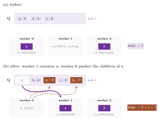
Proposition 13.15 (The end of the shared
queue). In Algorithm 13.7, (i) whenever \(L\) is free, busy is the
number of the workers that hold a node (extracted and not yet pushed
back, or kept for a dive); (ii) if a worker finds \(Q = \emptyset\) and
busy \(= 0\) under \(L\) (line 19), no node is open in the wider sense;
(iii) if the evaluations terminate, each worker returns.
Proof. (i) We observe that a worker raises busy under \(L\) in the
same critical section in which it takes a node from Q (line 26). It
keeps it raised while it processes the node and the nodes of its dive
(lines 6 and 10), and lowers it under \(L\) only in the critical section
in which it has pushed the children and kept no dive (lines 11 to 13),
or when it stops at a limit (line 9). (ii) The wider open set of this
scheme is Q and the nodes held by the workers (no node travels), and
both are empty. (iii) A worker loops in NEXT only while Q is empty and
busy \(> 0\), or while Q is not empty. In the first case some worker
holds a node, which it processes in finite time, and whose dive ends at
a leaf of the finite tree; that worker then pushes the children or
lowers busy. In the second case the worker takes a node or empties Q
at line 24. Since each node is processed once and the tree is finite
(A4), the loop ends by line 16 or 19. \(\square\)
The test of line 17 reads without the lock an atomic copy of the size
of Q. Hence, a worker that finds no node waits without taking
the lock, and with a growing pause, while the decision to stop is taken
under the lock, which makes the stale reads harmless. The counters
busy, the size of Q, the evaluations and the flag done sit on
separate lines of cache. Also, when the least bound of Q cannot improve
the incumbent, the whole queue becomes a set of leaves at once
(line 24). The push of the children (lines 11 to 13) holds the lock for
the time of the pushes of one node, i.e., \(O(|K| \log N)\) by
Proposition 13.9, and the extraction (lines 22 to 27) for one POP; each
node processed thus costs two critical sections, besides those of
line 19, and the lock of the incumbent only when it improves it.
The MultiQueue¶
The MultiQueue B&B (MultiQueueBranchAndBound,
MultiQueueBranchAndBound.h:129) is the
shared queue with the relaxed queue of MQA\(^*\) (Chapter
8). The open nodes are in a MultiQueue of Rihani,
Sanders and Dementiev [37], i.e., \(2p\) sequential
queues, each under a separate lock. A pop reads the least keys of two queues
drawn at random, without locks, and takes the least node of the better one; no
lock is common to all the workers. The price is a relaxed order of
extraction: indeed, a pop may return a node that is not the least of
all. In the sequential model of the MultiQueue (the nodes spread at
random, then removed by the better of two queues drawn at random) the
expected number of open nodes with a smaller key, the rank error,
converges, as the pops go on, to a value below
\(\frac{5}{6} \cdot 2p\), i.e., it is \(O(p)\)
(cf. [37] and
[38]). This is a result of the sequential
model with two new queues at each pop (the library draws two new queues
at each pop, i.e., with a stickiness of 1), which we do not prove here;
it does not cover the buffers of the queues nor the push of all the
children of a node into one queue, and we claim no bound on the rank
error of the library. Its termination test cannot use a
counter of busy workers, since there is no lock under which Q and the
counter are read together. It uses instead a counter \(m\) of the nodes
that are in the queue or held by a worker.
Algorithm 13.8 (The MultiQueue).
 1  procedure MULTIQUEUE(R)
 2     Q ← R;  m ← |R|;  done ← false
 3     in parallel, on each worker i = 0, ..., p − 1 do
 4        d ← nil
 5        while not done do
 6           if d ≠ nil then n ← d;  d ← nil
 7           else
 8              n ← a pop of Q, possibly nothing
 9              if no node was popped then
10                 if m = 0 then done ← true else wait a little
11                 continue
12              if PRUNABLE(the bound of n) then
13                 n is a leaf (pruned);  m ← m − 1;  continue
14           if a limit is reached then n is a leaf (open); done ← true; return
15           K ← PROCESS(n);  d ← DIVE(K)
16           m ← m + |K| − 1;  push the nodes of K but d in one queue of Q
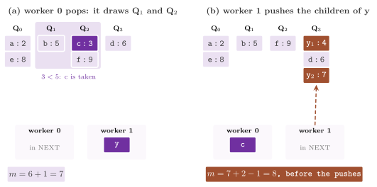
Proposition 13.16 (The end of the MultiQueue). In Algorithm 13.8, \(m\) is at any moment at least the number of the nodes in Q plus those held by the workers; hence, \(m = 0\) at line 10 means that no node is open, and the search then ends. If the evaluations terminate, each worker returns.
Proof. We first note that at the start \(m = |R|\), and the claim holds
with equality. A pop moves a node from Q to a worker and leaves \(m\)
unchanged, and a node pruned at line 13 leaves both and is subtracted.
At line 16 the node processed leaves and \(|K|\) children appear, of which
DIVE(\(K\)) is held by the worker and the others enter Q. Since \(m\) is
changed by \(|K| - 1\) in one atomic step before the pushes, between
this step and the end of the pushes \(m\) counts children not yet in Q,
which is an overcount and never an undercount. A worker that stops at a
limit sets done for all. For the second claim, note that a pop finds
no node only after a scan of all the queues found them empty. Hence, a
worker waits at line 10 only while \(m > 0\) and each counted node is held
by a worker or being pushed; those nodes are processed in finite time,
and the tree is finite. \(\square\)
The least bound of Q is not known, since each queue knows only its least
key. Hence, a node is pruned when popped (line 12) rather than with all
the others, and DIVE compares the children with the bound of the node
processed. The children of a node go into one queue under one lock (the
operation pushAll of the MultiQueue), which relaxes the rank somewhat,
as a stickiness of their number would, and saves a lock per child.
Furthermore, the values must be atomic with no lock (the concept
MultiQueueValue,
MultiQueueBranchAndBound.h:105), since the
MultiQueue keeps the least key of each queue in an atomic word that the pops
read without the lock. Similarly, the counter of the evaluations, which each
worker would update, is touched only when a node limit is set. In the code \(m\)
is the counter held, and line 16 is one atomic addition of \(|K| - 1\) (a
subtraction of 1 when \(K = \emptyset\), in the modular arithmetic of the
unsigned counter), made before the operation pushAll that moves the nodes of
\(K\) but \(d\) into one queue under its lock; the case of one child, which
replaces the node processed, needs no atomic operation. We expect the
MultiQueue to pay off only when an evaluation is so "fast" that the lock of the
shared queue is the bottleneck; when the evaluation dominates, its relaxed
order perhaps costs more evaluations than the lock costs time.
The master-worker farm¶
The farm (FarmBranchAndBound,
FarmBranchAndBound.h:104) is the master-worker
form of the shared queue, written as a farm with feedback, the pattern of
FastFlow [12], on the executor of the search (the
tests run it on the three executors: the threads of C++, OpenMP and FastFlow).
The master holds Q, extracts the nodes by the selection and sends them
in tasks of batch nodes to the free workers. A worker evaluates and
branches each node of its task (going on with the child of a dive in
the same task), and sends the task back with the children that survive
the pruning, which the master pushes in Q.
Algorithm 13.9 (The master-worker farm).
 1  procedure MASTER(R, p)
 2     Q ← R;  out ← 0
 3     loop
 4        DISPATCH()
 5        if out = 0 and (a limit is reached or Q = ∅) then return
 6        receive a task T back from a worker;  out ← out − 1
 7        push the children of T in Q
 8  procedure DISPATCH()
 9     while no limit is reached, out < p and Q ≠ ∅ do
10        if PRUNABLE(the least bound of Q) then
11           the nodes of Q are leaves (pruned);  Q ← ∅;  return
12        T ← the first batch nodes of Q, removed
13        send T to a free worker;  out ← out + 1
14  procedure WORKER(T)                       ▷ on each of the p workers
15     for each n ∈ T do
16        while n ≠ nil do                  ▷ the node, then its dive
17           K ← PROCESS(n);  n ← DIVE(K), unless the node limit is reached
18           add the nodes of K but n to the children of T
19     send T back to the master
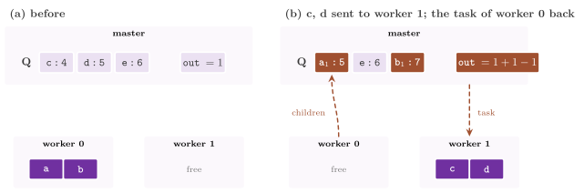
Proposition 13.17 (The end of the farm).
In Algorithm 13.9 each open node is either in Q or in a task that is
out at a worker, and out is the number of such tasks. Hence, the test
at line 5 is exact: the master returns only when each task is back and
either no node is open, or a limit is reached, or (through line 11) no
open node can improve the incumbent.
Proof. We observe that only the master changes Q and out. It moves
nodes from Q to a task and raises out (lines 12 and 13), and it lowers
out when a task comes back, pushing its children (lines 6 and 7). A
worker changes only the nodes of its task, replacing each node by the
children that survive PROCESS and keeping the dive within the task. When
out = 0 no task is out, and Q holds all the open nodes. \(\square\)
The master also never waits for nothing: if the evaluations terminate,
the farm ends. Indeed, a task out comes back in finite time, since its
worker processes at most batch nodes and their dives, each of which
ends at a leaf by (A4); and after each DISPATCH either out \(> 0\), or Q
is empty, or a limit is reached, since DISPATCH sends a task whenever
out \(< p\), Q is not empty and no limit is reached, unless it empties
Q at line 11. Hence the receive of line 6 always has a task to wait
for, each node is processed once, and the tree is finite.
In the farm the order of extraction is that of the selection, and the master only moves nodes; hence, the farm suits an evaluation that is "expensive" w.r.t. the transfer of a node. The batch of a task trades the messages for evaluations. The nodes of a task are extracted together, and the children of the first of them cannot overtake the others; a batch of 1 is therefore the one for an expensive evaluation, while the default of the parallel options, 16 nodes, amortizes the messages when the evaluation is "cheap". Also, the tasks are recycled through a free list of the master, and the farm runs \(p + 1\) threads, the master on the first CPU of the affinity mask when the workers are pinned. The dispatch is lines 8 to 13 of Algorithm 13.9, in which each task also carries the least open bound of the moment of its dispatch, the bound bl of the DIVE of its worker.
The deterministic rounds¶
The rounds (DeterministicBranchAndBound,
DeterministicBranchAndBound.h:125) make
the outcome independent of the timing of the workers, as the deterministic mode
of FiberSCIP [18] does, so that a run can be
repeated exactly (e.g., for the experiments of a paper, or to find a bug). At
each round the \(r\) best open nodes are extracted from one queue
(\(r\) = round, or \(p\) if 0), and the worker \(i\) processes the nodes
\(i, i + p, i + 2p, \ldots\) of the round against the incumbent \(z_0\) of
the start of the round. When all of them are done, one worker merges
the outcomes in the order of the nodes of the round and extracts the
next round, while the others wait at a barrier.
Algorithm 13.10 (The deterministic rounds).
 1  procedure DETERMINISTIC(R)
 2     Q ← R;  z ← the given incumbent, or ∞;  N ← ()
 3     in parallel, on each worker i = 0, ..., p − 1 do
 4        loop
 5           barrier, at which one worker runs NEXTROUND()
 6           if done then return
 7           for j = i, i + p, i + 2p, ... while j < |N| do
 8              (K_j, v_j) ← PROCESS(N_j) against z₀, v_j being the best
                   feasible value of N_j below z₀, if any
 9  procedure NEXTROUND()
10     for j = 0, ..., |N| − 1 do                  ▷ in the order of N
11        if v_j < z then z ← v_j;  N_j is the node of z
12        for each m ∈ K_j do
13           if PRUNABLE(β(m)) then m is a leaf (pruned) else push m in Q
14     if a limit is reached, Q = ∅ or PRUNABLE(the least bound of Q) then
15        done ← true;  return
16     N ← the first min(r, evaluations left) nodes of Q, removed
17     z₀ ← z
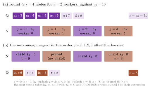
Theorem 13.18 (Determinism of the rounds).
Assume that no time limit is set, and that the evaluator of each worker
returns, for a node and an incumbent given by cutoff, an outcome that
depends only on them. Then the nodes evaluated, the incumbent value, its
node, the bound and the counters other than the evaluations of each
worker and the time are functions of the problem, of \(R\), of the options and of
\(r\), and depend neither on the timing nor on the number \(p\) of the
workers. If the outcome of the evaluator of worker \(i\) also depends on
the nodes that \(i\) evaluated before, the same holds with \(p\) among the
arguments. The node limit is exact.
Proof. We show by induction on the rounds that the state at the
barrier (the content of Q with the numbers of their pushes, \(z\) and its
node, the leaves and the counters) is such a function. At the start it
is fixed by \(R\) and the options. Given the state, NEXTROUND extracts
\(N\) by the order of the queue, which depends only on the keys and the
numbers of the pushes, and sets \(z_0\). Each outcome \((K_j, v_j)\) is
computed by PROCESS on \(N_j\) with the incumbent \(z_0\): the function
inc() that the workers pass returns the snapshot of the round, and
improve records the best value of the node without touching \(z\).
Hence, the outcome is a function of \(N_j\) and \(z_0\) under the first
assumption. Under the second one it is a function of \(N_j\), \(z_0\), \(p\)
and the earlier rounds, since the nodes of worker \(i\) are those of
index \(i \bmod p\). The merge then runs on one thread in the order of
\(j\). Finally, the last round is shortened to the evaluations left
(line 16), and a round never stops in the middle; thus the node limit
is met exactly. \(\square\)
We remark that the history of a worker depends on \(p\), as the proof
shows; hence, the independence of \(p\) needs an evaluation that depends
on the node (and on \(z_0\)) only, as that of the knapsack does, and a
history-dependent evaluator gives only the weaker property. Indeed, the
test bb-det-thread checks that the status, the value, the node, the
bound and the counters of the evaluated, generated and pruned nodes are
the same with 1, 2, 3 and 8 workers and at each repetition, also when a
node limit stops the search. The test bb-cutoff checks that the
value, the bound and the numbers of the evaluated and of the infeasible
nodes are the same with workers that fence the nodes by the incumbent
given by cutoff. The time limit, checked between the rounds,
makes the end depend on the timing.
The price is the wait of each round for its slowest node, which is
usually "small" when the evaluation dominates and its time varies little
among the nodes, and an incumbent that may be one round old (which may
cost somewhat more evaluations). Also, no dive is taken, and the
plunging selection extracts the nodes by their bound. In the code the
barrier is a std::barrier whose completion function is NEXTROUND; the
merge thus runs on one of the workers (the standard does not say which;
in practice the last to arrive) while the others are blocked.
Furthermore, the slots of a round, each with its node, its
children, its best value, its counters and its leaves, are reused from
round to round. An exception thrown by an evaluation is kept, and thrown
again by the search after the workers have stopped. The work of a worker
in a round is line 8 of Algorithm 13.10, with the function inc() of
PROCESS returning \(z_0\) and the function improve keeping in the slot
the best value below \(z_0\); the merge is lines 10 to 13, in the order of
the slots, where the counters of each slot are added to those of the
search, so that they do not depend on which worker processed the slot.
It remains to show that the rounds are correct and end.
Proposition 13.19 (The end of the rounds).
Under (A1) to (A4) and with \(\tau_r \le 1\), (i) at each barrier, after
NEXTROUND, every \(x \in X(R)\) with \(v(x) < \theta(z)\) is in the subset
of a node of Q or of the new round \(N\); (ii) when NEXTROUND sets done
with no limit reached, the value satisfies Theorem 13.5
and the bound Theorem 13.6; (iii) if the evaluations
terminate, the search ends after finitely many rounds.
Proof. (i) We argue by induction on the rounds. The slots of a round
are the nodes removed from Q at line 16, and each of them is processed
exactly once, by the worker \(j \bmod p\). PROCESS prunes by \(z_0\), a past
value of \(z\), which is safe by Lemma 13.12, and the value
found by a slot is offered to \(z\) at line 11, before the end test, so
that a node with no child is covered as in Lemma 13.4.
After the barrier each slot has been processed, and line 13 puts each
child in Q or makes it a leaf by the current \(z\); hence, at line 14, the
open nodes are those of Q, and the claim follows from the proof of
Lemma 13.4 applied to each slot. (ii) At line 14 no node
is held by a worker and none is in a slot, since the end is decided by
one thread while the others wait at the barrier; hence done is set
only when Q is empty or no node of Q can improve \(z\), which are the
situations of Theorem 13.13. (iii) A round processes at
least one node, since \(r \ge 1\) at line 16 (with a node limit,
NEXTROUND stops at line 14 as soon as the evaluations reach it), and
each node is processed once in a finite tree; a round ends when its at
most \(\lceil r / p \rceil\) processings per worker end. \(\square\)
13.9 One pool per worker¶
The distributed queues¶
In the distributed queues (DistributedBranchAndBound,
ParallelBranchAndBound.h:638) each worker has
a queue \(Q_i\) and sends each child, in batches, to the worker that owns it, as
HDA\(^*\) does with the states of A\(^*\) (Chapter
9). Its owner is \(\mathrm{hash}(m) \bmod p\) if
the problem gives a hash of its nodes, and a random worker otherwise. Since a
tree has no duplicates, the owner only balances the load, and a uniform hash is
perhaps the most suitable distribution; the distributions of HDA\(^*\) that keep
related states on the same worker (abstraction, abstract Zobrist hashing) have
little to gain here. In the Doxygen comment of
ParallelBranchAndBound.h the pseudocode follows
that of the shared queue, as its lines 28 to 45; here its lines are numbered
from 1.
Algorithm 13.11 (The distributed queues).
 1  procedure DISTRIBUTED(R)  ▷ a queue Q_i per worker, nodes to the owners
 2     put each node of R in the queue of its owner
 3     in parallel, on each worker i = 0, ..., p − 1 do
 4        d ← nil
 5        while the search is not over do
 6           push the nodes received in Q_i
 7           if d ≠ nil then n ← d;  d ← nil
 8           else if Q_i ≠ ∅ and not PRUNABLE(the least bound of Q_i) then
 9              n ← the first node of Q_i, removed
10           else
11              the nodes of Q_i are leaves (pruned);  Q_i ← ∅
12              send all the outboxes;  wait for mail or the end; continue
13           if a limit is reached then n is a leaf (open); stop all; return
14           K ← PROCESS(n);  d ← DIVE(K)
15           for each m ∈ K but d do
16              j ← hash(m) mod p, or a random worker without hash(m)
17              if j = i then push m in Q_i else send m to j
18           every k evaluations, send the outboxes not yet full
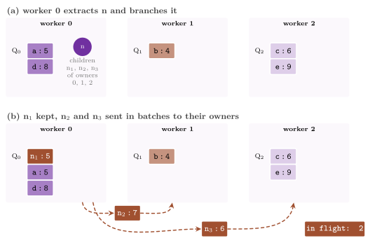
Proposition 13.20 (The end of the distributed queues). Algorithm 13.11 ends only when no worker holds a node and no node is in flight, with each queue empty (a queue whose least bound cannot improve the incumbent having been emptied into leaves at line 11); if the evaluations terminate, it ends.
Proof. As we said, the wider open set is made of the queues, the dives
and the nodes in the outboxes and in flight. A worker reaches the test
of the end (line 12) only with no dive and an empty queue, after sending
all its outboxes. The test is that of the mailbox (quiescent()), the
deficit counting of Definition 9.6,
whose hypotheses hold here: a worker sends only while it has work (at
line 17, or when the mailbox flushes its outboxes before it becomes
passive) and becomes active again only by draining a message (line 6).
By Lemma 9.7 the mailbox reports the
end only when no worker is active and no message exists, i.e., when
each worker is at line 12 with no dive and an empty queue and each
node sent has been received; at that moment the wider open set is
empty. Conversely, while a node exists in the wider set, some worker
holds it or will receive it, and processes it in finite time; since
each node is processed once and the tree is finite, the end comes, and
by part (iii) of the lemma all the workers then read it. After a stop
at a limit the mailbox reports the end to all the workers at once, and the
nodes left in the queues, in the dives, in the outboxes and in the
channels are collected as open leaves once the workers have returned
(leftovers()), so that the bound covers them. \(\square\)
The batches are of 16 nodes by default, and the outboxes are flushed at
each evaluation (flush_period = 1), since an evaluation is usually
"expensive" and a node that waits in an outbox delays its owner. The
nodes a search starts from go to their owners, or to the worker \(i \bmod
p\) for the \(i\)-th of them when the problem gives no hash. Without a
hash, the owners come from a generator per worker, seeded by seed plus
the index of the worker. Note that, since a worker extracts the best
node of its queue only, it may evaluate nodes "far" worse than the
best open one before an incumbent prunes them, and how many depends on
when the incumbent is found, i.e., on the timing. Plunging, whose dives
reach a leaf early, tends to keep them close to those of the sequential
search. The choice of the owner is lines 15 to 17 of Algorithm 13.11,
the random owner being drawn by a generator of 64 bits of each worker.
The distributed queues over MPI¶
Over MPI (MPIBranchAndBoundSearch,
MPIBranchAndBound.h:168) the same scheme runs with
one process per worker, and the nodes travel as bytes, written by serialize()
and read by deserialize() (a trivially copyable node needs neither). Each
process has its queue and a copy of the incumbent value. A process that
improves it sends the value to all the others, while the node of the incumbent
stays with the process that found it until the end, when the process of the
least value sends it to all.
Algorithm 13.12 (The distributed queues over MPI).
 1  procedure MPI-B&B(R_i) on the process i       ▷ R_i: its own nodes
 2     Q_i ← R_i;  d ← nil
 3     loop
 4        for each message m received do
 5           if m is a batch of nodes then push them in Q_i
 6           else if m is an incumbent z' then z ← min(z, z')
 7           else if m is a stop then stop evaluating
 8        if not stopped and (d ≠ nil or not PRUNABLE(βmin(Q_i))) then
 9           n ← d, or the first node of Q_i, removed;  d ← nil
10           K ← PROCESS(n), a value v < z sending v to all the others
11           d ← DIVE(K)
12           for each m ∈ K but d do
13              j ← hash(m) mod p, or a random process without hash(m)
14              if j = i then push m in Q_i else send m to j
15           every k evaluations, send the outboxes not yet full
16           if the share of the node limit or the time limit is reached
                then stop all the processes
17        else send all the outboxes
18        if the mailbox detects the end then break
19     the nodes still travelling, after a stop, are put in Q_i
20     the process of the least z sends its node to all
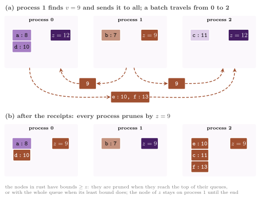
Proposition 13.21 (Correctness and end over MPI). The value and the bound returned by Algorithm 13.12 satisfy Theorems 13.5 and 13.6 when no limit stops it, and the bound satisfies Theorem 13.6 in any case; the search ends when no process has a node that can improve its incumbent and no message is in flight.
Proof. We first note that the value \(z\) of a process is at any moment at least the least value found by all, which plays the part of the shared incumbent of Theorem 13.13. Indeed, it is the initial value or a value received, each value sent is feasible, and a process that prunes by a (possibly larger) value prunes less, as in Lemma 13.12. The end is detected by the four-counter method of Mattern [11] in the mailbox of MPI (proved sound in Theorem 9.18), which a process joins (line 18) only when it has no node to evaluate and has sent all its outboxes. The method counts each message, the incumbents included, and reports the end only when all the processes are passive and each message sent has been received. At that moment each process has turned its queue into leaves by its incumbent (line 8), which is at least the least value found, and no node travels; the wider open set is then empty, and Theorem 13.13 applies. After a stop at a limit, the nodes still in flight are received as open leaves (line 19), and the bound covers them. \(\square\)
The node limit \(L\) is split among the processes, each stopping at
\(\lceil L / p \rceil\) evaluations, and a process that reaches its share,
or the time limit, stops the evaluations of all. Each process returns
the same value, node and bound (an all-gather of the values picks the
process of the least value, the least rank on ties, which broadcasts
its node). Each keeps, however, the leaves
it owns, and the reoptimization of §13.11 then starts each
process from them, with no transfer. All sends are non-blocking. MPI
must be initialized by the caller, with at least MPI_THREAD_FUNNELED
if the problem uses threads. The broadcast of an improvement is line 10
of Algorithm 13.12: a value \(v\) below the local \(z\) becomes the local
incumbent, with its node, and is sent, as its bytes, to each other
process with a tag of its own.
The work stealing¶
In the work stealing (StealingBranchAndBound,
StealingBranchAndBound.h:117), after Blumofe
and Leiserson [20], each worker pushes the children
it generates in its queue and extracts the best node of that queue. A
worker whose queue is empty steals about half of the queue of another
one, drawn at random, the half that leaves the victim its best node (cf.
the steal-half queues of Hendler and Shavit
[36]). A worker then typically stays in its
part of the tree. This pays off when moving its evaluator to a distant
node costs (e.g., when the evaluator applies and undoes the branchings
along the path from the root), while the nodes of the distributed queues
land on any worker.
Algorithm 13.13 (The work stealing).
 1  procedure STEALING(R)
 2     the k-th node of R in Q_(k mod p)
 3     in parallel, on each worker i = 0, ..., p − 1 do
 4        d ← nil
 5        loop
 6           if d ≠ nil then n ← d;  d ← nil
 7           else n ← NEXT(i);  if n = nil then return
 8           if a limit is reached then
 9              n is a leaf (open);  stop all the workers;  return
10           K ← PROCESS(n)
11           d ← DIVE(K);  push the nodes of K but d in Q_i
12  procedure NEXT(i)
13     if Q_i ≠ ∅ and PRUNABLE(the least bound of Q_i) then
14        the nodes of Q_i are leaves (pruned);  Q_i ← ∅
15     if Q_i ≠ ∅ then return the first node of Q_i, removed
16     loop
17        if stopped, or no worker holds a node or works on one, return nil
18        v ← a worker ≠ i at random
19        if Q_v holds two nodes at least then
20           move about half of them, but the first, to Q_i
21           if some were moved, return the first node of Q_i, removed
22        wait a little
The queues are the stealable priority queues of the default data structures of the library, whose owner extracts its nodes in the exact order of the selection and with no lock. Each queue keeps its nodes in two 4-ary heaps, \(H_0\) and \(H_1\), which no other thread reads. A push goes into the smaller of the two, and hence the nodes pushed one after the other (e.g., the children of a node) are dealt to the two heaps in turn; a pop takes the better of their two least nodes. A thief that finds no node to claim raises a flag of the queue of the victim. The owner reads it at its next operation, and moves the heap whose least node is not the least of the queue into the offer of the queue, an atomic pointer, which a thief claims by an exchange with null (Figure 13.12). Note that the owner keeps its least node. Until a thief claims the offer, its nodes still belong to the owner: a pop whose least local key is not less than the least key of the offer takes the offer back by the same exchange, and whoever of the two exchanges first gets it all. Hence, the common case of the owner, a push or a pop with no thief waiting, costs no read-modify-write and no fence. A steal costs the thief two exchanges at most, and the owner the store of a pointer (or the time to deal its nodes again to two heaps of equal size, when they differ in size by more than a factor of 4). The price is that a thief waits for the next operation of the victim, i.e., at most the processing of one node.
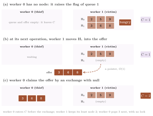
Proposition 13.22 (The end of the work stealing). Let \(C\) be the number of the workers that hold a node or work on one, plus the thieves that are trying to claim an offer. A worker leaves \(C\) when its pop finds its queue and its offer empty, and a thief enters \(C\) before the exchange that claims an offer and leaves it if the exchange fails. Then \(C = 0\) only when no node is open, and the test at line 17, which returns nil when \(C = 0\), is exact; if the evaluations terminate, each worker returns.
Proof. We claim that a node is at any moment in a heap of its owner, in an offer (which belongs to the owner until claimed), in the hands of a thief between its exchange and its first pop, or held by a worker. In the first two cases the owner is counted in \(C\), since it left \(C\) only after finding its heaps and its offer empty, and it re-enters only by a steal. In the third case the thief entered \(C\) before its exchange, and in the fourth the worker is counted. Hence a node exists only if \(C > 0\). A worker loops at lines 16 to 22 only while \(C > 0\), i.e., while some worker holds or works on a node. That worker processes it in finite time, and then pushes children (which a thief can claim after the next operation of the owner) or drops it; the tree is finite. \(\square\)
The price of the scheme is a selection that is best-first within each
queue only, and hence an order of extraction that may be farther from
the sequential one than that of the shared queue. Also, the nodes have
to be copyable with moves that do not throw, since a steal moves them to
the thief, and the counter of the nodes sent in BBStats holds the
steals. The extraction of a worker (lines 12 to 15 of Algorithm 13.13)
drops its queue at once when its least bound, which counts the offer
not yet claimed, cannot improve the incumbent.
The SelfSplit¶
The SelfSplit of Fischetti, Monaci and Salvagnin
[19] (SelfSplitBranchAndBound,
SelfSplitBranchAndBound.h:130) gives a B&B
whose workers communicate only at the end. The tree is first explored
sequentially (the sampling), by the evaluator of the worker 0 and without
plunging, until the open nodes are \(\sigma p\) (\(\sigma\) being split, 4 by
default) or the tree is solved. Then, with split_dive (the default),
the same evaluator dives from a copy of the first open node to a leaf,
taking at each level the child of least estimate (of least bound, if
the problem gives no estimate). Finally the \(k\)-th open node, in the
order of the selection, goes to the worker \(k \bmod p\). Each worker
searches its subtrees sequentially (by BranchAndBoundSearch) with its
evaluator, an incumbent starting from that of the sampling, and its
share of the node limit and of the time left; the incumbents, the
bounds and the leaves of the workers are merged in the order of the
workers.
Algorithm 13.14 (The SelfSplit).
 1  procedure SELFSPLIT(R)
 2     Q ← R;  z ← the given incumbent, or ∞     ▷ the sampling, by worker 0
 3     while p > 1 and Q ≠ ∅ and |Q| < σ p do
 4        if a limit is reached then break
 5        if PRUNABLE(the least bound of Q) then
 6           the nodes of Q are leaves (pruned);  Q ← ∅;  break
 7        n ← the first node of Q, removed;  Q ← Q ∪ PROCESS(n)
 8     if p > 1, split_dive and Q ≠ ∅ then         ▷ the dive, by worker 0
 9        n ← a copy of the first node of Q
10        while n ≠ nil and no limit is reached do
11           n ← the child of PROCESS(n) of least estimate, or nil
12     for k = 0, 1, ..., while Q ≠ ∅ do           ▷ the split
13        add the first node of Q, removed, to R_(k mod p)
14     in parallel, on each worker i = 0, ..., p − 1 do
15        S_i ← B&B(R_i) on the evaluator of i, from the incumbent z, with
             its share of the node limit and the time left, pruning also
             by the incumbent of all the workers if split_shared
16     z ← min(z, the values of the S_i), the node of the least i on ties
17     return z, its node, the leaves of the sampling and of the S_i, and
          the least of their bounds
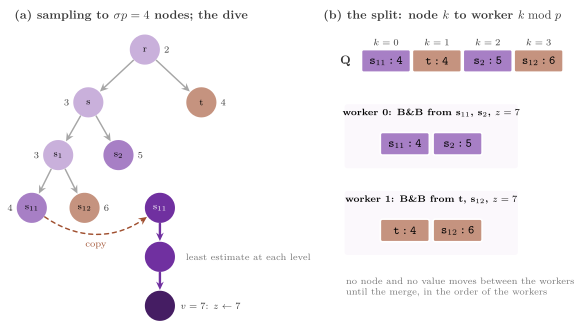
Theorem 13.23 (The SelfSplit). Under (A1)
to (A4) and with \(\tau_r \le 1\), (i) when no limit stops it, the value
returned by Algorithm 13.14 satisfies Theorem 13.5, and its
bound satisfies Theorem 13.6 in any case. (ii) Without
split_shared and without a time limit, its outcome depends only on
the problem, \(R\), the options, \(\sigma\) and \(p\), provided that the
evaluation of a node by a worker depends only on the node, the
incumbent given by cutoff and the nodes evaluated by that worker
before. (iii) If the evaluations terminate, the search ends, its end
being the return of the last worker.
Proof. (i) We observe that the sampling is Algorithm 13.3 stopped
early. Hence, by Lemma 13.4, each element of \(X(R)\) below
the threshold of its incumbent \(z_s\) is in an open node at its end, and
its leaves bound the rest. As for the dive, it works on a copy and
records no leaf; it may only lower \(z_s\), by a value found. Then the
split partitions the open nodes among the \(R_i\), and each worker is a
sequential B&B from \(R_i\) with the initial value \(z_s\). Let \(z = \min_i
z_i\); the value \(z_i \le z_s\) of the worker \(i\) satisfies \(\min \{ v(x)
: x \in X(R_i) \} \ge \theta(z_i) \ge \theta(z)\) by Theorem
13.5 and Lemma 13.3. With split_shared the
worker \(i\) prunes by the least \(c_i\) of \(z_i\) and of the values found
by the others, and the same argument gives the bound
\(\theta(c_i) \ge \theta(z)\), since \(c_i \ge z\). The elements that the
sampling left below \(\theta(z_s)\) are in some \(X(R_i)\), and those of its
leaves are not below \(\theta(z_s) \ge \theta(z)\); hence \(z^*_R \ge
\theta(z)\). The bound is the least of the bounds of the sampling and of
the workers, each valid by Theorem 13.6 for the region it
covers, and these regions cover \(X(R)\). (ii) The sampling and the dive
are sequential, and the split depends only on the order of the queue and
on \(p\). Worker \(i\) receives \(R_i\), \(z_s\) and its share of the limit, all
fixed, and runs with no exchange, with its evaluator; the merge goes in the
order of the workers. (iii) The sampling stops when its queue holds
\(\sigma p\) nodes, or earlier, and processes each node once in a finite
tree; the dive ends at a leaf by (A4); each worker runs Algorithm 13.3,
which ends by Theorem 13.5; and the search waits for all
the workers to return before the merge, so that no node is open
anywhere when it merges. \(\square\)
The proof also shows why the dive matters. A best-first sampling seldom
reaches a leaf, and without an incumbent a worker whose subtrees do not
hold the optimum evaluates each node of them whose bound is better than
the best value in them, since no incumbent prunes them. Yet, the dive
gives each worker the incumbent of one leaf, at the cost of the "few"
nodes of the dive, which the worker whose subtree holds them evaluates
again (both evaluations are counted). With split_shared the workers
also prune by the best incumbent of all of them, which each reads at
each extraction through shared_incumbent. Even so, the value is still the
optimum, since the shared value is a value found (cf. Lemma
13.12), while the nodes evaluated, and the node of the
optimum among equal values, depend on the timing. With one worker there
is nothing to split: the root goes to it with neither the sampling nor
the dive, and the nodes evaluated are those of the sequential search.
The test bb-split-thread checks this, and that the outcome is the same
at each repetition, with a split of 1 and 4 nodes per worker and with
and without the dive.
In the library the sampling is done once, by the worker 0, rather than
by each worker as in the original scheme, since the workers share the
memory and can read its open nodes. Over MPI, where a node would
otherwise travel as bytes, each process would repeat it, as Fischetti,
Monaci and Salvagnin do. Its price is a load that is
balanced only as far as the subtrees of the split are, and (without
split_shared) an incumbent found by a worker that does not prune the
nodes of the others. The split is lines 12 and 13 of Algorithm 13.14:
with \(L'\) the evaluations left by the sampling, the worker \(i\) receives
the share \(\lfloor L' / p \rfloor + 1\) if \(i < L' \bmod p\) and
\(\lfloor L' / p \rfloor\) otherwise, so that the shares sum to \(L'\), and
a node whose worker has a share of 0 becomes an open leaf. The dive is
lines 8 to 11, taking the first of the children of least estimate;
its leaves go to a record of Algorithm 13.4 that keeps nothing, since
the open nodes of the sampling still cover them.
13.10 The schemes compared and chosen by name¶
Table 13.1 gathers, for each scheme, where the open nodes are, how the end is detected and on what the outcome depends. Here "the timing" means that two runs with the same data may evaluate different nodes, and return a different node among those of equal value. The value is in any case within the tolerance of the optimum in each run that no limit stops.
Table 13.1. The B&B searches of the library: where the open nodes
are, how the end is detected (the condition of the proposition of each
scheme), and on what the outcome depends besides the problem and the
options; for the rounds, \(p\) matters only with an evaluator that
depends on the history of its worker (Theorem 13.18), and
the SelfSplit depends on the timing with split_shared.
| Scheme | Open nodes | End | Depends on |
|---|---|---|---|
| sequential | one queue | Q empty, or line 6 | nothing |
| shared | one queue, a lock | Q empty, busy \(= 0\) | the timing |
| multiqueue | \(2p\) queues, a lock each | \(m = 0\) | the timing |
| farm | the queue of the master | out \(= 0\) | the timing |
| deterministic | one queue, by rounds | between rounds | \(r\) (and \(p\)) |
| distributed | a queue per worker | message counts | the timing |
| MPI | a queue per process | Mattern's counters | the timing |
| stealing | a queue per worker | \(C = 0\) | the timing |
| selfsplit | a queue per worker | at each worker | \(\sigma\), \(p\) |
| skeletons | stacks, a pool per worker | \(\pi = 0\) | the timing |
| ordered | stacks, one list of tasks | the list is taken | the timing |
| hubs (MPI) | a queue per process | Mattern's counters | the timing |
| intervals | an interval per worker | active \(= 0\) |
the timing |
We expect the choice among the schemes to depend on the cost of an
evaluation w.r.t. that of moving a node, and on the variance of that
cost among the nodes, which only a measurement on the instances of
interest can settle. The shared queue and the farm keep the order of the
selection, at the price of a lock or of a master, and the MultiQueue
removes the lock at the price of the order. The distributed queues and
the work stealing remove the common pool, the latter keeping each worker
in its part of the tree. Finally, the rounds and the SelfSplit perhaps
give up some speed for an outcome that does not depend on the timing.
All the schemes but the farm and the search over MPI, which build their
workers and their channels themselves, can be chosen at run time by a
value of the enumeration BBScheme, or by its name, read, e.g., from
a file of parameters. The enumeration is
enum class BBScheme {
 sequential ,      ///< one worker [see BranchAndBoundSearch]
 shared ,          ///< one shared queue [see SharedBranchAndBound]
 distributed ,     ///< a queue per worker [see DistributedBranchAndBound]
 deterministic ,   ///< synchronous rounds [see DeterministicBranchAndBound]
 selfsplit ,       ///< a split of a sampling [see SelfSplitBranchAndBound]
 stealing ,        ///< work stealing [see StealingBranchAndBound]
 multiqueue ,      ///< a MultiQueue [see MultiQueueBranchAndBound]
 depth_bounded ,   ///< depth-first, spawning above a depth [see BBRule]
 budget ,          ///< depth-first, spawning after a budget [see BBRule]
 stack_stealing ,  ///< depth-first, stealing from the stacks [see BBRule]
 ordered           ///< depth-first, ordered tasks [see BBRule]
 };
and the functions of BranchAndBoundScheme.h are
declared as follows (without their bodies; the template head of
parallel_branch_and_bound() has the problem type P and, as its
second parameter, the executor):
[[nodiscard]] inline std::string_view bb_scheme_name( BBScheme s );
[[nodiscard]] inline BBScheme bb_scheme( std::string_view name );
[[nodiscard]] BBSolution< typename P::node_type , bb_value_t< P > >
parallel_branch_and_bound( const P & problem , BBScheme s ,
                           const BasicParallelBBOptions< bb_value_t< P > > &
                             o = {} ,
                           std::optional< std::vector< BBLeaf<
                             typename P::node_type , bb_value_t< P > > > >
                             seeds = std::nullopt );
Thus, a program built on the library gets each new scheme with no change
of its code. The following example, from the case manual of the
tester, which the build compiles and runs (ctest -R PBeFS.manual),
solves a knapsack kp of 50 items by the sequential search s, with
the options o, and by the scheme sch read from its name, with the
parallel options po and 4 workers, and shows that an unknown name is
refused; the case then checks both solutions against the dynamic
program.
// a random 0-1 knapsack of 50 items, of class 0
const Knapsack kp = Knapsack::random( 0 , 50 , 1000 , 1 );
BBOptions o;
o.selection = Selection::best_first;     // the least bound first
const auto s = branch_and_bound( kp , o );
// s.status, s.value and the incumbent node s.node
ParallelBBOptions po;
po.threads = 4;
const BBScheme sch = bb_scheme( "stealing" );   // a name, e.g., from a file
const auto r = parallel_branch_and_bound( kp , sch , po );
bool refused = false;
try {
 ( void ) bb_scheme( "nonesuch" );
 }
catch( const std::invalid_argument & ) {     // not the name of a scheme
 refused = true;
 }
The names are sequential, shared, distributed,
deterministic, selfsplit, stealing, multiqueue, and the four rules
of the skeletons of §13.14, depthbounded, budget,
stackstealing and ordered (an unknown name throws
std::invalid_argument, and so does multiqueue with values that are
not atomic with no lock). When the options list the settings of a race
(§13.15), parallel_branch_and_bound() runs the race first
and goes on by the scheme of the call from the leaves of the winner. The
farm, the search over MPI, the hubs of §13.17 and the
intervals of §13.18 are not among the named schemes, and
they are used by their classes, FarmBranchAndBound< P , Executor >( problem , options ) and
MPIBranchAndBoundSearch< P >( problem , options , comm ),
MPIHubBranchAndBoundSearch< P >( problem , options , hub , comm ) and
IntervalBranchAndBound< P , Executor >( problem , options ), whose
solve() returns the solution. The executor, i.e., the pool of C++
threads, OpenMP or FastFlow, is the second template parameter of each
parallel search on threads. Also, set_executor() gives a search an
executor that outlives it (without one, each search builds a pool).
13.11 Reoptimization¶
When the data of the problem change in a way that leaves the branching
valid (e.g., a restriction of the feasible region, or a change of the
objective that the nodes do not store), the tree explored by a previous
search need not be built again. Its leaves cover the subtrees of the
nodes that the search started from, and a new search can start from
them. With keep_frontier, the BBSolution holds these leaves, each
with its bound (in the sense of the problem), its depth and its kind.
The overload solve( seeds ) of each search (and
branch_and_bound( p , seeds , options )) starts from any set of such
nodes instead of the root, each of them being an open node that is
evaluated only when it is extracted. Figure 13.14 shows
the simplest use: a search stopped by a node limit is resumed from its
open leaves, together with its incumbent.
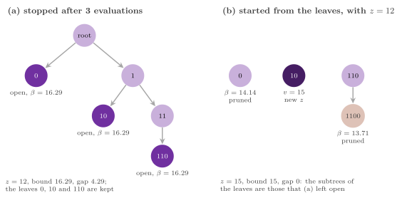
Proposition 13.24 (Reoptimization). Let
\(L\) be the leaves of a search from \(R\) with keep_frontier. (i) Every
element of \(X(R)\) belongs to \(X(l)\) for some \(l \in L\). (ii) If the
problem changes to \(X'\) and \(v'\), with (A2) to (A4) holding for it,
with the children generated by the previous search still covering the
new subset of their parent (A1), with the subsets of the nodes
\(X'(n) \subseteq X(n)\), and with
\(v' = v\), then a search from the non-infeasible leaves of \(L\), with
their bounds, solves the new problem over \(X'(R)\) in the sense of
Theorems 13.5 and 13.6. (iii) If instead
\(X'(n) \supseteq X(n)\), or \(v' \ne v\), the same holds when each leaf,
the infeasible ones included, is given back with an unknown bound
(\(-\infty\) in the minimization), or with a bound that the caller knows
to be valid for the new problem.
Proof. Part (i) is the covering shown in the proof of Theorem 13.6. (ii) The bound of a leaf was a bound of \(X(l)\) for \(v\), and hence of \(X'(l) \subseteq X(l)\); an infeasible leaf has \(X'(l) \subseteq X(l) = \emptyset\). Hence, the seeds cover \(X'(R)\) with valid bounds, and the proofs of Lemma 13.4 and of the theorems apply with the seeds in place of \(R\); the covering of \(X'(R)\) by the seeds follows, as in (i), from (A1) applied to the nodes that the previous search branched. (iii) An unknown bound is valid for any problem, and the seeds cover \(X'(R)\) by the same argument, since (A1) for the new subsets is again assumed of the children that the previous search generated (all the leaves, the infeasible ones included, being given back). \(\square\)
Which leaves are given back, and with which bounds, is left to the
caller, since only the caller
knows what has changed. After a restriction of the region the bounds of
the pruned leaves remain valid, and the infeasible leaves need not be
explored again. After an enlargement the infeasible leaves have to be
given back with an unknown bound. After a change of the objective all of
them have to be given back with an unknown bound, unless the old ones
can be corrected (say, by a bound on the change of the objective over
the node). A search stopped by a limit is resumed by giving back its
open leaves together with its incumbent, as in Figure
13.14. The bound of the new BBSolution is that of the
subtrees of the seeds, and the caller combines it with the bounds of the
leaves that it leaves out. The test bb and the parallel tests check
three uses on the knapsack. First, the leaves of a search carried out to
the end bound the optimum and solve the knapsack of three quarters of
the capacity. Second, with explicit_children, the leaves of the
smaller knapsack, the infeasible ones among them, solve the original one
again (without explicit_children the child that takes an item that
did not fit is never generated, and (A1) fails for the larger
capacity). Third, the open leaves of a search stopped by a node limit end
it.
In the parallel searches each worker collects its leaves, which are
merged at the end, and the seeds go to their owners as the children do.
Over MPI each process keeps the leaves that it owns and starts from its
seeds, which avoids sending them across the processes. We remark that
in a tree where every inner node has two children the leaves are one
more than the inner nodes, and therefore keeping them may take much
more memory than the open nodes; hence, keep_frontier is off by
default.
13.12 The interface for a branch-and-bound solver¶
A B&B solver built on a modeling system (e.g., for Mixed-Integer Linear
Programs) would provide a problem whose node_type is the list of the
branching decisions from the root, e.g., the bounds changed on the
variables, which is "small" and hence "cheap" to copy and to send. Its
make_worker( i ) would return an object holding a copy of the model
and of the solver of the relaxation. The evaluate of a worker applies
the decisions of the node to its model (possibly undoing only those
that differ from the previous node, which makes a dive "cheap") and
solves the relaxation. It returns the value of the relaxation as the
bound, its infeasibility, and the same value as a feasible one if the
solution is integral. Its branch chooses a fractional variable in the
solution stored in the node, and gives the two children with the bound
of the parent as their estimate. Its cutoff( z ) should keep the
incumbent value (and pass it to the solver of the relaxation as an
objective limit), and its evaluate should return as feasible only the
values found at the node, keeping the solution in the node;
then the outcome is that of the scheme it runs, whichever it is. In
particular, the deterministic rounds and the SelfSplit then give a
solver whose runs can be repeated exactly, under the conditions of
Theorem 13.18 and Theorem 13.23; a warm
start from the previous node of the worker satisfies them only in their
weaker form, in which the outcome depends on \(p\). Such a solver calls
parallel_branch_and_bound() with the name of a scheme read from its
parameters, as in §13.10, and reads the incumbent, its
node, the bound and the gap from the BBSolution. In the options it
gives the selection, the tolerances, the initial incumbent and the
callback, and for the parallel searches the number of workers, the
batch, the nodes of a round and those of the split. The test
bb-cutoff checks this interface with workers that fence the nodes by
the incumbent they receive.
13.13 Lazy children, indexed children and the modes¶
The sections from here to the end of the chapter treat the parts of the layer that extend the core of the previous sections: the children given one at a time and the modes of the search (this section), the depth-first skeletons (§13.14), the racing ramp-up (§13.15), the checkpoints (§13.16), the master, the hubs and the workers over MPI (§13.17), the work stealing of intervals of leaves (§13.18) and the example problems that exercise them (§13.19); their benchmark, notes and exercises are in §13.20, §13.21 and §13.22 with those of the core.
The children one at a time¶
The method branch( n , sink ) of §13.1 gives all the
children of a node at once, which suits the searches that keep a queue,
since each child that survives the test of line 26 of Algorithm 13.3 is
pushed anyway. A depth-first search, instead, visits the children of a node
one at a time and often abandons the rest of them, e.g., when the children
come by increasing estimate and the first one pruned makes the others
prunable too; building the children it never visits is then wasted work,
which in some problems (the cliques of §13.19 among them)
is most of the work of a branching. Hence, the evaluator may give the
method children( n ) in place of, or besides, branch( n , sink ): it
returns a cursor, a model of the concept BBCursor, whose next()
gives the next child of the evaluated node n with its estimate, as a
BBChild, or nothing when there is no more. The child and the cursor are the following
(BranchAndBound.h:208 and
BranchAndBound.h:332):
template< class Node , class V = double >
struct BBChild {
 Node node;          ///< the child
 V estimate;         ///< a bound of it that is cheap to compute
 };
template< class C , class N , class V = double >
concept BBCursor = requires( C & c ) {
 { c.next() } -> std::convertible_to< std::optional< BBChild< N , V > > >;
 };
The concept BBEvaluator of §13.1 accepts an evaluator that
gives either method, and two refinements of it name the evaluators that
give the optional ones (BranchAndBound.h:383
and BranchAndBound.h:392):
template< class W , class N , class V = double >
concept LazyBBEvaluator = BBEvaluator< W , N , V > &&
 requires( W & w , const N & cn ) {
  { w.children( cn ) } -> BBCursor< N , V >;
  };

/*- - - - - - - - - - - - - - - - - - - - - - - - - - - - - - - - - - - - -*/
/// an evaluator that gives the child k of a node [see BBEvaluator]

template< class W , class N , class V = double >
concept IndexedBBEvaluator = BBEvaluator< W , N , V > &&
 requires( W & w , const N & cn , std::size_t k ) {
  { w.child( cn , k ) }
   -> std::convertible_to< std::optional< BBChild< N , V > > >;
  };
A LazyBBEvaluator gives children( n ), and an IndexedBBEvaluator
gives child( n , k ), the child \(k\) (counted from 0) of n built
without the evaluation of n, or nothing if n has fewer children. The
latter is used by the searches that rebuild a node from the path of the
choices that lead to it (§13.14) or from its interval of
leaves (§13.18); it requires that the children of a node
come in an order that depends only on the node, and that child( n , k )
give the \(k\)-th of them in that order. When the problem has no
make_worker( i ), the problem itself is the evaluator of each worker,
and it gives each of these methods when it declares it.
Every problem runs on every search, whichever methods its evaluator
gives. The searches that take all the children at once call branch( n ,
sink ) when the evaluator has it, and otherwise read the cursor of
children( n ) to its end (detail::bb_branch()); conversely, the
skeletons of §13.14, which take the children one at a
time, use the cursor of children( n ) when the evaluator gives it, and
otherwise a cursor on a vector filled by branch( n , sink )
(detail::bb_children()). Only the skeletons draw a benefit from the
lazy children, since they are the only searches that stop reading a
cursor before its end; in the other searches a lazy evaluator builds all
the children as an eager one does. The cursor of a frame of a skeleton
may refer to its node, which does not move while the frame exists, as
the cursor of MaxClique does.
The option prune_level of BasicBBOptions states that the children of
every node come by their estimates, the best first, i.e., by
nondecreasing estimate in the minimization. Under this assumption, a child
pruned at its generation (line 26 of Algorithm 13.3) ends its siblings:
the search marks the rest of them as pruned without testing them, and a
skeleton never asks its cursor for them, so that they are never built
(unless keep_frontier asks for them as leaves, in which case they are
built, counted as generated and pruned, and recorded).
Proposition 13.25 (The children pruned by
level). Let the estimates \(e_1, e_2, \ldots\) of the children of each node
be nondecreasing in the order of the children, in the minimization, and
let \(\tau_r \le 1\). If the child \(m_j\) is pruned at its generation, then
every later child \(m_k\), \(k > j\), would be pruned at its generation too,
in each of the three modes defined below. Hence, with prune_level every
search of the library keeps the guarantees of its scheme, a sequential
search evaluates the same nodes and returns the same value and bound as
without it, and the counter generated of a skeleton is lowered by the
children it does not build.
Proof. Let \(z_j\) be the incumbent at the generation of \(m_j\) and \(z_k\)
that at the generation of \(m_k\); since the incumbent never increases
(Lemma 13.12), \(z_k \le z_j\). The bound of \(m_k\) is
\(\beta(m_k) = \max \{ \beta(n), e_k \} \ge \max \{ \beta(n), e_j \} =
\beta(m_j)\). In the mode optimize, \(\beta(m_j) \ge \theta(z_j) \ge
\theta(z_k)\) by Lemma 13.3, and therefore \(\beta(m_k) \ge
\theta(z_k)\). In the mode enumerate, \(\beta(m_j) = +\infty\), and then
so is \(\beta(m_k)\). In the mode decide, either the target was met by
\(z_j\), and then it is met by \(z_k \le z_j\), or \(\beta(m_j)\) exceeds the
target or is infinite, and then so does \(\beta(m_k)\). In each case the
test PRUNABLE of the mode is true for \(\beta(m_k)\). A child pruned at its
generation lowers only the bound low of the record of the leaves
(Algorithm 13.4) by its bound, which is at least the bound of the child
that started the cut; hence, low is unchanged as well. \(\square\)
The library does not check the assumption, and a problem whose children
do not come by their estimates gets a search that may miss its optimum
with prune_level. In the work stealing of intervals
(§13.18) each child is built by child( n , k ) on its
own, and the option has no effect there.
The modes¶
The mode of the options (BBMode,
BranchAndBound.h:183) says what the search looks
for:
enum class BBMode {
 optimize ,     ///< an optimal value
 decide ,       ///< a value within the target, stopping at the first one
 enumerate      ///< every node, counting the feasible ones
 };
In the mode optimize, the default, the search seeks an optimal value, as
in the previous sections. In the mode decide it seeks a feasible value
at least as good as the target of the options (any feasible value if no
target is given), and it stops as soon as one is found; this is the
decision problem of, e.g., the subgraph isomorphism of
§13.19. In the mode enumerate it visits the whole tree,
pruning only the infeasible nodes, and the counter solutions of
BBStats holds the number of the feasible values found, i.e., of the
feasible nodes of the tree, which is how the nodes of a tree of UTS or the
embeddings of a pattern graph are counted. (The counter solutions is
raised at each evaluation that gives a feasible value, in every mode.)
Both modes are implemented only in the test PRUNABLE
(detail::bb_prunable()), which in the minimization, with \(t\) the target
turned to the minimization (\(t = +\infty\) when none is given) and \(z\) the
incumbent, reads
where \(z \le t\) with \(z\) finite is the test detail::bb_met() that the
target is met. In the mode decide every node is prunable once the target
is met, and therefore every scheme stops there without a signal of its
own: the termination test of line 6 of Algorithm 13.3 (or its version in
each scheme) finds the least open bound prunable, and the queue is dropped
as when no node can improve the incumbent. The status of a search that
ends with no limit is then optimal if the target is met and infeasible
otherwise (detail::bb_status()), the value being that of the incumbent.
Note that an incumbent given in the options counts: with no target, a
given incumbent meets the target at once, and the search ends before its
first evaluation with that value and no node.
Proposition 13.26 (The modes decide and
enumerate). Under (A1) to (A4), let a search of the library run with no
limit. (i) In the mode decide, its status is optimal if and only if
it found (or was given) a feasible value \(z \le t\), and if its status is
infeasible then no \(x \in X(R)\) has \(v(x) \le t\). (ii) In the mode
enumerate, it evaluates exactly once each node of the tree \(T(R)\) of the
nodes reached from \(R\) by branching every node whose evaluation finds it
neither infeasible nor of bound \(+\infty\), the nodes whose inherited bound
is \(+\infty\) being left out; hence,
solutions is the number of the nodes of \(T(R)\) that give a feasible value,
and the incumbent is the least of their values.
Proof. (i) The first claim is the definition of the status. For the
second, we repeat the proof of Lemma 13.4 (in its parallel
form, Theorem 13.13) with the set of the \(x \in X(R)\) with
\(v(x) \le t\) in place of those below the threshold, as long as the target
is not met. A node pruned while the target is not met has
\(\beta = +\infty\) or \(\beta > t\), and by (A2) holds no \(x\) with \(v(x) \le
t\); an infeasible node holds none; a node with no child is solved by (A3),
and its value, if not above \(t\), would have met the target. Hence, while
the target is not met, every such \(x\) lies in the subset of an open node.
A search that ends with no limit and the target not met has no open node
(the termination test, with the target not met, fails on any finite bound
not above \(t\)), and therefore no such \(x\) exists. (ii) In the mode
enumerate a node is pruned only if its bound is \(+\infty\), and the
termination test of line 6 succeeds only when every open bound is
\(+\infty\); such nodes have empty subsets by (A2), and they are not in
\(T(R)\). Every node of \(T(R)\) is therefore processed, by (A4) the tree is
finite, and each node is processed once, since every scheme moves a node
between the places of the wider open set without copying it
(Theorem 13.13). The evaluations made only to rebuild a
node (§13.14, §13.18) are made outside
PROCESS and are not counted among solutions. The incumbent is offered
each feasible value at line 21, and it prunes nothing in this mode.
\(\square\)
Two schemes treat the modes apart. In the SelfSplit
(§13.9) the workers share their incumbent in the mode
decide even without split_shared, so that a worker that meets the
target stops the others, and the dive that ends the sampling is skipped in
the mode enumerate, since its nodes would be counted twice; the racing
ramp-up of §13.15 is skipped in the mode enumerate, where
there is nothing to race. Finally, the searches call cutoff( z ) of an
evaluator with \(+\infty\) in the modes decide and enumerate
(detail::bb_cutoff()): an evaluator that fenced its node by the
incumbent would report as infeasible the nodes of the tree that do not
improve it, which in the mode enumerate would lose them from the count,
while in the mode decide the search applies the target itself. A richer
enumeration than the count (e.g., the number of the nodes of each depth,
or any other monoid) is left to the evaluator: the evaluators given by
make_worker( i ) may accumulate into storage of the problem indexed by
\(i\), which the caller combines at the end. The test bb-modes checks both
modes with each of the eleven named schemes and with 1 and 3 workers, on
small knapsacks: decide has to find a value within a target 50 below the
optimum, none beyond it, and some value without a target, and enumerate
has to count the feasible nodes of the tree as a recursion on evaluate
and branch does.
13.14 The search skeletons¶
The parallel searches of §13.8 and §13.9
share a queue, or keep one per worker, and order it by the selection. The
search skeletons of Archibald, Maier, Stewart and Trinder
[67] [68] are
depth-first instead: a worker searches a task, i.e., a node and its
subtree, with a stack of frames, each holding an evaluated node and the
cursor of its children, and the work is shared by one of four rules, the
enumeration BBRule
(SkeletonBranchAndBound.h:133):
enum class BBRule {
 depth_bounded ,   ///< the children of the nodes above a depth are tasks
 budget ,          ///< after a budget of backtracks, the rest are tasks
 stack_stealing ,  ///< an idle worker takes children from a busy one
 ordered           ///< the nodes of a depth, by a fixed priority
 };
The class SkeletonBranchAndBound< P , Executor >
(SkeletonBranchAndBound.h:163)
implements the four of them on the executors of the library, each worker
keeping the tasks it makes in a pool by depth, from which its owner takes
the deepest task and a thief the shallowest (each depth being first in,
first out). Its constructor and its methods are declared as follows (the
bodies are left out):
explicit SkeletonBranchAndBound( const P & problem ,
                                 BBRule rule = BBRule::stack_stealing ,
                                 const Options & options = {} );
void set_executor( Executor & ex ) noexcept;
[[nodiscard]] SolutionT solve( void ) const;
[[nodiscard]] SolutionT solve( std::vector< Leaf > seeds ) const;
where Options is BasicParallelBBOptions< bb_value_t< P > >, whose
fields for the skeletons are
/// the depth above which the nodes spawn their children as tasks, with
/// the depth-bounded skeleton, and the depth of the ordered tasks [see
/// SkeletonBranchAndBound]
unsigned spawn_depth = 2;

/// the backtracks of a worker of the budget skeleton after which the
/// children left on its stack become tasks
std::uint64_t budget = 10000;

/// true if a steal from a stack takes all the children of the lowest
/// level, rather than the next one
bool steal_all = false;

/// true if the ordered tasks go by discrepancy, false if left to right
bool discrepancy = true;

/// true if a task of the skeletons is the path of the choices that lead
/// to its node, which the worker that takes it rebuilds
bool indexed = false;
i.e.,
- with
depth_bounded, the children of the nodes of depth less thanspawn_depth\(d\) become tasks, and those below are searched in place; the tasks are as many as the nodes of depth \(d\) that survive, whatever the shape of the tree; - with
budget, a worker that has backtrackedbudget\(b\) times turns into tasks the children left in all the frames of its stack but the top, and starts counting again, so that the tasks adapt to the tree: a worker in a small subtree finishes before its budget, and one in a large subtree shares it; - with
stack_stealing, an idle worker asks a busy one, which answers at its next step (i.e., after at most an evaluation) with the next child of the lowest frame of its stack that has one, the top excepted, or with all the children of that frame (steal_all), which are the largest pieces of work it holds; - with
ordered, the nodes of depth \(d\) are the tasks, made at the start by the worker 0, which evaluates and branches the nodes above them, and ordered by their discrepancy, i.e., the sum of the indices of the children on their path from the root, ties broken left to right (or only left to right, withdiscrepancyfalse); all the workers take them in this order.
The selection of the options is not used, the order being depth-first in the order of the children; the incumbent is the shared one of Lemma 13.12. The pseudocode, which is that of the header, is the following; EVALUATE(\(n\)) is lines 17 to 22 of PROCESS in Algorithm 13.3, \(d\) is the spawn depth, \(b\) the budget and \(P_i\) the pool of the tasks of the worker \(i\).
Algorithm 13.15 (The search skeletons).
 1  procedure SKELETON(R)
 2     with ordered: T ← the nodes of depth d under R, by discrepancy;
          the nodes above them evaluated and branched
       else the k-th node of R in P_(k mod p)
 3     in parallel, on each worker i = 0, ..., p − 1 do
 4        while t ← NEXT(i) ≠ nil do DFS(t)
 5  procedure DFS(t)
 6     S ← ();  VISIT(t);  c ← 0                 ▷ c: the backtracks
 7     while S ≠ () do
 8        if a limit is reached then the rest of S are leaves (open); stop
 9        with stack stealing, if a thief j asks, move to P_j the next
             child (all of them with steal_all) of the lowest frame of S,
             the top excepted, that has one
10        with budget, if c = b then move the children left in the
             frames of S, the top excepted, to P_i;  c ← 0
11        (m, e) ← the next child of the top frame of S, if any
12        if there is none then pop S;  c ← c + 1;  continue
13        β(m) ← max(β(top), e);  if PRUNABLE(β(m)) then m is a leaf
             (pruned), and so are the next children with prune_level
14        else VISIT(m)
15  procedure VISIT(n)
16     if EVALUATE(n) makes n a leaf then return
17     if depth-bounded and depth(n) < d then move all the children of n
          that survive to P_i
18     else push n and the cursor of its children on S
19  procedure NEXT(i)
20     loop
21        if ordered then return the next task of T, or nil
22        if P_i ≠ ∅ then return its deepest task, removed
23        if a pool P_v ≠ ∅ then return its shallowest task, removed
24        with stack stealing, ask a busy worker v for its work
25        if no task is left anywhere then return nil
In the code the victim of lines 23 and 24 is one worker drawn at random
(by the seed of the options) at each turn of the loop, which waits a
little after a turn that found nothing. The tasks of line 9 go to the
thief \(j\) through a slot of its own (an answer), which the thief moves
into its pool when it sees it. A task of the ordered rule is never split
further, since the ordered rule neither spawns nor steals: its subtree is
searched by the worker that took it. Every task, whatever the rule, is
counted when it is made (by line 2, 9, 10 or 17) and when its subtree is
done (line 4), in a shared counter \(\pi\) of the tasks made and not
finished; line 25 is the test \(\pi = 0\).
Tasks as nodes and tasks as paths¶
A task is the node itself, or, with indexed, the path of the choices that
lead to it, i.e., the index of the child taken at each level, from the
node of \(R\) it comes from (four bytes per level). The worker that takes a
task given as a path rebuilds its node before VISIT: from the node of \(R\)
it follows the path by child( n , k ) if the evaluator is an
IndexedBBEvaluator, and otherwise by evaluating each node of the path
and taking its child \(k\) from its cursor. These evaluations are counted
apart, in the counter recomputed of BBStats, and not in evaluated;
they call evaluate outside PROCESS, so that they neither prune nor offer
a value to the incumbent. A task then takes a few bytes per level,
whatever the node, as the messages of a search over many processes
would need; within one process it saves the copies of large
nodes, at the price of the rebuilds.
Lemma 13.27 (The rebuild of a path). Let the
children of every node come in an order that depends only on the node
(and child( n , k ) give the \(k\)-th of them, if the evaluator has it),
and let the evaluation of a node, if done, not change which children the
node has nor their order. Then the node rebuilt from a task given as a
path is the node that was spawned, and the bound carried by the task is a
bound of it.
Proof. We note that the path of a task spawned from the frame at level
\(j\) of a worker, while it searches a task of path \(\rho_0\), is \(\rho_0\)
followed by the indices of the children taken by the frames
\(0, \ldots, j - 1\) of its stack and by the index \(k\) of the spawned child in the frame
\(j\) (task_of()): the frame \(l\) holds the child of index \(\rho_l\) of
the node of the frame \(l - 1\), since an index is pushed on the path
exactly when a child is visited and popped when its frame is (the frames
of the nodes spawned or pruned push no index). By induction on the length
of the path, the node reached after \(l\) steps from the node of \(R\) is the
node of the frame \(l - 1\) of the worker that spawned the task: the step
takes the child of the same index of the same node, which is the same
child by the assumption on the order. The bound of the task is the bound
\(\max \{ \beta(\text{parent}), e \}\) computed at the spawn, which is a
bound of the spawned node by (A2). \(\square\)
The assumption fails for a branching that depends on the incumbent, such
as the dynamic branching of the flowshop of §13.19, whose
child( n , k ) therefore throws std::logic_error; with tasks as nodes,
instead, such a branching is valid, since (A1) holds whichever direction
a node takes.
Correctness and end¶
The skeletons keep the open nodes in a wider sense still than the schemes
of §13.7: besides the tasks in the pools, they are the
children that the cursors of the frames of the stacks have not given yet,
and the tasks of an answer that the thief has not taken yet. A steal of
line 9 follows a protocol of three states on a request slot of the victim
\(v\): free, asked by the worker \(j\), or claimed. The thief moves it from
free to "asked by \(j\)" (with an exchange that fails if another thief is
asking), the victim moves it from "asked by \(j\)" to claimed before it
builds the answer, and back to free after it has raised \(\pi\) by the tasks
of the answer and set the flag answered of \(j\); a thief that waits sees
\(\pi = 0\) or a limit and withdraws its request only by moving it from
"asked by \(j\)" to free. A worker that waits for an answer, or that has no
stack (it is in NEXT), or that ends, answers the requests it gets with
nothing.
Proposition 13.28 (Correctness and end of the
skeletons). Under (A1) to (A4) and with \(\tau_r \le 1\), and with the
assumptions of Lemma 13.27 when indexed is set,
Algorithm 13.15 satisfies the hypotheses of
Theorem 13.13; \(\pi = 0\) holds only when no node is open,
an answer is never lost, no two workers wait for each other, and, if the
evaluations terminate, each worker returns.
Proof. A child leaves a cursor only by the worker that owns the stack, when it visits the child (line 14), when it prunes it (line 13), or when it turns it into a task (lines 9, 10 and 17); a task leaves a pool under its lock, and an answer only by its thief. Hence, no open node is lost or taken twice, the moves keep the nodes in the wider open set, and the nodes are processed by PROCESS (lines 13 and 16, the test at generation included); the first claim follows, the node of a task given as a path being the spawned node by Lemma 13.27. Every open node belongs to a task not finished: a child of a frame belongs to the task being searched, a task in a pool or in an answer is one. Since \(\pi\) is raised before a task is published (in a pool, or in an answer, whose flag is set after the raise) and lowered only after the stack of its search is empty, \(\pi = 0\) implies that no task is made and not finished, and hence that no node is open; a worker that returns nil at line 25 therefore leaves no work behind. For the protocol, the slot of \(v\) is "asked by \(j\)" only while \(j\) waits; if the victim claims it, the thief cannot withdraw (its exchange from "asked by \(j\)" fails) and the victim sets the flag after the answer, so that the thief receives it; if the thief withdraws, the victim's exchange from "asked by \(j\)" fails and no answer is built. A worker waiting for an answer answers its own requests with nothing; hence, in a cycle of thieves each one answers the next, and no two wait for each other. A victim answers at its next turn of the loop of line 7 (at most one evaluation later), or with nothing when it has no stack; a victim that has returned did so with \(\pi = 0\) or after a limit, either of which makes the thief withdraw. Finally, if \(\pi > 0\) some task is under search by a worker, which ends it in finite time by (A4), or is in a pool or an answer, from which its owner (or the thief) takes it at its next call of NEXT; as \(\pi\) counts the tasks of a finite tree, it reaches 0. \(\square\)
After a limit (line 8) the children left on the stacks and the tasks left
in the pools, in the answers and, for the ordered rule, in the part of T
not yet taken, are open leaves of the Solution, the tasks given as paths
being rebuilt, so that a search can be resumed from them as from the
leaves of any other (§13.11). The counter sent of the
statistics holds the tasks that moved between the workers, and messages
the successful steals.
The node limit is tested by each worker at each turn of the loop of line 7, i.e., before each evaluation, with the shared count of the evaluations, so that the bound \(L + p - 1\) of Proposition 13.14 holds for the evaluations of the search of the tasks. The ordered rule, however, does not test the limits while the worker 0 makes the tasks at line 2, which may therefore exceed a node limit by the nodes above the depth \(d\).
What the skeletons repeat¶
With an incumbent that changes during the search, the nodes evaluated by a skeleton depend on the timing, as in the other asynchronous schemes. With a fixed incumbent, instead, they do not depend even on the rule or on the number of the workers, which makes the skeletons convenient to measure the cost of the exploration (the experiments of [67] and of [71] often give the optimum as the initial incumbent for this reason).
Proposition 13.29 (The nodes evaluated with
a fixed incumbent). Let the incumbent not change during the search (e.g.,
the optimal value is given in the options, which no feasible value
improves), let the outcome of evaluate( n ) depend only on the node,
and let no limit stop the search. Then each skeleton, with each rule,
with tasks as nodes or as paths, and with any number of workers, evaluates
the same set of nodes, i.e., the nodes of the tree of the children that
survive their generation below nodes that survive their evaluation, from
\(R\); each of them once.
Proof. With \(z\) fixed, the test PRUNABLE is a function of the bound
alone, and the bound of a node is the function of its path
\(\beta(m) = \max \{ \beta(n), e(m) \}\) (line 13), where \(\beta(n)\) is the
bound of the parent after its evaluation, a function of the parent by the
assumption on evaluate. Hence, whether a node is pruned at its
generation, at its extraction (where its bound is the one of its
generation, and the test, with the same \(z\), gives the same outcome) or
after its evaluation, and which of its children are generated, depend only on
its path. The cut of prune_level is made in the order of the
cursor of a frame, which all the takers of a child (lines 9 to 13 and 17)
read in turn, so that it falls on the same child. By the first part of the
proof of Proposition 13.28, each child that survives its
generation is processed exactly once, by some worker, and each node that
is evaluated is branched exactly when it survives its evaluation. The set
is therefore defined by the tree. The evaluations of a rebuild are
counted in recomputed, not in evaluated. \(\square\)
The test bb-ivm-thread checks the analogous statement for the intervals
of §13.18; for the skeletons it is not checked by a test.
With an incumbent that improves, the ordered rule gives a weaker
guarantee, which is the reason of its existence.
Proposition 13.30 (The order of the ordered tasks). With the ordered rule, the sequence T of the tasks depends only on the problem, on \(R\), on the options and on the evaluator of the worker 0 (and not on \(p\) or on the timing), and a task is started only after every task before it in T has been started.
Proof. We note that T is made by the worker 0 only, before any other
worker starts (line 2), by a depth-first search of the nodes above the
depth \(d\) that prunes by the incumbent it improves itself; it is then
sorted by a stable sort on the discrepancy, a function of the path. The
workers take the tasks by an atomic fetch-and-add on the index of the
next task (next), which gives the indices in increasing order of the
increments; hence, the task \(k\) is taken after the tasks \(0, \ldots, k -
1\). \(\square\)
The proposition says started, not finished: a task is pruned by the incumbent found by the tasks before it only if they have found it by the time it is started (or while it runs), which depends on the timing. Archibald et al. [67] build on this order the replicability of their Ordered skeleton, i.e., runtimes that are never much worse than those of one worker searching the tasks in the same order, and that repeated runs make close to each other; we have not proved those bounds for this implementation, whose worker 0 takes the tasks as the others do. The order by discrepancy puts first the tasks whose path deviates least from the order of the children, i.e., from the heuristic of the branching, where an incumbent is most often found early [67].
The test bb-skel-thread (and its versions on OpenMP and FastFlow) checks
the four rules, with nodes and with paths as tasks, and with 1, 2, 3 and 8
workers. On six random knapsacks of 30 items, with budget 10 and
spawn_depth 3, each has to give the optimum of the dynamic program and
its node; a search stopped by a node limit of 15 has to report a bound not
worse than the optimum, and a search from its open leaves with its
incumbent has to end it. On a tree of UTS (§13.19), in the
mode enumerate, the counter solutions and the counter evaluated have
to equal the number of the nodes of the tree counted by a plain recursion.
Finally, on the cliques of a random graph of 60 vertices, the stack
stealing and the budget have to give the same clique with and without
prune_level, the latter building fewer children with one worker.
13.15 The racing ramp-up¶
At the start of a search there are fewer open nodes than workers, and the
schemes of §13.8, §13.9 and
§13.14 can only wait for the tree to grow. The racing
ramp-up of the Ubiquity Generator of Shinano et al.
[69] uses this time to search the tree from the
root with several settings at once, keeping the tree of the best one. The
function racing_branch_and_bound() of
RacingBranchAndBound.h does so before any
scheme, and parallel_branch_and_bound() calls it when the options list
settings in race; its declaration, without its body, is
template< BranchAndBound P , ADS::WorkerExecutor Executor = ADS::ThreadPool ,
          class Search >
[[nodiscard]] BBSolution< typename P::node_type , bb_value_t< P > >
racing_branch_and_bound( const P & problem ,
                         const BasicParallelBBOptions< bb_value_t< P > > & o ,
                         Search && search ,
                         std::optional< std::vector< BBLeaf<
                           typename P::node_type , bb_value_t< P > > > >
                           seeds = std::nullopt );
where search( problem , options , starts ) runs the scheme from the given
nodes (parallel_branch_and_bound() passes itself, with the scheme of the
call and the options without the race), and the fields of the options are
/// the settings that race on the root (the selection, the dive and the
/// prune_level of each, the rest being those of the options), the racer
/// k using the evaluator of the worker k; none for no race [see
/// RacingBranchAndBound.h]
std::vector< BasicBBOptions< V > > race;

/// the nodes each racer evaluates at most, 0 for 100 times the workers
std::size_t race_nodes = 0;
The racer \(k\) runs the sequential search of Algorithm 13.3 with the
evaluator of the worker \(k\), the options o but for the selection, the
plunge_gap and the prune_level of race[ k ], and at most race_nodes
\(N\) evaluations (100 times the workers if 0, and no more than the node
limit of o). The settings that differ in the evaluator (e.g., in the
branching rule, or in the cuts of a relaxation) are obtained by giving
the worker \(k\) an evaluator by make_worker( k ), which the problem builds
as it likes. The racers run at once on an executor of as many threads as
there are settings, built for the purpose. The pseudocode is that of the
header.
Algorithm 13.16 (The racing ramp-up).
1  procedure RACE(R)
2     in parallel, for each setting k do
3        S_k ← B&B(R) with the selection of s_k, the evaluator of the
            worker k, at most N evaluations, pruning by the best
            incumbent of all the racers, and keeping its open leaves
4     if some S_k ended without a limit then return the first of them
5     w ← the k of the best bound of S_k, the fewest open leaves on ties
6     z ← the best value of all the S_k
7     S ← the scheme from the open leaves of S_w, with the incumbent z
8     return S, its bound lowered by the closed leaves of S_w
The racers share their incumbent through a BBIncumbent that each offers
its improvements to (by on_incumbent) and that each reads at every
extraction (by shared_incumbent, §13.1). Each racer keeps
its leaves with keep_open_only (§13.16), so that its
Solution holds its open leaves and, in closed_bound, the least bound of
the others; when the caller asks for the whole frontier (keep_frontier
without keep_open_only), the racers keep all their leaves, and the
closed leaves of the winner are added to the frontier of the result. The
node limit left to the scheme is that of o less the evaluations of all
the racers, and the time limit is reduced by the time of the race. When
the winner ended without a limit, the scheme is not run, and the result is
the incumbent of the race with its bound. The counters of the Solution
add those of all the racers.
Proposition 13.31 (The race). Under (A1) to (A4) and with \(\tau_r \le 1\), the value returned by Algorithm 13.16 with no limit satisfies Theorem 13.5 over \(X(R)\), and its bound satisfies Theorem 13.6 whatever the status.
Proof. Let \(c\) be the value of the shared BBIncumbent at the end of
the race; it is the least of the initial incumbent and of the values
found by the racers (Lemma 13.12), and line 6 computes the
same value \(z = c\). The winner \(S_w\) is a sequential search from \(R\) that
prunes by the least of its incumbent and of the shared value, which is
never below \(c\) and is the value of a feasible solution or the initial
one. By the remark after Theorem 13.6, its leaves cover
\(X(R)\), and each \(x \in X(R)\) outside the subsets of its open leaves has
\(v(x) \ge \min \{ c, \beta_c \}\), where \(\beta_c\) is the least bound of
its closed leaves that lower the bound (its closed_bound); moreover,
the argument of Lemma 13.4 with the threshold of the moment
shows that every such \(x\) has \(v(x) \ge \theta(c') \ge \theta(z)\) for
the value \(c' \ge z\) that pruned it, or lies in a solved leaf of value
at least \(c' \ge z\) (Lemma 13.3). Now the scheme of line 7
starts from the open leaves \(O\) with the incumbent \(z\), and by
Theorem 13.5 (or its parallel form) it ends with a value
\(z' \le z\) and \(z' - z^*_O \le \max \{ \tau_a, \tau_r |z'| \}\). If the
optimum \(x^*\) over \(X(R)\) lies in \(X(O)\), the claim follows; otherwise
\(v(x^*) \ge \theta(z) \ge \theta(z')\), since \(\theta\) is nondecreasing
and \(z' \le z\), which is again the claim. When the winner ended without
a limit, \(O\) is empty and the same argument applies with \(z' = z\). For
the bound, the leaves of the scheme cover \(X(O)\), and the closed leaves
of the winner, the solved ones and the subsets of \(O\) cover \(X(R)\); the
bound of line 8, \(\min \{ \beta_c, z', L_S \}\) with \(L_S\) the bound of
the scheme, is therefore a bound of \(z^*_R\) by
Theorem 13.6 applied to both stages. \(\square\)
The racers that lose give only their incumbents, and their trees are lost;
this is the price of the race, which pays when the settings differ much in
how early they find a good incumbent or how fast they raise the bound, as
is typical of the first nodes of a B&B. In the code a racer that ends
without a limit replaces the winner chosen so far when that one was stopped
by the node limit or by the time limit
(RacingBranchAndBound.h:191-193), as
line 4 of the pseudocode asks. The test bb-race checks a race of
three settings (best-first, depth-first and plunging) with budgets of 5, 50 and
100000 nodes and 3 workers, before each of the eleven named schemes, on six
knapsacks: the value, its node and the bound have to be the optimum.
13.16 Checkpoints¶
A search that may run longer than the time granted to it (say, by a batch
system) needs a checkpoint, i.e., a file from which it can be resumed.
Since every search of the library already starts from any set of nodes
(§13.11), what is missing is the file, and the bound of the
part of the tree that the search has closed. The latter is given by the
option keep_open_only of BasicBBOptions: with keep_frontier too,
the Solution keeps only the leaves left open by a limit, and its field
closed_bound holds the least bound of the other leaves that lower the
bound (those pruned by the tolerance), so that the bound of the region
they cover is known without them; in the sense of the problem, it is
\(+\infty\) (\(-\infty\) in a maximization) when no such leaf exists.
The header BBCheckpoint.h gives the state that a
checkpoint holds and the concept of the problems whose nodes can be
written as bytes:
template< class Node , class V = double >
struct BBCheckpoint {
 std::vector< BBLeaf< Node , V > > open;       ///< the open nodes
 std::optional< V > incumbent;                 ///< the incumbent value
 std::optional< Node > node;                   ///< ... and its node
 V closed = BBValueTraits< V >::infinity();    ///< the bound of the closed
 BBStats stats;                                ///< the counters so far
 };
template< class P >
concept SerializableBranchAndBound = BranchAndBound< P > &&
 std::is_trivially_copyable_v< bb_value_t< P > > &&
 ( std::is_trivially_copyable_v< typename P::node_type > ||
   requires( const P & p , const typename P::node_type & n ,
             std::vector< char > & out , const char * & in ) {
    p.serialize( n , out );
    { p.deserialize( in ) } -> std::convertible_to< typename P::node_type >;
    } );
A SerializableBranchAndBound is the concept that the search over MPI
needs as well (MPIBranchAndBound is the same concept): the values are
trivially copyable and written as their bytes, and the nodes either are
trivially copyable too or are written by serialize( n , out ), which
appends their bytes to a vector, and read back by deserialize( in ),
which moves the pointer in past them. The functions, whose declarations
without their bodies are
template< SerializableBranchAndBound P >
void bb_write_checkpoint( const P & p ,
                          const BBCheckpoint< typename P::node_type ,
                                              bb_value_t< P > > & c ,
                          const std::string & file );
template< SerializableBranchAndBound P >
std::optional< BBCheckpoint< typename P::node_type , bb_value_t< P > > >
bb_read_checkpoint( const P & p , const std::string & file );
template< SerializableBranchAndBound P , class Search >
[[nodiscard]] BBSolution< typename P::node_type , bb_value_t< P > >
checkpointed_branch_and_bound( const P & problem ,
                               const BasicParallelBBOptions<
                                 bb_value_t< P > > & o ,
                               Search && search , const std::string & file ,
                               std::size_t every );
write, read and use a checkpoint. The file written by
bb_write_checkpoint() holds, in this order, eight bytes of a signature,
the size of a value, the incumbent value and its node (each preceded by a
byte that says whether it is there), the bound closed of the region
closed so far, the twelve counters of BBStats (all but max_open,
seconds and evaluated_by), the number of the open nodes, and each open
node with its bound and its depth. It is written first to a temporary file
(the name with .tmp appended) that then takes the name of the
checkpoint, so that a run stopped while writing leaves the previous
checkpoint whole; std::runtime_error is thrown if the file cannot be
written. bb_read_checkpoint() returns nothing if the file does not exist,
and throws std::runtime_error if it is not a checkpoint, if its values
have another size, or if its length does not match its content. The bytes
are those of the machine that writes them, and a checkpoint is therefore
read back on a machine with the same representation of the values and of
the nodes (the same holds for the messages over MPI).
The function checkpointed_branch_and_bound() runs any search, given as
search( problem , options , starts ) (e.g., a call of
parallel_branch_and_bound() with a scheme), in segments of every
evaluations, writing a checkpoint after each. A segment is a search from
the open nodes of the previous one (from the root at first, or from those
of the file if it holds a checkpoint) with the options o changed in four
fields: the incumbent is the one found so far, the node limit is that of
the segment (and what is left of the node limit of o, which counts the
evaluations of the earlier runs too), the time limit is the rest of
that of o, and keep_frontier and keep_open_only are set. After a
segment the incumbent and its node are those of the segment if better,
closed is lowered by its closed_bound, the open leaves of a segment
stopped by a limit become the open nodes, and the checkpoint is written;
the loop stops when no open node is left, when the node limit of o is
reached, or when a segment ends by the time limit. With every equal to
0, a segment has no limit of its own. The file is left with the last
checkpoint, which has no open node if the search ended, and the Solution
has the incumbent, the bound, the counters of all the segments (those of
the earlier runs included) and, as frontier, the open nodes of the last
checkpoint. A run given the name of an existing checkpoint starts from it,
with any scheme and any number of workers; note that the incumbent of the
checkpoint is then used, and not that of o.
Proposition 13.32 (Segments and
checkpoints). Under (A1) to (A4) and with \(\tau_r \le 1\), after each
segment the subsets of the open nodes of the checkpoint, together with the
subsets of the closed leaves of all the segments so far, cover \(X(R)\),
and every \(x \in X(R)\) outside the former has \(v(x) \ge \min \{ \theta(z),
\text{closed} \}\), \(z\) being the incumbent of the checkpoint. Hence, the
bound of the Solution, the least of closed, of the bounds of the open
nodes and of the incumbent, satisfies Theorem 13.6 at every
checkpoint, and a run whose last segment ends with no open node returns a
value that satisfies Theorem 13.5.
Proof. We proceed by induction on the segments. Before the first one
the open node is the root (or the nodes of \(R\)), and the claim holds with
nothing closed. A segment starts from the open nodes \(O\) of the previous
checkpoint with its incumbent \(z\), and by Theorem 13.6 (or
Theorem 13.13) its leaves cover \(X(O)\): the open ones become
the new \(O'\), and every \(x\) in a closed leaf has \(v(x)\) at least the
closed_bound of the segment, or at least the incumbent \(z'' \ge z'\) by
which a solved leaf was offered, where \(z' \le z\) is the incumbent after
the segment; the threshold of a pruned leaf only decreases with the
incumbent (Lemma 13.3). The elements outside \(X(O)\) satisfy
the claim for \(z\) and the old closed by the induction hypothesis, and
\(\theta(z) \ge \theta(z')\), while closed only decreases; this gives the
claim for \(O'\), \(z'\) and the new closed. The bound is then the minimum
over a cover, which is Theorem 13.6, and when \(O'\) is empty
with zero tolerances and no limit the argument of
Theorem 13.5 applies. \(\square\)
The price of a segment is the synchronization of a search that ends and of
one that starts, which is small when a segment is long w.r.t. the time of
an evaluation; a run stopped at any moment loses at most the work of a
segment. The test bb-checkpoint checks, on six knapsacks, with the
sequential search, the shared queue, the stack stealing and the
deterministic rounds, and with 3 workers, that segments of 7 evaluations
give the optimum, its node and the exact bound, and leave an empty
checkpoint; and that a run stopped by a node limit of 20, in segments of
6, leaves a checkpoint with open nodes and a valid bound, from which a
second run ends the search with the counters going on.
13.17 Master, hubs and workers over MPI¶
Over many processes, a search that sends every child to its owner, as the
distributed queues over MPI of §13.9 do, moves much more than
the balance of the load needs. In the master-hub-worker organization of
ALPS, the framework of Xu, Ralphs, Ladányi and Saltzman
[70], each process searches its own subtrees,
i.e., the open nodes it holds, a unit of work at a time, and reports its
workload to the hub of its cluster: its quantity (the number of its open
nodes) and its quality (the mean bound of its best nodes, the elite).
A hub pairs the workers of its cluster that are short of work with those
that have more, and tells each donor to give some of its nodes to its
receiver; a receiver with no donor in its cluster is passed to the master,
which passes it to the hub with the largest quantity. The class
MPIHubBranchAndBoundSearch< P >
(MPIHubBranchAndBound.h:137), for a model
P of MPIBranchAndBound, implements this organization; its constructor
and its methods are declared as follows (the bodies are left out):
explicit MPIHubBranchAndBoundSearch( const P & problem ,
                                     const Options & options = {} ,
                                     const BBHubParams & hub = {} ,
                                     MPI_Comm comm = MPI_COMM_WORLD );
[[nodiscard]] SolutionT solve( void ) const;
[[nodiscard]] SolutionT solve( std::vector< Leaf > seeds ) const;
where the options are the parallel ones (threads is ignored, the
workers being the processes of the communicator), and the parameters of
the balance are a BBHubParams
(MPIHubBranchAndBound.h:116):
struct BBHubParams {
 unsigned cluster = 4;             ///< the processes of a cluster
 std::size_t unit_work = 32;       ///< evaluations between two reports
 std::size_t need_work = 2;        ///< open nodes at which one is a receiver
 std::size_t elite = 4;            ///< the best nodes of the quality
 double donor_threshold = 0.1;     ///< the quality better than the mean by
 double receiver_threshold = 0.1;  ///< ... and worse, as fractions
 };
i.e., the processes of a cluster (cluster, at least 1), the evaluations
of a unit of work between two reports (unit_work), the open nodes at
which a process is a receiver (need_work), the size of the elite
(elite), and the fractions by which the quality of a donor is better,
and that of a receiver worse, than the mean of its cluster
(donor_threshold and receiver_threshold). The processes are split in
clusters of cluster consecutive ranks, the first of each being its hub,
and the rank 0 is also the master; every process searches. MPI must be
initialized by the caller, all the processes of the communicator call
solve(), and the rank 0 starts from the root (with solve( seeds )
each process starts from its own seeds). The pseudocode is that of the
header; \(u\) is unit_work.
Algorithm 13.17 (Master, hubs and workers).
 1  procedure HUB-B&B() on the process i
 2     Q_i ← {root} on the rank 0, ∅ elsewhere
 3     loop
 4        for each message m received do
 5           nodes: push them in Q_i;  incumbent z': z ← min(z, z')
 6           donate k to j: send to j up to k nodes of Q_i, the 2nd,
                4th, ... best, keeping the best;  report to the hub
 7           (hub) report of a worker: BALANCE()
 8           (master) report of a hub, or a need: send to the hub of the
                largest quantity "donate to j"
 9        evaluate up to u nodes of Q_i by PROCESS
10        report the quantity and the quality of Q_i to the hub, after
             each unit and when Q_i becomes empty
11        if Q_i = ∅ and the mailbox detects the end then break
12  procedure BALANCE() on a hub
13     R ← the workers of quantity ≤ need_work
14     if R ≠ ∅ then D ← those of quantity > need_work   ▷ quantity
15     else (quality, once every |cluster| reports) D ← those whose quality
          is better than the mean by more than the fraction
          donor_threshold, R those worse than it by more than
          receiver_threshold
16     pair the k-th donor of D with the k-th receiver of R, and send
          to each donor "donate half of your nodes to its receiver"
17     the receivers left unpaired and with no node are sent to the
          master
A few details of the code complete the pseudocode. The unit of line 9
stops early when no node of \(Q_i\) can improve the incumbent, which then
turns \(Q_i\) into leaves. In BALANCE, the receivers are taken in the order
of their ranks, and the donors, in the balance of the quantity, by their
quality, the best first; in the balance of the quality both are taken in
the order of their ranks, a donor needs more than need_work nodes, and
the deviation from the mean is measured relative to \(\max \{ |\mu|, 1 \}\),
\(\mu\) being the mean quality. A receiver paired with a donor is not
paired again until that donor reports, which it does after each order
(line 6), and a receiver sent to the master is released when the master
answers that no hub has work for it; the hub counts the order as half of
the quantity of the donor until the donor reports again. The master
chooses, among the hubs other than that of the receiver, the one of the
largest quantity above need_work, as last reported by the hubs after
each balance. A donation moves the 2nd, 4th, ... nodes in the order of
their bounds, so that the donor keeps its best node and the two halves
have about the same quality; the counter sent holds the nodes donated,
and messages the donations. The incumbent, the node limit (split evenly
among the processes), the end and the Solution are those of
MPIBranchAndBoundSearch (§13.9): an improvement is sent to
all the processes, the node of the incumbent is broadcast at the end by
the process of the least value, and every process gets the same Solution
but for the frontier, which holds the leaves it owns.
Proposition 13.33 (Correctness and end of the hubs). Under (A1) to (A4) and with \(\tau_r \le 1\), the value and the bound returned by Algorithm 13.17 satisfy Theorems 13.5 and 13.6 when no limit stops it, and the bound satisfies Theorem 13.6 in any case. If the evaluations terminate, the search ends.
Proof. We note that a node moves only in a message of nodes (line 6),
which the mailbox counts, and the incumbent value of each process is at
least the least value found, as in the proof of
Proposition 13.21; hence, Theorem 13.13
applies with the queues and the messages in transit as the wider open
set. The end is detected by the four counters of Mattern
[11] in the mailbox (sound by
Theorem 9.18), which a process joins
only with an empty queue (line 11), every message being counted; when it
reports the end, every queue is empty and no message is in transit, and
the theorem gives the claims, the nodes received after a stop by a limit
being open leaves. For the end, let all the queues be empty and the
messages of nodes be delivered, which happens in finite time since the
tree is finite (A4) and each process evaluates the nodes it holds. Then
no process sends a report but the one that says it is empty (line 10),
once; a hub answers a report by at most one order per receiver, one
message to the master and its report to the master, but no worker has
more than need_work nodes, so that no order is sent and each receiver
with no donor goes to the master; the master answers each such need by
one message, which releases the receiver and is not answered. A donor
that receives an order late donates nothing (it has fewer than two
nodes) and reports once. Hence, the messages caused by the last reports
are finite, after them no process sends anything, and the wave of Mattern
ends the search. \(\square\)
The proposition says nothing on the balance, which is a heuristic. In
particular, a cluster whose processes are all empty runs its balance only
when one of them reports, and its receivers, released by the master when
no hub had work for them, wait until another report of their cluster; the
work that other clusters generate meanwhile does not reach them. The test
bb-hub-mpi, run with the processes that ctest gives it, checks clusters
of 1, 2 and 4 processes, with units of 3 evaluations and an elite of the
size of the cluster, on six knapsacks: the value and its node have to be
the optimum, and a search stopped by a node limit of 20 has to report a
bound not worse than the optimum; and, in the mode enumerate, with
clusters of 2, the count of a tree of UTS has to be that of a plain
recursion.
13.18 Intervals of leaves¶
In a tree whose nodes of depth \(d\) all have the same number \(r_d\) of
children, as the trees of the permutation problems (\(r_d = n - d\) for the
permutations of \(n\) elements), a leaf is the vector of the indices of the
children on its path, i.e., an integer in a mixed radix (the factorial
number system for the permutations), and the leaves of a node are an
interval of such integers. The Integer-Vector-Matrix (IVM) of Mezmaz,
Leroy, Melab and Tuyttens [71] and of Gmys et
al. [72] makes such an interval the unit of
work: a worker explores depth-first the leaves of its interval \([a, b)\),
holding the path to \(a\) (the vector and the matrix of the IVM are the
digits of \(a\) and the nodes of the path), and an idle worker takes the
second half of the interval of another one, which moves two vectors of
digits, whatever the node. The class IntervalBranchAndBound< P ,
Executor > (IntervalBranchAndBound.h:137)
implements it for the problems of the concept RadixBranchAndBound
(IntervalBranchAndBound.h:115):
template< class P >
concept RadixBranchAndBound = BranchAndBound< P > &&
 requires( const P & p , unsigned d ) {
  { p.arity( d ) } -> std::convertible_to< std::size_t >;
  } &&
 IndexedBBEvaluator< decltype( detail::bb_worker( std::declval< const P & >() ,
                                                  0u ) ) ,
                     typename P::node_type , bb_value_t< P > >;
i.e., for the problems that give arity( d ), the number \(r_d\) of the
children of a node of depth \(d\), 0 at the depth \(D\) of the leaves, and an
evaluator with child( n , k ) (§13.13). Its constructor
reads the arities \(r_0, \ldots, r_{D-1}\) once, and its declarations,
without their bodies, are
explicit IntervalBranchAndBound( const P & problem ,
                                 const Options & options = {} );
void set_executor( Executor & ex ) noexcept;
[[nodiscard]] SolutionT solve( void ) const;
with the parallel options; the search starts from the root only, and the selection of the options is not used.
The numbering of the leaves¶
A leaf is the vector \(x = (x_0, \ldots, x_{D-1})\) with \(0 \le x_d < r_d\), the child of index \(x_d\) being taken at the depth \(d\), and its number is
so that the leaves are the integers of \([0, W)\), \(W = r_0 w_0 = \prod_d r_d\). The code keeps a number as its vector of digits, compares two of them lexicographically, and lets the digit 0 exceed \(r_0 - 1\), so that the end \(W\) of the tree is the vector \((r_0, 0, \ldots, 0)\).
Lemma 13.34 (The numbering of the leaves). The map \(N\) is a bijection between the leaves and \([0, W)\) that preserves the lexicographic order of the vectors, i.e., the left-to-right order of the leaves. The leaves of a node \(n\) of depth \(d\) with path \((y_0, \ldots, y_{d-1})\) are the interval \([f(n), f(n) + w_{d-1})\) of the numbers whose first \(d\) digits are those of the path (\([0, W)\) for the root), where \(f(n) = N(y_0, \ldots, y_{d-1}, 0, \ldots, 0)\) is its first leaf; and a number \(a\) is the first leaf of the node of depth \(d\) on its path if and only if \(a_e = 0\) for every \(e \ge d\).
Proof. We note that \(w_{d} \, r_{d} = w_{d-1}\), and that \(\sum_{e > d} x_e w_e \le \sum_{e > d} (r_e - 1) w_e = w_d - 1\) (a telescoping sum). Hence, the digits after \(d\) contribute less than \(w_d\), and two vectors that first differ at the digit \(d\) have numbers in the order of that digit; this gives the preservation of the order, and the injectivity. The image has \(\prod_d r_d = W\) elements in \([0, W)\), by the same bound, which gives the bijection. The leaves of \(n\) are the vectors with the prefix of its path and any suffix, whose numbers are \(f(n)\) plus the numbers of the suffixes, i.e., the \(w_{d-1}\) consecutive integers from \(f(n)\). The last claim is the definition of \(f\). \(\square\)
The arithmetic of the steals works on the digits. The difference \(b - a\) and the sum \(a + h\) are computed digit by digit from the last, with a borrow or a carry, the digit 0 being unbounded, and the half \(\lfloor (b - a)/2 \rfloor\) by the school division from the first digit, the remainder of the digit \(d\) entering the digit \(d + 1\) multiplied by \(r_{d+1}\). Each is exact on the numbers of \([0, W]\), by the same identity \(w_d r_d = w_{d-1}\), and costs \(O(D)\) operations.
The search¶
The pseudocode is that of the header.
Algorithm 13.18 (The work stealing of intervals of leaves).
 1  procedure INTERVAL()
 2     the worker 0 holds [0, ∏ r_d), the others nothing
 3     in parallel, on each worker i = 0, ..., p − 1 do
 4        loop
 5           while a_i < b_i do
 6              n ← the node of the path to a_i at the current depth d
 7              if d = D or PRUNABLE(β(n)) after EVALUATE(n) then
 8                 a_i ← the first leaf after the subtree of n
 9              else go down to the child a_i[d] of n
10           if no worker holds leaves then return
11           v ← a random worker;  with the lock of v, if b_v − a_v ≥ 2
                then m ← a_v + ⌊(b_v − a_v)/2⌋;  e ← b_v;  b_v ← m;
                then, with the lock of i alone, [a_i, b_i) ← [m, e)
In the code a child is built by child( n , k ) and tested at its
generation by its estimate (lines 25 and 26 of Algorithm 13.3), and a
child pruned there advances \(a_i\) past its subtree as at line 8; the path
is kept as the nodes from the root to the current one with their bounds,
and after line 8 only the nodes below the last digit changed are built
again. A worker holds its interval under a lock of its own, which it takes
to read \(a_i\) before each node, to compare it with \(b_i\), and to move it;
the evaluation itself is made without the lock. Line 10 is a shared
counter of the workers that hold a non-empty interval (active), which
the worker 0 starts at 1, a thief raises under the lock of its victim at
line 11, and a worker lowers when its interval becomes empty. The node of
line 6 is evaluated as such only if \(a_i\) is its first leaf; otherwise it
is an ancestor of the leaf at which the worker took its interval, which
the worker it came from evaluated or will evaluate as its own, and its
evaluation, made only to obtain its bound, is counted in recomputed,
neither in evaluated nor in solutions. Figure 13.15
shows a steal on the tree of the permutations of three elements.
![Figure 13.15. A steal of an interval on the tree of the permutations of
three elements, radix \((3, 2, 1)\), whose six leaves are numbered 0 to 5,
with their digits below; the color of a node is that of the worker whose
interval holds its first leaf. Worker 0 has explored the leaf 0 and holds
\([1, 6)\); the thief, worker 1, halves \(b - a = 5\) and takes \([3, 6)\),
leaving \([1, 3)\) to worker 0, then builds the path to the leaf \(110\) by
child( n , k ), evaluating the root and the node 1 again for their bounds
(they are counted as recomputed) and the node 11 as its
own.](../figures/branch-and-bound-intervals.svg)
Proposition 13.35 (Correctness and end of
the intervals). Under (A1) to (A4), with \(\tau_r \le 1\) and with the
assumptions of Lemma 13.27 on child( n , k ), let the
problem give the arities of its tree. Then (i) at any moment the intervals
of the workers are disjoint, and every leaf of \([0, W)\) that is in no
interval is a leaf of a subtree already explored or pruned, i.e., whose
elements have values not below \(\theta(z)\) or were offered to \(z\); (ii)
active is 0 only when every interval is empty; hence, Algorithm 13.18
satisfies the conclusions of Theorem 13.13, and, if the
evaluations terminate, each worker returns.
Proof. (i) At the start the only interval is \([0, W)\). A worker moves
\(a_i\) forward only at line 8, past the subtree of a node that is a leaf of
the tree, or infeasible, or pruned at its evaluation or at its generation,
all of whose elements are therefore covered as in Lemma 13.4
(by Lemma 13.34 the leaves it skips are exactly those of
the subtree, the remaining ones of the interval being after it). A steal
takes the lock of the victim, cuts its interval at \(m\) with \(a_v < m <
b_v\), and releases the lock; the thief, whose interval is empty and which
no other worker can take from (a steal needs \(b - a \ge 2\)), then sets
\([m, e)\) under its own lock. Hence, the two halves are disjoint and their
union is the old interval, the second half belonging only to the thief
in between, and no worker holds two locks at once. (ii) The counter is
raised by a thief under the lock of a victim whose interval is not empty,
and which is therefore counted, since a worker lowers it only after it has
seen its own interval empty under its lock, and an interval becomes
non-empty again only by a steal of its holder, which raises the counter
first; hence, the counter is never below the number of the non-empty
intervals plus the thieves between lines 11 and 5, and 0 means that every
interval is empty, i.e., by (i), that every leaf has been explored or
pruned. The nodes of the paths are rebuilt by child( n , k ), which gives
the node of the path by Lemma 13.27, with a bound computed
along the path. Finally, each worker moves its \(a_i\) forward at each
evaluation or pruning, and the leaves are finite; a worker that finds no
victim with two leaves at least waits until active is 0, which happens
when the others end their intervals. \(\square\)
Proposition 13.36 (Each node once, and the
nodes with a fixed incumbent). In Algorithm 13.18 each node of the tree is
evaluated as its own by at most one worker, the one whose interval holds
its first leaf when it reaches it, and at most once. If, moreover, the
incumbent does not change during the search and the outcome of evaluate(
n ) depends only on the node, then the set of the nodes evaluated as
their own is that of the sequential depth-first search (one worker),
whatever the steals and the number of the workers.
Proof. A node \(n\) of depth \(d\) is evaluated as its own by the worker \(i\) only when \(a_i = f(n)\) (by Lemma 13.34, \(a_i\) has zeros from the digit \(d\)), and \(a_i\) then moves past \(f(n)\) before the worker returns to the depth \(d\) (it goes down, or it skips the subtree). Since the intervals are disjoint and their starts never move backwards, the leaf \(f(n)\) is the start of an interval at most once, and in at most one worker. A thief that takes \([m, e)\) with \(m = f(n)\) evaluates \(n\) as its own, and its victim, whose interval now ends at \(m\), never reaches \(f(n)\); the ancestors of \(m\) whose first leaf precedes \(m\) are evaluated by the thief only for their bound. For the second claim, with \(z\) fixed, whether a node is pruned at its generation or at its evaluation depends on its path alone, as in the proof of Proposition 13.29, since the bound of a node is the maximum of the estimates and of the bounds along its path, which the thief computes again by the same evaluations. Hence, a node is evaluated as its own if and only if none of its proper ancestors is pruned or is a leaf, which is the condition of the sequential depth-first search; the recomputations of the thieves do not change it. \(\square\)
The test bb-ivm-thread (and its versions on OpenMP and FastFlow) checks
both claims: on four random flowshops of 7 jobs on 3 or 4 machines, with
both bounds, the forward and the alternate branchings and the children
sorted by their bound, the search with 1, 2, 3 and 8 workers has to give
the makespan found by enumerating all the permutations, and, with the
optimum given as the incumbent, it has to evaluate the same number of
nodes as with one worker. On three random quadratic assignments of 7
facilities (the third asymmetric) it has to give the cost of the
enumeration with 1 and 4 workers.
After a limit, the leaves left in an interval \([a_i, b_i)\) are covered by
the fewest nodes, each being the shallowest node whose leaves begin at the
current \(a_i\) and end before \(b_i\), after which \(a_i\) moves past its
subtree; these nodes are open leaves of the Solution, built by child( n ,
k ) from the root, with the largest estimate along their path as their
bound.
Proposition 13.37 (The leaves after a limit). The nodes left by a worker after a limit have disjoint subtrees whose leaves are exactly those of \([a_i, b_i)\), and no set of fewer nodes has this property; their bounds are bounds of their subtrees by (A2).
Proof. We proceed by induction on the nodes chosen. The node chosen for \(a\) is the shallowest node whose interval \([f, f + w)\) has \(f = a\) and \(f + w \le b\) (the leaf of \(a\) is one, at the depth \(D\), so that one exists); after it \(a\) moves to \(f + w\), and the rest of the interval is covered in the same way. The intervals of the chosen nodes are therefore disjoint and their union is \([a_i, b_i)\). Any cover of \([a_i, b_i)\) by subtrees needs a node whose interval begins at \(a_i\) and lies within the interval, whose interval is then contained in that of the chosen node, which is the largest such; by an exchange argument on the first node of a minimal cover that differs from the chosen ones, the greedy choice is minimal. The bounds are the maxima of estimates, each a bound by (A2). \(\square\)
The test checks the restart: with a node limit of 30 and keep_open_only,
a stack stealing from the open leaves, with the incumbent of the stopped
search, has to find the optimum of the flowshop. Note that the dynamic
branching of the flowshop (§13.19), whose tree depends on
the incumbent, makes child( n , k ) throw, and is therefore refused by
this search; also, the option prune_level has no effect here, since each
child is built on its own.
13.19 The example problems¶
Besides the knapsack of §13.2, the layer comes with six
problems that exercise its parts, each in a header of
include/PBeFS/bnb and each a model of BranchAndBound that a program
uses with any scheme. They are examples, i.e., they are not part of the engine
of the library, and their bounds are classical ones, not those of the best
solvers of each problem. Table 13.2 gathers what each one gives.
Table 13.2. The example problems of the B&B layer: the sense, the
values, the methods of the evaluator beyond evaluate, and the parts of
the layer it exercises.
| Problem | Sense, values | Children | Exercises |
|---|---|---|---|
MaxClique |
max, int |
children |
lazy children, prune_level |
MaxCommonSubgraph |
max, int |
children |
lazy children |
SubgraphIsomorphism |
min, int |
children |
the modes |
QAP |
min, long |
branch, child, arity |
the intervals |
Flowshop |
min, int |
branch, child, arity |
the intervals, cutoff |
UTS |
min, long |
children, child |
the mode enumerate |
The maximum clique¶
The header MaxClique.h gives two small structures on
which the graph problems are built. A BitSet is a set of the integers
below a given size, as words of 64 bits, with the operations of a set
(set, reset, test, count, the least element first(), the
intersection and the difference), and a BitGraph is an undirected graph
without loops, as the bitsets of the neighbours of its vertices.
BitGraph::dimacs( file ) reads a graph of the format of the DIMACS
challenges (the lines p edge n m and e u v, the vertices counted from
1) [174],
and by_degree() renumbers the vertices by decreasing degree, the lower
number first on ties.
MaxClique is the maximum clique of a graph, the graph being renumbered
by decreasing degree when the problem is built, with the bound of a greedy
colouring computed on bitsets, as in the algorithms of Tomita and Kameda
[74] and of San Segundo, Rodríguez-Losada and
Jiménez [75]. A node is a clique \(C\) with the
set \(P\) of the vertices adjacent to all those of \(C\). Its evaluation
colours \(P\) greedily, a colour class at a time, each class taking the
vertices of \(P\) in their order that are not adjacent to those already in
it; with \(k\) colours, the bound is \(|C| + k\), and \(|C|\) is a feasible
value. The children are made in the reverse order of the colouring: the
child of the vertex \(v\) of colour \(c\) adds \(v\) to \(C\), restricts \(P\) to the
neighbours of \(v\) that come before it in the colouring, and has the
estimate \(|C| + c\). The children come one at a time from a cursor that
refers to the node (the evaluator gives no branch), and vertices( n )
gives the clique numbered as in the file, while check( n ) tests that it
is a clique.
Lemma 13.38 (The colouring bound). The value \(|C| + k\) bounds the size of every clique of the node, the estimate \(|C| + c\) bounds the cliques of the child of a vertex of colour \(c\), the estimates of the children are nonincreasing in the order of the cursor, and the children cover the cliques of the node. Hence, the assumptions (A1) to (A4) hold, and so does the assumption of Proposition 13.25, in the maximization.
Proof. A colour class is an independent set, and a clique has at most one vertex in each; hence, a clique \(C \cup K\) with \(K \subseteq P\) has \(|K| \le k\). The vertices that come before a vertex \(v\) of colour \(c\) in the colouring have colours at most \(c\), and so do the vertices of the \(P\) of its child; hence, the same argument bounds the child by \(|C| + 1 + (c - 1)\). The cursor takes the vertices from the last coloured, whose colours do not increase. A clique of the node that contains some vertex of \(P\) contains a last one, \(v\), in the reverse order of the colouring, and its other vertices of \(P\) come before \(v\) and are adjacent to it; hence, it is a clique of the child of \(v\), and the clique \(C\) itself is the feasible value of the node. Each child adds a vertex, and \(P\) shrinks, which gives (A4); a node with no child has \(P = \emptyset\) and is solved by its feasible value. \(\square\)
In the test bb-domains the cliques of four random graphs of 50 to 80
vertices, by the shared queue, have to be those found by the algorithm of
Bron and Kerbosch with a pivot [175], and that of the graph brock200_1
of the DIMACS challenge, by the stack stealing with prune_level and 4
workers, has to have the size 21. The design note of the layer reports
that on brock200_1 the lazy children with prune_level build 693899
children against 7445660, with the same 524730 nodes evaluated
(docs/branch-and-bound.md); we have not
measured these counts again.
The maximum common subgraph¶
MaxCommonSubgraph (MaxCommonSubgraph.h) is the
maximum common induced subgraph of two graphs \(G\) and \(H\) (the fields g
and h, which are BitGraphs), with the partition of the vertices into
label classes and the bound of the algorithm McSplit of McCreesh, Prosser
and Trimble [76]. A node is a matching \(M\) of
vertices of \(G\) to vertices of \(H\), which induce isomorphic subgraphs, and
a partition of the vertices left into classes \((L_c, R_c)\), those of \(L_c\)
in \(G\) and of \(R_c\) in \(H\) having the same adjacency to the matched
vertices, so that only a vertex of \(L_c\) can be matched to one of \(R_c\).
Its bound is \(|M| + \sum_c \min \{ |L_c|, |R_c| \}\), and \(|M|\) is a
feasible value. The evaluation picks the class of the least \(\max \{
|L_c|, |R_c| \}\), and in it the vertex \(v\) of \(G\) of the largest degree;
the children match \(v\) to each vertex \(w\) of \(R_c\), by decreasing degree
in \(H\), splitting each class into the neighbours and the non-neighbours
of \(v\) and of \(w\) (a class empty on either side is dropped), and the last
child leaves \(v\) unmatched; the estimate of a child is its own bound.
Lemma 13.39 (The bound of McSplit). The bound of a node bounds the size of every common induced subgraph that extends its matching, and its children cover them.
Proof. Let \(M' \supseteq M\) be the matching of a common induced subgraph. A pair \((x, y) \in M' \setminus M\) has the same adjacency to the matched vertices in \(G\) and in \(H\), since the subgraphs are isomorphic under \(M'\); hence, \(x\) and \(y\) are in the same class. The pairs of a class are a matching between \(L_c\) and \(R_c\), of size at most \(\min \{ |L_c|, |R_c| \}\), which gives the bound. For the cover, either \(v\) is matched in \(M'\), to some \(w \in R_c\) by the first argument, and \(M'\) extends the child of \(w\), whose classes are those of the vertices with the same adjacency to the matched vertices and to the pair \((v, w)\); or it is not, and \(M'\) extends the last child. \(\square\)
The estimates of the children are not monotone, and prune_level is not
valid for this problem. check( n ) tests that a matching induces
isomorphic subgraphs, and modular_product() gives the modular product of
\(G\) and \(H\), whose largest clique has the size of the largest common
induced subgraph; the test bb-domains compares, on four pairs of random
graphs of 7 or 8 and 8 vertices, the value of the sequential search, of
the stack stealing and of the distributed queues with the clique of the
modular product found by MaxClique, which is a different algorithm on a
different graph. The vertices are stored in 16 bits, so that each graph
has at most 65536 vertices.
The subgraph isomorphism¶
SubgraphIsomorphism (SubgraphIsomorphism.h)
is the problem of an embedding of a pattern graph into a target graph
(the fields pattern and target), i.e., of an injection of its vertices
that maps its edges to edges, and, with induced, its non-edges to
non-edges, in the modes decide (whether there is one) and enumerate
(how many there are) of §13.13. Its values are all 0 (any
embedding is a solution), and its bounds are the default 0 of
BasicEvaluation. A node gives each vertex \(p\) of the pattern a domain
\(D_p\) of target vertices, a bitset; at the root \(D_p\) holds the target
vertices of degree at least that of \(p\). The evaluation finds the node
infeasible if a domain is empty, or if the union of the domains of the
unassigned vertices (those with more than one value) is smaller than
their number; it is feasible if all the domains are single values that
make an embedding (and infeasible if they do not), and otherwise it picks
the unassigned vertex of the smallest domain (of the largest degree on
ties). Its children give that vertex each value \(t\) of its domain, by
increasing number, removing \(t\) from the other domains and restricting
the domains of its neighbours to the neighbours of \(t\) (and, with
induced, of its non-neighbours to the non-neighbours of \(t\)), which is
the forward checking of constraint programming. lad( file ) reads a
graph of the format of the solver LAD (the number of vertices, then, for
each vertex, its degree and its neighbours, counted from 0), and
check( n ) tests an embedding.
Lemma 13.40 (The pruning of the subgraph isomorphism). No embedding is lost by the root, by the tests of infeasibility, or by the branching: every embedding \(f\) with \(f(p) \in D_p\) for every \(p\) belongs to exactly one child of a node that is branched.
Proof. An embedding maps a vertex \(p\) to a vertex of degree at least
that of \(p\), since the neighbours of \(p\) go to distinct neighbours of
\(f(p)\); this gives the root. If a domain is empty no \(f\) exists. The
values of the unassigned vertices are distinct and lie in their domains,
hence in the union, which therefore has at least as many elements as they
are. The child of the value \(f(v)\) of the vertex \(v\) of the branching
keeps \(f\), since \(f\) is injective (\(f(q) \ne f(v)\) for \(q \ne v\)) and maps
the neighbours of \(v\) to neighbours of \(f(v)\) (and, induced, the
non-neighbours to non-neighbours); the children give distinct values to
\(v\), so that \(f\) belongs to one child only. A node whose domains are all
single values is one candidate, which check() accepts exactly when it is
an embedding. \(\square\)
Hence, in the mode enumerate the counter solutions is the number of
the embeddings, each being a distinct node of the tree
(Proposition 13.26). The test bb-domains checks six pairs
of random graphs (patterns of 4 or 5 vertices, targets of 9, two of them
induced) by the sequential search, the shared queue, the depth-bounded
skeleton and the stack stealing: the count has to be that of an
enumeration of all the injections, and the mode decide has to find an
embedding exactly when one exists.
The quadratic assignment¶
QAP (QAP.h) is the quadratic assignment problem of Koopmans
and Beckmann [176]: given the flows \(F = (f_{ij})\) between \(n\) facilities
and the distances \(D = (d_{kl})\) between \(n\) locations, it is
over the permutations \(\pi\), with the bound of Gilmore
[77] and Lawler
[166]. QAP::qaplib( file ) reads an
instance of QAPLIB [78] (the size, then the
two matrices), and prepare() orders the facilities by decreasing total
flow (in and out, the lower number first on ties); a program that sets
the matrices itself calls it. A node assigns the first \(d\) facilities of
this order to locations, its children assign the next facility to each
free location, in increasing order, with no estimate (the least long,
so that a child gets the bound of its parent until it is evaluated), and
child( n , k ) gives the child \(k\) at once, without evaluating \(n\), so
that arity( d ) \(= n - d\) makes QAP a RadixBranchAndBound.
The bound of a node, with \(U\) the facilities left and \(L\) the locations
left, is the cost of the pairs of facilities assigned plus the value of the
linear assignment of \(U\) to \(L\) whose cost of \(i \to l\) is
where \(\langle \cdot , \cdot \rangle_-\) is the least scalar product of the
two vectors, obtained by sorting the first up and the second down. The
linear assignment is solved by linear_assignment( c , m ), the
Hungarian method with potentials [177] in \(O(m^3)\) for a square matrix of size \(m\) given
by rows. A complete assignment is feasible, of its cost (cost( n )).
Lemma 13.41 (The Gilmore-Lawler bound). For every completion \(\pi\) of the assignment of a node, the cost of \(\pi\) is at least the bound of the node, for any (possibly asymmetric) matrices.
Proof. We split the sum over the ordered pairs \((i, j)\) by the kind of \(i\) and \(j\). The pairs of two assigned facilities give the fixed cost. A pair with \(i \in U\) and \(j\) assigned, and the pair \((j, i)\), give the middle terms of \(c_{i \pi(i)}\); the pair \((i, i)\) with \(i \in U\) gives \(f_{ii} d_{\pi(i)\pi(i)}\). The pairs \((i, j)\) with \(i \ne j\) both in \(U\) are counted once, by their first facility \(i\), as \(\sum_{j \in U \setminus \{i\}} f_{ij} d_{\pi(i) \pi(j)}\), the scalar product of the flows of \(i\) with a permutation of the distances from \(\pi(i)\) to \(L \setminus \{\pi(i)\}\); by the rearrangement inequality it is at least the least scalar product. Hence, the cost of \(\pi\) is at least the fixed cost plus \(\sum_{i \in U} c_{i \pi(i)}\), and the latter is at least the value of the linear assignment. \(\square\)
Each ordered pair being counted once, by its first facility, the bound
holds for asymmetric matrices too, and the rearrangement inequality holds
for any real entries; the code computes in long and does not check for
an overflow. The locations are
stored in 16 bits, so that \(n \le 32767\). The test bb-domains solves
the instances chr12a, had12 and nug12 of QAPLIB by the stack
stealing with 4 workers, with the published optimum plus 1 as the initial
incumbent, and checks their published optima 9552, 1652 and 578.
The permutation flowshop¶
Flowshop (Flowshop.h) is the permutation flowshop of
the least makespan, \(F_m | \mathit{prmu} | C_{\max}\), with the one-machine
and the two-machine bounds of Lageweg, Lenstra and Rinnooy Kan
[79]. The \(n\) jobs are processed on the \(m\)
machines in the same order, the job \(j\) taking \(p_{kj}\) on the machine \(k\)
(the field p, by machines), and the makespan of a sequence is the time
at which its last job leaves the last machine. A node fixes a head
\(\sigma_1\) and a tail \(\sigma_2\) of the sequence, the unscheduled jobs \(U\)
being in between. Let \(f_k\) be the completion time of \(\sigma_1\) on the
machine \(k\) (the least head \(\min_j \sum_{l < k} p_{lj}\) if \(\sigma_1\) is
empty), \(b_k\) the time from the start of \(\sigma_2\) on \(k\) to the end (the
least tail if it is empty), and \(r_k = \sum_{j \in U} p_{kj}\). The
one-machine bound is \(\max_k (t_k + b_k)\) with \(t_0 = f_0 + r_0\) and
\(t_k = \max \{ t_{k-1}, f_k + r_k \}\), and the two-machine bound is the
largest, over the pairs \(k < l\) of machines, of the makespan of the
two-machine flowshop with the time lags \(\sum_{k < i < l} p_{ij}\) on \(U\),
started at \(f_k\) and \(f_l\) and followed by \(b_k\) and \(b_l\), in the order
of Johnson [178]
for the pair (computed once on all the jobs by prepare()). A complete
sequence is feasible, of its makespan. The field bound chooses the
bound (Bound::one_machine or Bound::two_machine, the default).
The children of a node append a job of \(U\) to \(\sigma_1\) (forward), or
prepend it to \(\sigma_2\) (backward), by the field branching: the
direction is fixed (forward, the default, or backward), alternates
with the depth (alternate), or is the one with the fewer children whose
bound is below the incumbent, the larger sum of their bounds on ties
(dynamic), which needs the bounds of all the children of both
directions. The bound of each child is computed when the node is
branched, and is its estimate; its evaluation does not compute it again.
The children come by increasing job, or, with sort_children, by
increasing bound. make_worker( i ) gives an evaluator that keeps the
incumbent of cutoff( z ) (§13.1), which the dynamic
branching needs, and child( n , k ) gives the child \(k\) of a node
without evaluating it, but not with the dynamic branching, whose tree
depends on the incumbent (§13.14); arity( d ) is \(n - d\).
Flowshop::taillard( id ) builds the instance ta001 to ta120 of
Taillard [80] from its seed, by the generator
of the paper, and taillard_optimum( id ) gives the optimal makespans of
ta001 to ta030 (the value \(-1\) for the others).
Lemma 13.42 (The one-machine bound). For every completion of the head and of the tail of a node, the makespan is at least the one-machine bound.
Proof. In any completion the jobs of \(U\) are processed on the machine \(k\) after the head (from \(f_k\) at the earliest, the least head when the head is empty bounding the start of the first job on \(k\)), one at a time, and before the tail, which needs \(b_k\) after its start on \(k\); hence, the machine \(k\) finishes \(U\) at \(T_k \ge f_k + r_k\), and the makespan is at least \(T_k + b_k\). Moreover, the last job of \(U\) on the machine \(k\) ends there after it ends on the machine \(k - 1\), so that \(T_k \ge T_{k-1}\), and by induction \(T_k \ge t_k\). \(\square\)
For the two-machine bound we rely on [79]:
it is the optimal makespan of a relaxation in which only the machines \(k\)
and \(l\) are capacitated, the machines between them being delays, which
the order of Johnson solves exactly; we have not proved here that the
order computed once on all the jobs, and restricted to \(U\), is optimal
with the release times \(f_k\) and \(f_l\). The test bb-domains checks four
random flowshops of 7 jobs on 4 machines, with both bounds and the four
branchings, against the enumeration of all the permutations, and the
instance ta001, by the stack stealing with the dynamic branching, 4
workers and the optimum plus 1 as the initial incumbent, against its
optimum 1278.
The unbalanced tree search¶
UTS (UTS.h) is the Unbalanced Tree Search benchmark of Olivier
et al. [73], as a problem of the mode
enumerate whose tree is implicit and whose count of nodes is the answer.
A node holds the 20 bytes of the state of a random generator and its
depth: the state of the child \(i\) is the SHA-1 digest
[179] of the state of
its parent followed by the four bytes of \(i\) (most significant first), the
state of the root the digest of 16 zero bytes followed by the four bytes
of the seed, and the last four bytes of a state, with the sign bit
cleared, are the random number \(r\) of the node, read as the probability
\(u = r / 2^{31}\). The digest is computed by the structure SHA1 of the
header, a plain implementation of the standard for messages of a few
bytes. In a binomial tree the root has \(b_0\) children, and any other node
\(m\) children if \(u < q\) and none otherwise; in a geometric tree the number
of children of a node of depth \(d\) is
\(\lfloor \log(1 - u) / \log(1 - p) \rfloor\) with \(p = 1 / (1 + b_d)\),
i.e., geometric of mean \(b_d\), where \(b_d = b_0\) at the root and otherwise
\(b_0 (1 - d / g)\) (linear), \(b_0 d^{- \log b_0 / \log g}\) (expdec),
\(b_0^{\sin(2 \pi d / g)}\) up to \(d = 5 g\) and 0 below (cyclic), or \(b_0\)
up to \(d = g\) and 0 below (fixed), with \(g\) the depth parameter
(gen_mx); a non-root node has at most 100 children, and the root of a
binomial tree at most \(\lceil b_0 \rceil\). The trees T1 (geometric, fixed,
\(b_0 = 4\), \(g = 10\), seed 19), T2 (geometric, cyclic, \(b_0 = 6\), \(g = 16\),
seed 502) and T3 (binomial, \(b_0 = 2000\), \(m = 8\), \(q = 0.124875\), seed
42) of the benchmark are given by UTS::t1(), t2() and t3(), whose
comments give 4130071, 4117769 and 4112897 nodes, and any other tree by
UTS::geometric() and UTS::binomial_tree().
Every node is feasible, of value 0, so that solutions counts the nodes
of the tree (Proposition 13.26); the children come one at a
time, and child( n , k ) gives the child \(k\) of a node at once, so that
the searches that send a node as the path that leads to it rebuild it
without an evaluation. The number of the children depends on the node,
not on its depth, and UTS is therefore not a RadixBranchAndBound. The
nodes are trivially copyable, and travel over MPI as they are. The test
bb-domains counts three smaller trees (a linear and a cyclic geometric
one and a binomial one) by the sequential search, the work stealing, the
budget and the ordered skeletons, with tasks as paths and 4 workers,
against the plain recursion count( n ) of the header; the counts of T1,
T2 and T3 are not checked by a test.
13.20 Benchmark¶
The schemes are measured by
tools/BranchAndBoundBench.cpp, run by the table F
of tools/bench/campaign.sh, on two problems, the problems
knapsack and tsp-bb of that table, each of which gives one part of Table
13.2. The first is made of random 0-1 knapsacks of the strongly correlated
class of Pisinger with 90 items of weight at most 1000 (the seeds 3, 8 and 13),
with values of type double; the feasible values are exact, since the
profits are integer and their sums much smaller than \(2^{53}\), while the
fractional bounds are rounded. Our second problem is the tree of the
partial tours of random traveling salesperson problems with 24 cities of
the unit square (the seeds 2, 3 and 4), whose B&B is the TourTree of
§13.6, with the bound \(g + h\) of the minimum spanning tree
heuristic (Chapter 5) in double precision. In
all the runs the selection is best-first. The sequential search runs on
one core, and each parallel scheme on \(t\) cores, for the numbers of
cores in the header of the table, with one worker per core, the cores of
one NUMA node and the memory on that node. The shared queue, the
distributed queues, the rounds (one node per worker and round), the
SelfSplit (with and without the shared incumbent), the work stealing and
the MultiQueue run on each of the three executors; the farm runs with
\(t - 1\) workers and its master on FastFlow, and the search over MPI with
one process per core. Each run is a separate process, and each is run
twice; the gap between the two is the A/A noise of the machine, which
the note of the table gives.
The time is the wall-clock time measured by the Stopwatch of the
search, which starts when solve() starts. Hence, it does not include
the generation of the instance, the sorting of the items, the dynamic
program that checks the optimum, nor, for MPI, the start of the
processes and MPI_Init. It does include the start of the threads of
the parallel searches, since the benchmark gives them no executor and
each search builds a pool. As for the machine and the compiler, they are those
stated in the note of the table.
Table 13.3. The B&B schemes on the two problems of table F
described above, in two parts, knapsack and tsp-bb. In each part a
row is a search and a column a number of cores; each cell is the time
in seconds summed over the three instances of the problem, each the
median of its two runs, and in parentheses the speedup over the row
B&B sequential, i.e., the sequential search on one core; an empty
cell is a search that did not solve every instance. The note under each
part gives the machine and the A/A noise.
knapsack
| search | 1 | 2 | 4 | 8 | 16 | 32 | 48 | 64 | 96 |
|---|---|---|---|---|---|---|---|---|---|
Placeholder: the results of this table are to be measured on an idle machine and written here by manual/build/tables.py; no number is given until then.
tsp-bb
| search | 1 | 2 | 4 | 8 | 16 | 32 | 48 | 64 | 96 |
|---|---|---|---|---|---|---|---|---|---|
Placeholder: the results of this table are to be measured on an idle machine and written here by manual/build/tables.py; no number is given until then.
The table is a placeholder until it is measured on an idle machine.
Our benchmark also writes, for each run, the counters by which one can
read the anomalies of §13.7. They are the nodes evaluated
(column expanded of the CSV, in the format shared with the benchmark
of A\(^*\)), branched (reexpanded) and pruned (duplicates), the
largest queue (stored), the load balance LB (the largest number of
evaluations of a worker over their mean) and the communication overhead
CO (the nodes sent to another worker over those generated). With
--slow each evaluation first performs a fixed amount of busy work, as
a bound computed by an "expensive" relaxation would; this moves the
comparison towards the regime the layer is meant for.
The searches of §13.13 to §13.18 are
measured by the same benchmark on the example problems of
§13.19, whose options select them: --domain chooses the
problem (clique and qap read their instance from --file, flowshop
builds the instances of Taillard given by --ids, uts the trees given
by --size), --algo the scheme (the four skeletons, ivm for the
intervals, and, compiled for MPI, hub for the master, hubs and
workers), --indexed, --spawn, --budget, --stealall and
--discrepancy the options of the skeletons, --race and --racenodes
the race, --checkpoint and --every the segments, --cluster and
--unit the hubs, --mode the mode, and --prune the option
prune_level. Table 13.4 has one part per problem: the clique of the
graph brock200_1 with prune_level, the quadratic assignment nug12
and the flowshop ta001 with the two-machine bound, each with its optimum
plus 1 as the initial incumbent (so that, by
Propositions 13.29 and 13.36, the nodes
evaluated by the skeletons and by the intervals do not depend on the
number of the workers, and the times measure the exploration alone), and
the tree T1 of UTS in the mode enumerate. The time is measured as for
Table 13.3, and the counter recomputed of each run, i.e., the price of
the tasks given as paths and of the steals of intervals, is in the column
reexpanded of the CSV.
Table 13.4. The depth-first schemes on the example problems, in four
parts, clique (brock200_1), qap (nug12), flowshop (ta001) and
uts (T1). In each part a row is a search, i.e., the sequential search
with the depth-first selection, the four skeletons with tasks as nodes
and as paths, the intervals (for qap and flowshop only), the shared
queue after a race of three selections, and the hubs over MPI, and a
column a number of cores; each cell is the time in seconds, the median of
two runs, and in parentheses the speedup over the row of the sequential
search; an empty cell is a search that does not apply to the problem. The
note under each part gives the machine and the A/A noise.
| search | 1 | 2 | 4 | 8 | 16 | 32 | 48 | 64 | 96 |
|---|---|---|---|---|---|---|---|---|---|
Placeholder: the results of this table are to be measured on an idle machine and written here by manual/build/tables.py; no number is given until then.
The table is a placeholder until it is measured on an idle machine.
13.21 Notes and references¶
Branch-and-bound goes back to Land and Doig [146], who solved discrete programs by partitioning the feasible region and bounding each part by the Linear Programming relaxation. The bound of the knapsack used here is the fractional relaxation of Dantzig [147], and the classes of the random instances are among those that Pisinger [148] discusses in his study of which knapsacks are "hard". Nau, Kumar and Kanal [17] gave the general formulation of B&B of which A\(^*\) and AO\(^*\) are special cases, which is the view of §13.6; depth-first B&B on a graph is treated with the other memory-bounded searches in Chapter 4. The textbook of Jinnai [164] introduces B&B as a depth-first search pruned by the incumbent (its section 3.4) and gives the recursive DFBnB with the successors sorted by \(h\) (its section 6.2, Algorithms 8 and 9); in its Algorithm 9 a successor \(v\) of \(u\) is tested by \(g + h(v) < U\), while its bound is \(g + c(u, v) + h(v)\), which prunes more.
For the parallel schemes, the survey of Gendron and Crainic [16] gives the classification by type used in §13.7 and the literature on the anomalies, which Lai and Sahni [149] analyzed early on. The deterministic rounds follow the deterministic mode of FiberSCIP [18], and the SelfSplit is that of Fischetti, Monaci and Salvagnin [19]. The work stealing is that of Blumofe and Leiserson [20], with the steal-half of Hendler and Shavit [36] applied to priority queues. The MultiQueue is that of Rihani, Sanders and Dementiev [37], whose use as a priority scheduler Postnikova et al. [38] studied. Finally, the farm follows the farm with feedback of FastFlow [12], and the end of the search over MPI is detected by the four-counter method of Mattern [11].
With respect to the parallel B&B solvers of Mixed-Integer Programming, the layer is a framework of node-level schemes, and it is behind them in what concerns the problem: it has no cuts, no presolve, no branching rules and no primal heuristics. It leaves to the problem the parallelism inside an evaluation (type 1 of [16]), and racing, i.e., the search of several trees with different settings (type 3), is provided only as the ramp-up of §13.15; also, the SelfSplit does its sampling once instead of in each worker. On the other hand, each scheme runs on any problem that models the concept, and on the three executors, with no change of the program. The deterministic rounds and the SelfSplit give repeatable runs under the stated conditions, the bound reported is valid whatever the status, and the leaves of a search can seed the next one. These properties are checked by the tests of the library, while we have not measured their cost against a specific solver.
The lazy children, the modes and the skeletons of §13.13 and §13.14 follow the search skeletons of Archibald, Maier, Stewart and Trinder [67] [68], whose library separates the search (optimization, decision, enumeration) from the coordination (the depth-bounded, the budget, the stack-stealing and the ordered skeletons), and whose lazy node generators are the cursors of §13.13; the order of the ordered tasks by discrepancy, and the bounds on the runtimes that it gives, are from [67]. The racing ramp-up is that of the Ubiquity Generator framework, which Shinano et al. [69] used to solve open instances of MIPLIB with ParaSCIP on up to 80,000 cores, and the master, the hubs and the workers, with the balance of the quantity and of the quality of the work, are those of ALPS [70]. The intervals of leaves are the Integer-Vector-Matrix of Mezmaz, Leroy, Melab and Tuyttens [71], whose work stealing of private structures Gmys et al. [72] studied on multi-core processors, both on the permutation flowshop. The example problems are classical: the colouring bound of the clique is that of Tomita and Kameda [74], computed on bitsets as San Segundo, Rodríguez-Losada and Jiménez [75] do; the bound of the common subgraph is that of McSplit [76]; the bound of the quadratic assignment is that of Gilmore [77] and Lawler [166], on the instances of QAPLIB [78]; the bounds of the flowshop are those of Lageweg, Lenstra and Rinnooy Kan [79], on the instances of Taillard [80]; and the unbalanced tree search is the benchmark of Olivier et al. [73]. The bounds of the examples are the classical ones, and we make no claim on their speed w.r.t. the solvers dedicated to these problems.
13.22 Exercises¶
Exercise 13.1 (ctest -R PBeFS.bb). Run Algorithm 13.3 by hand on
the example of Figure 13.1 with the breadth-first and the
best-estimate selections, and check the orders of
Figure 13.4. Then prove that the value returned is the
same for each selection, and explain why the numbers of evaluations
differ; the test checks the optimum of each selection, in both senses,
against the dynamic program.
Exercise 13.2 (ctest -R PBeFS.bb). With shared_incumbent
returning the optimum, the sequential search returns the status
infeasible, no node, a bound at most the optimum, and as many
evaluations as with incumbent set to the optimum. Explain each of the
four facts from Algorithm 13.3 and Theorem 13.6, and say
what changes when the value returned by shared_incumbent is worse
than the optimum.
Exercise 13.3 (ctest -R PBeFS.bb-values). Show that with an
integer value_type and bounds rounded towards the inside the test
PRUNABLE prunes, besides the nodes that the double values prune, those
whose bound is within less than 1 of the incumbent. Then explain why
this does not imply that each instance needs fewer evaluations with
integer bounds (hint: the rounding creates ties among the keys of
best-first), and why the test compares the evaluations summed over its
instances.
Exercise 13.4 (ctest -R PBeFS.bb-shared-thread). Suppose that in
Algorithm 13.7 a worker lowered busy right after PROCESS, outside the
lock, and pushed the children afterwards. Give an interleaving of two
workers that ends the search with a node still to be processed, and
show which statement of Proposition 13.15 fails. The
test checks the algorithm as written: with 1 to 8 workers and every
selection it ends with the optimum of the dynamic program.
Exercise 13.5 (ctest -R PBeFS.bb-mq-thread). In Algorithm 13.8,
suppose that \(m\) were raised by \(|K|\) after the pushes and lowered by 1
for the node processed before them. Show that \(m = 0\) could then be read
while a node is in a queue, and that the search could end with a
suboptimal value. The test checks the algorithm as written, which ends
with the optimum with 1 to 8 workers and every selection.
Exercise 13.6 (ctest -R PBeFS.bb-det-thread). The test checks
that, with rounds of 4 nodes, the outcome on the knapsack is the same
with 1, 2, 3 and 8 workers and at each repetition; explain why by
Theorem 13.18, whose first assumption the knapsack
satisfies. Then give an evaluator whose outcome depends on the nodes
its worker evaluated before (e.g., one that reuses the bound of its
previous node when it is the parent), and show on a "small" tree that
the rounds then evaluate different nodes with \(p = 1\) and \(p = 2\), while
each \(p\) repeats exactly; this is the weaker form of the theorem, which
the test does not cover.
Exercise 13.7 (ctest -R PBeFS.bb-cutoff). Explain why a worker
of the deterministic rounds must take the incumbent from cutoff( z )
rather than from a value it shares with the other workers, by an
example in which the relaxation of a node stops early against a value
that another worker has just found. The test checks, with workers that
find infeasible each node whose bound cannot exceed the \(z\) they
receive, that the rounds give the same value, bound and numbers of
evaluated and infeasible nodes with 1 to 8 workers.
Exercise 13.8 (ctest -R PBeFS.bb-split-thread). Prove that the
SelfSplit with one worker evaluates exactly the nodes of the sequential
search, and that with \(p\) workers and without split_shared two runs
evaluate the same nodes; the test checks both on the knapsack. Then
show, on a tree in which the optimum is in the subtree of the last
worker, how many nodes the other workers evaluate without the dive and
with it (a question that the test does not cover).
Exercise 13.9 (ctest -R PBeFS.bb-scheme). Write a program that
reads the name of a scheme from its command line and solves a knapsack
by parallel_branch_and_bound(), first from the root and then, with
three quarters of the capacity, from the leaves of a search carried out
to the end on the original capacity; explain, by
Proposition 13.24, which leaves it has to give back and
with which bounds. The test does both with each named scheme, giving
back every leaf with an unknown bound.
Exercise 13.10 (ctest -R PBeFS.bb-steal-thread). Show that the
counter \(C\) of Proposition 13.22 must count a thief
from before its exchange, by an interleaving in which a thief that
entered \(C\) after a successful exchange lets another worker see
\(C = 0\) while the stolen nodes are open. The test checks the scheme as
written, which ends with the optimum with 1 to 8 workers and every
selection.
Exercise 13.11 (ctest -R PBeFS.bb-modes). Show that in the mode
decide the status infeasible of a search stopped by a node limit
says nothing on the existence of a value within the target, while the
same status without a limit does (Proposition 13.26).
Then explain why the mode enumerate counts each feasible node of the
knapsack once with each of the eleven named schemes, and why the
SelfSplit must skip its dive in that mode; the test checks the count
against a recursion on evaluate and branch.
Exercise 13.12 (ctest -R PBeFS.bb-cutoff). The searches call
cutoff( z ) with \(+\infty\) in the modes decide and enumerate. Give
an evaluator that fences each node by the \(z\) it receives, as the one of
the test does, and show that with the incumbent passed in the mode
enumerate it would make the count of Proposition 13.26
depend on the order in which the feasible nodes are found. The test
checks the fencing in the mode optimize only.
Exercise 13.13 (ctest -R PBeFS.bb-skel-thread). Give an
interleaving of a thief and of its victim in which the thief withdraws
its request by a plain store of "free", instead of the exchange from
"asked by \(j\)", and the answer of the victim is lost with its tasks in
it; show which claim of Proposition 13.28 fails, and that
\(\pi\) never returns to 0. The test checks the protocol as written, with
the four rules, with 1, 2, 3 and 8 workers and with steal_all for 3
workers.
Exercise 13.14 (ctest -R PBeFS.bb-skel-thread). With tasks as
paths and an evaluator without child( n , k ), show that the rebuild of
a task of depth \(l\) below the root adds \(l\) to recomputed, and that a
skeleton with depth_bounded and spawn depth \(d\) adds at most
\(\sum_{l = 1}^{d} l \, T_l\), \(T_l\) being the tasks of depth \(l\). Then
explain why on the tree of UTS, whose evaluator gives child( n , k ),
recomputed stays 0 and evaluated equals the number of the nodes with
paths too, as the test checks.
Exercise 13.15 (ctest -R PBeFS.bb-skel-thread). Prove that
prune_level is valid for MaxClique (Lemma 13.38) and
not for MaxCommonSubgraph, by a node of the latter whose second child
has a larger bound than its first. The test checks, on a random graph of
60 vertices, that the clique is the same with and without the option and
that the option builds fewer children.
Exercise 13.16 (ctest -R PBeFS.bb-race). Show that with zero
tolerances the closed leaves of the winner of a race never lower the bound
of line 8 of Algorithm 13.16 below the final incumbent, and give a case
with a positive relative tolerance in which they do, so that the scheme
from the open leaves alone would report a bound that is not valid. The
test checks, with zero tolerances, that the bound is the optimum with
budgets of 5, 50 and 100000 nodes before each named scheme.
Exercise 13.17 (ctest -R PBeFS.bb-checkpoint). Suppose that a run
is stopped by the system while bb_write_checkpoint() writes its file.
Show that the next run starts from the checkpoint of the previous segment,
and that by Proposition 13.32 it loses at most the
evaluations of one segment. Then explain why the counters of the resumed
run are at least those of the stopped one, as the test checks with
segments of 6 evaluations and a node limit of 20.
Exercise 13.18 (ctest -R PBeFS.bb-hub-mpi). Show that with
need_work equal to 0 a donor with one node gets an order, donates
nothing and reports, and that the hub may pair it again at once; then
prove that the messages of Proposition 13.33 are still
finite once every queue is empty. The test runs clusters of 1, 2 and 4
processes with the default need_work of 2.
Exercise 13.19 (ctest -R PBeFS.bb-ivm-thread). On the radix
\((4, 3, 2, 1)\) of the permutations of four elements, compute by the
arithmetic of Lemma 13.34 the half of the interval
\([N(0, 2, 1, 0), N(4, 0, 0, 0))\) and the first leaf of the second half;
list the ancestors that the thief recomputes, and check that each of them
has its first leaf before the cut. The test checks that, with the optimum
given, the nodes evaluated with 1 to 8 workers are as many as with one
(Proposition 13.36).
Exercise 13.20 (ctest -R PBeFS.bb-domains). Prove that the
two-machine bound of the flowshop is at least the one-machine bound
restricted to the two machines \(k\) and \(l\), and give a flowshop of 3 jobs
on 3 machines in which it is larger. The test checks both bounds and the
four branchings against the enumeration of all the permutations, and the
optimum 1278 of ta001.
Exercise 13.21 (ctest -R PBeFS.bb-domains). Prove that the bound of
Lemma 13.41 is the cost of the assignment when \(d = n - 1\).
Then decide whether the bound of a child of QAP can be smaller than that
of its parent, and explain why line 20 of Algorithm 13.3, which keeps the
larger of the two, makes the answer irrelevant to the correctness. The
test checks the published optima of chr12a, had12 and nug12.
Exercise 13.22 (ctest -R PBeFS.bb-values). The checkpoints and the
search over MPI write the values as their bytes. Show that the type
Rational of the test satisfies the condition of
SerializableBranchAndBound on the values, and say why its incumbent is
read under the lock of BBIncumbent and why the MultiQueue refuses it,
which the test checks.
Exercise 13.23 (ctest -R PBeFS.bb-scheme). The test reads back by
bb_scheme() the names of the first seven schemes only. Write the check
of the four names of the skeletons, and explain why a race before the
scheme ordered makes the worker 0 order the tasks below the open leaves
of the winner rather than below the root.