4. Memory-bounded and external search¶
[Source: include/PBeFS/astar/IDAStar.h (IDAStar,
IDAOptions, idastar, cost_bounded_dfs),
include/PBeFS/astar/Deepening.h (DeepeningOptions,
CutoffHistogram), include/PBeFS/astar/BeamSearch.h
(BeamSearch, BeamOptions, beam_search),
include/PBeFS/astar/RBFS.h (RBFS, rbfs),
include/PBeFS/astar/PartialExpansion.h (PEAStar,
EPEAStar, PartialOptions, PartialExpansionBase, PartialDelta,
PartialNoExtra, pea_star, epea_star),
include/PBeFS/astar/FringeSearch.h (FringeSearch,
fringe_search), include/PBeFS/astar/RealTimeSearch.h
(RealTimeSearch, RealTimeOptions, lss_lrta_star),
include/PBeFS/astar/HPAStar.h (HPAStar, HPAOptions),
include/PBeFS/astar/BreadthFirst.h (BreadthFirst,
breadth_first), include/PBeFS/astar/DDDAStar.h (DDDAStar,
DDDOptions, DiskDomain, ddd_astar),
include/PBeFS/astar/Domain.h (OperatorDomain,
TreeOperatorDomain, PartialExpansionDomain, for_each_child,
for_each_tree_child), include/PBeFS/astar/Solution.h
(SearchOptions, Status); the tests idastar, bfs, classic, realtime,
hpa, ddd and tiles24 of test/test.cpp]
We are concerned in this chapter with the searches that find a path
when the nodes generated by A\(^*\) do not fit in memory, or when the time
of A\(^*\) is not available. A\(^*\)
(Chapter 2) stores all the nodes that it
generates, in OPEN or in CLOSED, and on the larger puzzles this is its
real limit: the 15-puzzle has \(16!/2 \approx 1.05 \cdot 10^{13}\)
reachable states, and Korf and Schultze needed disks and a parallel
breadth-first search to visit them all once
[156]. One can give up part of what A\(^*\)
keeps in several ways, and the chapter is organized by them. A search
may keep only a bounded number of nodes and accept to lose completeness
(beam search, §4.2), keep only the current path and give up
the detection of the duplicates (depth-first branch-and-bound and
iterative deepening, §4.3 and §4.4), keep the
current path with the values backed up along it (recursive best-first
search, §4.5), keep everything but on the disk, detecting
the duplicates in batches (§4.6), represent sets of states
compactly as Boolean functions (§4.7), or prune the states
that bring nothing new in terms of features (§4.8). Then
come the searches that save the nodes that A\(^*\) stores without need,
i.e., the successors whose \(f\) exceeds \(C^*\) (partial expansion,
§4.9), or the cost of OPEN itself (fringe search,
§4.10); the bounds by which iterative deepening repeats
fewer iterations (§4.11); the searches that give up the
optimality to bound the time before a move, by a search of bounded size
around the agent (§4.12) or by an abstraction of the map
computed once (§4.13); and the two baselines of the
library, breadth-first search and the cost-bounded depth-first search
(§4.14). The library implements all of them but the
depth-first branch-and-bound of a Domain, the transposition tables and
the stochastic node caching of IDA\(^*\) and the symbolic search, which are
described with their theory
in sections marked as planned. We use the notation of
Chapter 1 and the results on A\(^*\) of
Chapter 2, in particular the invariant of OPEN
(Lemma 2.7) and the monotonicity of \(f\)
under a consistent heuristic (Lemma 2.12);
\(\varepsilon > 0\) is a lower bound on the costs of the edges whenever
one is assumed, \(b\) the branching factor and \(d\) the number of edges of
a path.
4.1 What limits A\(^*\)¶
With an admissible heuristic A\(^*\) expands (at least) every node with \(f < C^*\) when \(h\) is consistent (Theorem 2.14), and it stores, besides them, all the successors that it has generated; the memory therefore grows as the number of the generated nodes, i.e., roughly \(b\) times the expansions. In the library each node holds the state, \(g\), \(h\), the parent and a few flags (§3.7), plus its place in CLOSED and its entries in OPEN; with a state of one or two words this is some tens of bytes per node, and a search that generates \(10^{10}\) nodes needs a memory that few machines have. The time of A\(^*\), on the other hand, usually remains acceptable well after its memory is exhausted, since an expansion costs little more than the generation of its successors and a few lookups. Hence the methods of this chapter trade time for memory, and the table below summarizes what each one keeps and what it guarantees.
| Method | Keeps | Optimal | Complete | In the library |
|---|---|---|---|---|
| A\(^*\) | OPEN and CLOSED | yes | yes | AStar |
| beam search | CLOSED, \(B\) nodes per layer | no | no | BeamSearch |
| depth-first B&B | the path | finite tree | finite tree | trees only |
| DFID, IDA\(^*\) | the path | yes | yes | IDAStar |
| RBFS | the path and the siblings | yes | yes | RBFS |
| external A\(^*\) | OPEN and CLOSED on the disk | yes | yes | DDDAStar |
| symbolic search | sets of states as BDDs | yes | yes | planned |
| width-based search | tuples of features | no | no (IW\((i)\)) | IteratedWidth |
| PEA\(^*\), EPEA\(^*\) | the nodes of \(f \le C^*\) | yes | yes | PEAStar, EPEAStar |
| fringe search | CLOSED and a list | yes | yes | FringeSearch |
| IDA\(^*\)-CR | the path | yes, or bounded | yes | IDAStar |
| LRTA\(^*\), LSS-LRTA\(^*\) | the learned \(H\) | after trials | yes | RealTimeSearch |
| HPA\(^*\) | an abstract graph | no | no | HPAStar |
| breadth-first search | CLOSED | unit costs | yes | BreadthFirst |
The column "Optimal" assumes an admissible heuristic (and, for the external A\(^*\) and EPEA\(^*\), a consistent one), the depth-first branch-and-bound of the library is that of the trees of Chapter 13, and the conditions under which each method terminates are given in its section; for IDA\(^*\)-CR "bounded" is the bound on the suboptimality of Proposition 4.26 when the last iteration is not completed, for the real-time searches the optimality is that of the limit of the trials, and their completeness needs a goal reachable from every state (§4.12).
4.2 Beam search¶
A beam search bounds the memory by keeping, at each layer of a breadth-first search, only the \(B\) nodes that are best according to an evaluation, usually \(f\) or \(h\); the others are dropped for good, i.e., never expanded, although the library keeps them in CLOSED, as in the beam search of Zhou and Hansen [117] (section 2), so that a later layer does not pay for them again.
Definition 4.1 (Beam search). Let \(L_0 = \{s_0\}\). For \(d \ge 0\), let \(S_d\) be the set of the successors of the nodes of \(L_d\) that are new or reached through a cheaper path, and let \(L_{d+1}\) be the \(B\) nodes of \(S_d\) with the least evaluation (all of them if they are at most \(B\)), the ties going to the node generated first. The search stops at the first goal generated, or when a layer is empty.
BeamSearch (BeamSearch.h) is the breadth-first beam search
of Lowerre [171] in the form
of [117], whose pseudocode is that of the
header.
Algorithm 4.1 (Breadth-first beam search of width \(B\)).
 1  procedure BEAM(s₀, B)
 2     layer ← ⟨s₀⟩;  CLOSED ← {s₀}
 3     while layer ≠ ⟨⟩ do
 4        next ← ⟨⟩
 5        for each node n of layer, each successor c of n do
 6           if c is a goal then return the path to c
 7           if c ∉ CLOSED or it is reached through a cheaper path then
                 CLOSED ← CLOSED ∪ {c};  append c to next
 8        layer ← the B best nodes of next, by key and then by order
The key of line 8 is \(f = g + h\) by default and \(h\) with
BeamOptions::greedy; the order is that of the generation, kept by a
stable sort. The goal is tested when a node is generated (line 6), and
\(s_0\) before the loop, since a node that is not kept would never be
tested again; a successor of infinite \(h\), i.e., a dead end, is not
kept, and a node reached through a cheaper path after its expansion is
reopened, i.e., it goes back to the next layer with the new \(g\) (a node
that was appended to next with a \(g\) that a later generation in the
same layer lowered is appended once, with the lower one). The options
are
struct BeamOptions : public SearchOptions {

 std::size_t width = 100;     ///< the nodes kept in a layer, B
 bool greedy = false;         ///< the key is h instead of f

 };  // end( struct( BeamOptions ) )
where a width of 0 is taken as 1, and the declarations of the search, quoted by hand, are
template< Domain D >
class BeamSearch {
 public:
 explicit BeamSearch( const D & domain , const BeamOptions & options = {} );
 [[nodiscard]] Solution< state_t< D > , cost_t< D > > solve( void ) const;
 [[nodiscard]] std::size_t layers( void ) const noexcept;
 };

template< Domain D >
[[nodiscard]] Solution< state_t< D > , cost_t< D > >
beam_search( const D & domain , const BeamOptions & options = {} );
with layers() the layers expanded by the last search. Of the
SearchOptions, node_limit bounds the nodes of CLOSED, tested after
each layer, and expected_nodes sizes CLOSED; stored is the size of
CLOSED, and expanded counts the nodes of the layers.
Proposition 4.2 (Memory and incompleteness of beam search). If the goal is generated in the layer \(d\), Algorithm 4.1 holds at most \(1 + d B b\) nodes in CLOSED, i.e., a number linear in the depth, and at most \(B\) nodes in a layer plus the \(B b\) successors of the layer being expanded; it is not complete, and when it finds a goal the path need not be optimal. With an infinite width it is a breadth-first search, and the first goal generated is one of least depth.
Proof. A layer has at most \(B\) nodes and each has at most \(b\)
successors, of which only those generated enter CLOSED; the layers
expanded before the goal are \(d\). For the incompleteness it suffices to
drop, in some layer, the only node from which a goal is reachable, as in
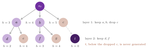
Figure 4.1; for the optimality, a goal at depth \(d\) may be
found before a cheaper one at a larger depth, since the layers are taken
by depth, whatever their cost. With \(B = \infty\) no node is dropped, and
line 8 keeps every node of next; by induction on \(d\), the layer \(d\)
then holds every state at the least depth \(d\) that is not a goal (a
state is first generated from the layer before its least depth, and it
may enter a later layer again only when its \(g\) falls), and the goals of
the least depth \(D\) are generated by the expansion of the layer \(D - 1\),
before which no goal is generated. \(\square\)
Also, the width \(B\) trades the quality of the path for the memory, and
the closed list of the library helps on graphs with many cycles, where
the same state would otherwise fill several layers. We remark that the
reopening changes the parent of a node after its successors have been
generated with the old \(g\): the cost returned is the \(g\) of the goal when
it was generated, whereas the path rebuilt from the parents at the end
may be another one, with more edges and a smaller cost (e.g., if \(a\),
reached first by an edge of cost 10 from \(s_0\), generates \(c\) and then
gets the parent \(b\) at the cost 2, the goal generated from \(c\) in the
next layer is returned with the path through \(b\) and the cost through
the edge of cost 10). Edelkamp and Schrödl
[10] describe the other variants (e.g., beams
on \(f\) instead of layers), and the beam-stack search of Zhou and Hansen
[117], which backtracks over the beams to
become complete, is not in the library. The test classic checks that the
beam of infinite width is optimal on 200 states of the 8-puzzle, whose
costs are uniform, that a beam of 2000 nodes returns a valid path on
instances of the 15-puzzle of Korf, and that a graph with no path is
reported unsolvable.
4.3 Depth-first branch-and-bound¶
Status — planned. The depth-first branch-and-bound of a
Domainis not in the library; the branch-and-bound searches of Chapter 13 offer it on a tree given by its branching, with the depth-first selection.
Depth-first branch-and-bound (DFBnB) searches the tree of the paths from \(s_0\) depth first, with the successors of a node taken by increasing \(h\), and prunes each node whose \(f\) is not less than the cost \(U\) of the best goal found so far (the incumbent); the memory is that of the current path and of the successors not yet tried along it.
Algorithm 4.2 (Depth-first branch-and-bound).
1  procedure DFBNB(u, g)
2     if g + h(u) ≥ U then return                           ▷ pruned
3     if u is a goal then U ← g;  record the path;  return
4     for each successor v of u, by increasing h(v) do
5        DFBNB(v, g + c(u, v))

   U ← ∞;  DFBNB(s₀, 0);  return the recorded path, if U < ∞
Proposition 4.3 (Optimality and memory of DFBnB). On a finite tree of depth \(D\), with \(h\) admissible, Algorithm 4.2 terminates, returns a path of cost \(C^*\) if a goal exists, and holds \(O(b D)\) nodes at a time.
Proof. The tree is finite and each node is visited at most once, hence the search terminates. Let \(P\) be an optimal path; the nodes \(u\) of \(P\) have \(g(u) + h(u) \le C^*\), by admissibility. While \(U > C^*\), no node of \(P\) is pruned at line 2, and the depth-first search, which visits each node that it does not prune, reaches the goal of \(P\) and sets \(U = C^*\); afterwards \(U\) never increases, and a goal recorded later would need \(g < U\). Hence the recorded path costs \(C^*\). The recursion has at most \(D + 1\) levels, each holding the at most \(b\) successors of its node sorted by \(h\). \(\square\)
Since the first goal is often found early and \(U\) only decreases, DFBnB is an "anytime" search, which can be stopped with the best path found so far; on a graph with cycles, however, the tree of its paths is infinite, and a depth bound (or an initial \(U\)) is needed for it to end. On a graph, moreover, DFBnB expands a state once per path that reaches it within the bound, the defect that the next section treats.
4.4 Iterative deepening¶
Depth-first iterative deepening (DFID, Korf [7]) runs a depth-first search bounded by the depth \(1, 2, 3, \ldots\) until a goal is found; with unit costs the first goal found is at the least depth, as with breadth-first search, while the memory is that of the current path. IDA\(^*\), also of Korf [7], replaces the depth by \(f = g + h\) and raises the bound, at each iteration, to the least \(f\) that exceeded the previous one; it is DFID when \(h = 0\) and the costs are 1 (Corollary 4.6).
The interface¶
IDAStar (IDAStar.h) searches a Domain with IDA\(^*\); its
declarations, without the bodies, are
struct IDAOptions : public SearchOptions , public DeepeningOptions {
 IDAOptions( void ) = default;
 IDAOptions( const SearchOptions & o );
 };

template< Domain D >
class IDAStar {
 public:
 explicit IDAStar( const D & domain , const IDAOptions & options = {} );
 [[nodiscard]] Solution< state_t< D > , cost_t< D > > solve( void ) const;
 [[nodiscard]] Solution< state_t< D > , cost_t< D > >
  solve( cost_t< D > bound ) const;
 };

template< Domain D >
[[nodiscard]] Solution< state_t< D > , cost_t< D > >
idastar( const D & domain , const IDAOptions & options = {} );

template< Domain D >
[[nodiscard]] Solution< state_t< D > , cost_t< D > >
cost_bounded_dfs( const D & domain , cost_t< D > bound ,
                  const SearchOptions & options = {} );
and idastar( domain , options ) is
IDAStar< D >( domain , options ).solve(). The Solution and the
SearchOptions are those of §1.5, and
IDAOptions adds to them the DeepeningOptions of IDA\(^*\)-CR, whose
growth (0 by default) and optimal choose the bounds of
§4.11; a SearchOptions converts to an IDAOptions with
the classical bounds. The second solve( bound ), which cost_bounded_dfs
calls, is one iteration with the given bound, the baseline of
§4.14. Of the options, node_limit bounds the expansions
(summed over the iterations), and the search stops with
Status::node_limit and an empty path when it reaches it;
expected_nodes is not used, since there is no CLOSED. With a weight
\(w > 1\) the bounds are on \(f' = g + w h\), and the path costs at most
\(w C^*\), since every node of an optimal path has \(f' \le w C^*\)
(Chapter 6); drop_duplicates does
nothing, there being no duplicate detection, and the constructor throws
std::invalid_argument if the options ask for an anytime search. The
status is solved with the cost and the path of the goal, or
unsolvable when an iteration cuts no node. In the counters of the
Solution, expanded counts every expansion, those repeated in later
iterations included, generated every successor that the domain passes
(those cut by the bound included, and, in a domain that is not an
OperatorDomain, the moves back to the parent too, which an
OperatorDomain does not pass at all), and stored the largest number
of states held on the path (Proposition 4.8); the field
bound of the Solution is, with \(w = 1\), the cost found, i.e., a
proof of optimality (with \(w > 1\), the cost over \(w\)), unless the bounds of IDA\(^*\)-CR end the search with a path
whose optimality they do not prove (Proposition 4.26). In
particular, one obtains DFID by giving IDAStar a Domain whose
heuristic returns 0.
IDA\(^*\)¶
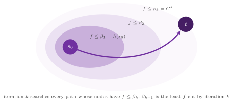
Each iteration of IDA\(^*\) is a depth-first search from \(s_0\) that cuts all the nodes with \(f > \beta\), the bound \(\beta\) being \(h(s_0)\) in the first iteration and, in each of the others, the least \(f\) that exceeded the bound of the previous one; the search ends when an iteration enters a goal, or with no goal reachable when no node was cut. Figure 4.2 shows the bounds as nested contours of \(f\).
The implementation makes the test of the bound when a successor is
generated, before entering it, and the goal test when a node is entered;
we say that a node is entered when the depth-first search is called on
it (and expanded when its successors are generated, which is the case
of every node entered that is not a goal), and cut when it is
generated with \(f > \beta\) and not entered. Also, the successors are
those of for_each_tree_child (Domain.h), passed one at a time,
without the move back to the parent on the path: by its operator in an
OperatorDomain, whose successor function skips the inverse of the
operator that generated the state, and otherwise by comparing the
successor with the state two places back on the path. In a
TreeOperatorDomain, for_each_tree_child calls
for_each_tree_successor( s , h , op , f ) instead, which may also skip
the successors of the pairs of moves (op, op\(_t\)) that the domain declares
redundant, because another sequence of moves that it keeps reaches the
same state at a cost not larger: two turns of the same face of Rubik's
cube, or of two opposite faces in the other order, and two moves of the
same disk of the Towers of Hanoi, as in Korf
[59]. The contract of the concept is that
every path is matched by a path with the same end, of a cost not larger,
whose moves are all kept; the searches with CLOSED do not use it, since
the path kept may go through a state closed with another operator, and
the test rubik checks the nodes of the tree of the cube at the depths 1
to 5, i.e., \(18\), \(243\), \(3240\), \(43254\) and \(577368\), against table 1 of
[59]. The following pseudocode is that of the
header IDAStar.h, i.e., the code of IDAStar::solve()
without the node limit, the counters and the bounds of IDA\(^*\)-CR.
Algorithm 4.3 (IDA\(^*\)).
 1  procedure IDA*(s₀)
 2     β ← h(s₀)
 3     loop
 4        β' ← ∞
 5        if DFS(s₀, 0, β) then return the path
 6        if β' = ∞ then return unsolvable
 7        β ← β'

 1  function DFS(u, g, β)                    ▷ g + h(u) ≤ β
 2     if u is a goal then return true
 3     for each successor v of u but the parent of u do
 4        g' ← g + c(u, v)
 5        if g' + h(v) > β then β' ← min(β', g' + h(v)); continue
 6        push v on the path
 7        if DFS(v, g', β) then return true
 8        pop v from the path
 9     return false
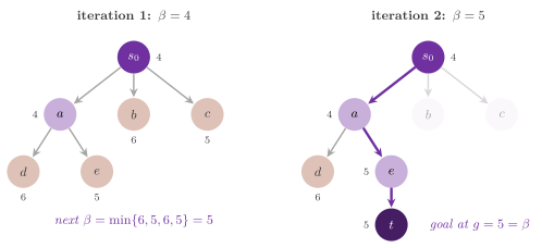
When a goal is entered, line 7 returns at once, the remaining successors of each node on the path being skipped, and the path is left from \(s_0\) to the goal. The node limit is tested when a node that is not a goal is entered, before its expansion; a goal is thus found even when the limit has just been reached. Figure 4.3 follows two iterations on a small tree. We now prove the properties of the algorithm (note that the proofs do not need a consistent heuristic), assuming an admissible heuristic, a finite branching factor and costs bounded below by some \(\varepsilon > 0\).
Lemma 4.4 (The bounds of IDA\(^*\)). If a goal is reachable, the bounds of the iterations increase strictly and none of them exceeds \(C^*\); furthermore, an iteration with \(\beta < C^*\) cuts at least one node with \(f \le C^*\).
Proof. The first bound is \(h(s_0) \le C^*\), by admissibility. Consider
an iteration with bound \(\beta < C^*\), and an optimal path \(P = (s_0 =
u_0, \ldots, u_k)\). The depth-first search enters \(s_0\) with \(g = 0 =
g^*(s_0)\). Suppose that it enters some \(u_j\), \(j < k\), with \(g =
g^*(u_j)\), along some path of that cost. Then it generates \(u_{j+1}\),
with \(g = g^*(u_{j+1})\), unless \(u_{j+1}\) is the parent \(w\) of \(u_j\) on
the path held. This is not the case: \(w\) has \(g^*(w) \le g^*(u_j) - c(w, u_j) <
g^*(u_j)\), whereas \(g^*(u_{j+1}) = g^*(u_j) + c(u_j, u_{j+1}) >
g^*(u_j)\), and hence \(u_{j+1} \ne w\) (with an OperatorDomain the
state skipped is \(w\) too, since the inverse of an operator leads back to
the state it came from, cf. §1.5). Thus
\(u_{j+1}\) is either cut or entered with \(g = g^*(u_{j+1})\). The search
cannot enter \(u_k\), since \(f(u_k) = C^* > \beta\), and an iteration that
enters some other goal first ends the search (which is then not of the
form considered here); also, an iteration that enters no goal visits
the whole tree of its paths within the bound, so that the generation
above does take place. Hence some \(u_{j+1}\) is cut, with \(f(u_{j+1}) =
g^*(u_{j+1}) + h(u_{j+1}) \le C^*\) by admissibility. The next bound is
the least \(f\) cut, which exceeds \(\beta\) (only nodes with \(f > \beta\)
are cut) and does not exceed \(f(u_{j+1}) \le C^*\). \(\square\)
In a TreeOperatorDomain the move from \(u_j\) to \(u_{j+1}\) may be one
that the domain skips after the move by which \(u_j\) was entered, and the
proof is then applied to an optimal path \(P\) whose moves are all kept,
which exists by the contract of the concept. The argument changes only
in that the iteration follows \(P\) itself, i.e., it enters each \(u_j\)
along the prefix of \(P\), since an iteration that enters no goal visits
every path of the tree of the kept moves whose nodes are within the
bound; the first node of \(P\) above the bound is then generated and cut.
The same holds for Theorem 4.5 and for the propositions
below.
Theorem 4.5 (Optimality of IDA\(^*\)). If \(h\) is admissible and a goal is reachable, Algorithm 4.3 returns a path of cost \(C^*\).
Proof. A goal \(t\) is entered only within the bound, i.e., with \(g(t) + h(t) \le \beta\); by admissibility \(h(t) = 0\), and by Lemma 4.4 \(\beta \le C^*\), so that \(g(t) \le C^*\), and hence \(g(t) = C^*\), since \(g(t)\) is the cost of a path. It remains to see that some iteration does enter a goal. By Lemma 4.4 the bounds increase strictly within the values of \(f\) not larger than \(C^*\) taken by the paths from \(s_0\), of which there are finitely many (a path of cost at most \(C^*\) has at most \(C^* / \varepsilon\) edges, and the branching is finite), and an iteration with \(\beta = C^*\) cannot cut a node of an optimal path, by the argument of the lemma, and therefore it enters the goal of one, if no goal was entered before. \(\square\)
Corollary 4.6 (DFID). With \(h = 0\) and unit costs, the bounds of Algorithm 4.3 are \(0, 1, 2, \ldots\), the iteration of bound \(\beta\) is the depth-first search to the depth \(\beta\), and the goal returned is at the least depth.
Proof. With \(h = 0\) and unit costs, \(f\) is the depth; a node cut by the iteration of bound \(\beta\) is at depth \(\beta + 1\), and hence each bound exceeds the previous one by 1 (an iteration that cuts no node ends the search). The least depth of a goal is \(C^*\), and the claim follows from Theorem 4.5. \(\square\)
Proposition 4.7 (Termination and number of iterations). (i) Each iteration ends, since it visits only paths of cost at most \(\beta\), which have at most \(\beta / \varepsilon\) edges. (ii) With integer costs and a reachable goal, IDA\(^*\) makes at most \(C^* - h(s_0) + 1\) iterations; on the sliding-tile puzzles with the Manhattan distance, at most \((C^* - h(s_0)) / 2 + 1\). (iii) If no goal is reachable, IDA\(^*\) reports it on a finite acyclic graph; on a graph with a reachable cycle that the parent pruning does not remove (e.g., a cycle of at least three states) it does not terminate, unless the node limit stops it.
Proof. (i) is the bound on the length of a path, together with the finite branching. (ii) By Lemma 4.4 the bounds are integers that increase strictly from \(h(s_0)\) to at most \(C^*\). On the puzzles a move changes \(g\) by 1 and the Manhattan distance by \(\pm 1\); hence, \(f\) changes by 0 or 2, and all the values of \(f\) have the parity of \(h(s_0)\), so that the bound increases by at least 2. (iii) On a finite acyclic graph the paths from \(s_0\) are finitely many; once the bound is at least the largest \(f\) on them, no node is cut, \(\beta' = \infty\), and line 6 reports the instance unsolvable. On a graph with a reachable cycle that the parent pruning does not remove, the paths that follow the cycle again and again are not pruned and have unbounded cost; for any \(\beta\), the first node with \(f > \beta\) on such a path is generated from an entered node and cut, and hence \(\beta' < \infty\) at every iteration. (A cycle \(u, v, u\) of two states is removed by the parent pruning, so that, e.g., on a finite undirected tree without a goal the search does terminate.) \(\square\)
Proposition 4.8 (The memory of IDA\(^*\)). At
any time, Algorithm 4.3 holds the path, of at most \(\lfloor \beta /
\varepsilon \rfloor + 1\) states, and one frame of the recursion per
state of the path; the successors are not stored, since they are passed
one at a time by the successor function of the domain (which may keep,
in each frame, the state of its own enumeration). If a goal is reachable,
the path never holds more than \(\lfloor C^* / \varepsilon \rfloor + 1\)
states; with unit costs and \(s_0\) not a goal, the counter stored of a
solved search is \(C^* + 1\).
Proof. Every state on the path is entered, with \(g \le \beta\), and the
path has at most \(\beta / \varepsilon\) edges; by Lemma 4.4
\(\beta \le C^*\). With unit costs a path of an iteration has at most \(C^*\)
edges, and the path returned has exactly \(C^*\) (Theorem
4.5); stored is the largest length of the path, measured
after each state pushed at line 6 of DFS, and hence it is \(C^* + 1\)
when at least one state is appended, i.e., when \(s_0\) is not a goal.
\(\square\)
The test idastar checks stored \(= C^* + 1\) on three instances of the
15-puzzle of Korf, the costs against the exact distances of 100 states
of the 8-puzzle and against A\(^*\) on small grids and on the map of
Romania, the report of an acyclic graph as unsolvable, and the stop at
1000 expansions. In fact, the cost of the repetitions is usually rather
small, as the next proposition shows, and the bound in (ii) of
Proposition 4.7 is the one of Exercise 4.5.
Proposition 4.9 (The overhead of the iterations). Let \(N_k\) be the expansions of the iteration \(k\), and let \(N_{k+1} \ge b' N_k\) for some \(b' > 1\) and all \(k\). Then the expansions of the \(K\) iterations sum to at most \(N_K \, b' / (b' - 1)\).
Proof. \(N_k \le N_K / b'^{K - k}\), and therefore \(\sum_{k=1}^{K} N_k \le N_K \sum_{j \ge 0} b'^{-j} = N_K \, b' / (b' - 1)\). \(\square\)
On a tree of uniform branching \(b\) and unit costs, DFID has \(b' = b\), and the overhead of the iterations is a factor of about \(b / (b - 1)\) over the last one (Korf [7]); IDA\(^*\) has a similar behavior when the number of nodes within the bound grows geometrically with it, as it is usually observed on the sliding-tile puzzles (an empirical fact, which the hypothesis of the proposition only models). In the worst case, however, each iteration adds a single node, the \(K\)-th iteration expands \(K\) nodes, and the total is \(K (K + 1) / 2\), i.e., quadratic in the expansions of A\(^*\) (e.g., with real costs that are all different).
Duplicate paths and parent pruning¶
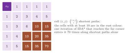
A depth-first search detects no duplicates: a state reached by several paths within the bound is expanded once per path in each iteration. On the sliding-tile puzzles the short cycles are rare, and IDA\(^*\) with a pattern database is the method of Korf and Felner [22] for the 24-puzzle (cf. Chapter 5); on the grids, on the contrary, a cell is reached by very many paths (Figure 4.4). Korf and Schultze give an order of magnitude for the 15-puzzle: a depth-first search to the average depth of an optimal solution, 53 moves, with the branching factor 2.13, would generate about \(2.5 \cdot 10^{17}\) nodes, against about \(10^{13}\) states [156].
The library prunes only the move back to the parent on the path, as described above. The pruning removes no optimal path, since an optimal path with positive costs has no cycle (cf. Proposition 2.16), and the proof of Lemma 4.4 shows that it never skips the next state of an optimal path.
Transposition tables¶
Status — planned.
IDAStarhas no transposition table.
A transposition table (§3.10) keeps, in a memory of fixed size, some of the states visited in the current iteration with the least \(g\) at which each was entered; a state reached again with a \(g\) not smaller than the one in the table is not entered, since everything below it was searched with a larger remaining budget (Reinefeld and Marsland [161] describe this and further uses of the table across the iterations). The pruning changes the least \(f\) that is cut, which may skip some values of the bound; the next proposition shows that the optimality survives.
Proposition 4.10 (Transposition tables keep IDA\(^*\) optimal). Let IDA\(^*\) skip, within an iteration, any state \(v\) reached with \(g \ge g_T(v)\), where \(g_T(v)\) is the least \(g\) with which \(v\) was entered earlier in the same iteration (and is kept in the table). Then, with \(h\) admissible, the bounds remain at most \(C^*\), and the path returned is optimal.
Proof. Let \(P = (s_0 = u_0, \ldots, u_k)\) be an optimal path and consider an iteration that enters no goal; let \(j\) be the largest index such that \(u_j\) is entered, at some time of the iteration, with \(g = g^*(u_j)\) (\(j \ge 0\), since \(s_0\) is entered with \(g = 0\)), and \(j < k\). At that entry \(u_{j+1}\) is generated with \(g^*(u_{j+1})\) (it is not the parent, as in Lemma 4.4). It is not entered with \(g^*(u_{j+1})\), by the choice of \(j\); nor is it skipped, since a skip needs an earlier entry with \(g_T(u_{j+1}) \le g^*(u_{j+1})\), i.e., with \(g^*(u_{j+1})\), again excluded by the choice of \(j\). Hence \(u_{j+1}\) is cut, with \(\beta < f(u_{j+1}) \le C^*\). Thus each iteration that ends without a goal has \(\beta < C^*\) and gives a next bound in \((\beta, C^*]\), which shows that the bounds increase strictly and stay at most \(C^*\); and an iteration with \(\beta = C^*\) cannot cut \(u_{j+1}\), so that it enters a goal. The rest of the proof of Theorem 4.5 applies unchanged. \(\square\)
We remark that the pruning may make IDA\(^*\) skip some intermediate values of the bound, never a value above \(C^*\); with a table of bounded size, entries are replaced, which only reduces the pruning.
Stochastic node caching¶
Status — planned.
Miura and Ishida [162] keep in a cache of bounded size a random subset of the states, each generated state being stored with a probability \(p\) if it is not cached yet; the cache is then filled mostly by the states that are generated often, i.e., by those reached along many paths (§3.10). The cached states are then used for duplicate detection, as in a transposition table, and the proof of Proposition 4.10 applies unchanged, since it holds for any content of the table.
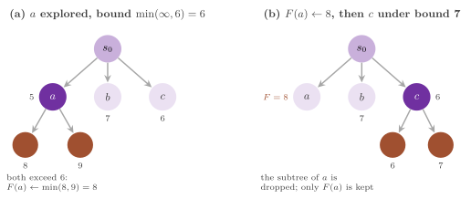
4.5 Recursive best-first search¶
Recursive best-first search (RBFS, Korf [116])
keeps, like IDA\(^*\), a single path, but with the siblings of its nodes,
and it expands the nodes in best-first order. Each node \(n\) carries a
stored value \(F(n) \ge f(n)\), initially \(f(n)\), the least \(f\) of the
frontier below it when it was last explored; the search below a node is
bounded by \(B\), the least stored value of the alternatives found higher
up, and when the subtree of a node exceeds its bound, the subtree is
dropped and its least \(f\) is backed up into \(F(n)\), so that the search
can return to it later without starting from scratch
(Figure 4.5). RBFS (RBFS.h) is the algorithm of
[116] with the pseudocode of the header.
Algorithm 4.4 (RBFS; \(c_1\) and \(c_2\) are the two successors of least \(F\), and \(F(c_2) = \infty\) when \(n\) has one successor).
 1  function RBFS(n, F(n), B)
 2     if f(n) > B then return f(n)
 3     if n is a goal then stop with the path to n
 4     if n has no successor then return ∞
 5     for each successor c of n do
 6        F(c) ← max(F(n), f(c)) if f(n) < F(n), else f(c)
 7     sort the successors by F
 8     while F(c₁) ≤ B and F(c₁) < ∞ do      ▷ c₁, c₂: the two best
 9        F(c₁) ← RBFS(c₁, F(c₁), min(B, F(c₂)));  sort again
10     return F(c₁)
11  RBFS(s₀, f(s₀), ∞)
Line 6 inherits the backed-up value of the parent: if \(F(n) > f(n)\), the
subtree of \(n\) was already explored up to \(F(n)\), and its successors are
given at least that value. In the code the successors of the node at the
depth \(d\) of the recursion are kept in a vector of that depth, reused
from one call to the next; they are those of for_each_child, without
the move back to the parent in an OperatorDomain (but with it
otherwise, since nothing compares a successor with the path), and a
successor of infinite \(h\) is not kept. After a call of line 9 the first
successor is moved back to its place by swaps with the following ones,
i.e., by one pass of insertion, the others being still sorted. The
declarations, quoted by hand, are
template< Domain D >
class RBFS {
 public:
 explicit RBFS( const D & domain , const SearchOptions & options = {} );
 [[nodiscard]] Solution< state_t< D > , cost_t< D > > solve( void );
 };

template< Domain D >
[[nodiscard]] Solution< state_t< D > , cost_t< D > >
rbfs( const D & domain , const SearchOptions & options = {} );
where the constructor throws std::invalid_argument for a weight other
than 1, node_limit bounds the expansions (the calls that reach line 5),
the stop at the limit returns Status::node_limit, and stored is the
largest number of successors held at a time on the path, i.e., the
memory of Proposition 4.11; bound is the cost of the path found.
Proposition 4.11 (The memory and the optimality of RBFS). (i) At any time, Algorithm 4.4 holds the nodes of the recursion and their successors, i.e., at most \(b\) nodes per level of the recursion, which is \(O(b D)\) for a recursion of depth \(D\). (ii) Let \(h\) be admissible, the branching finite, the costs at least some \(\varepsilon > 0\), and a goal reachable. Then every node that passes the test of line 2 has \(f \le C^*\), the recursion has a depth of at most \(C^* / \varepsilon + 1\), and Algorithm 4.4 terminates with a path of cost \(C^*\).
Proof. (i) A call holds its node and the list of its successors with their stored values (lines 5 to 10), and nothing else survives a return.
(ii) Fix an optimal path \(P = (s_0 = u_0, \ldots, u_k)\) without a cycle (one exists, the costs being positive). We say that a node \(x\) of the recursion is on \(P\) if the path of the recursion from \(s_0\) to \(x\) is a prefix of \(P\), in which case its \(g\) is \(g^*(x)\) and \(f(x) \le C^*\) by admissibility. We first show that \(F(x) \le C^*\) at any time for each successor \(x\) held that is on \(P\). When \(F(x)\) is set at line 6 it is \(f(x)\) or \(\max(F(n), f(x))\) for the parent \(n\) of \(x\), which is on \(P\) too, and the claim follows by induction on the depth (at the root, \(F(s_0) = f(s_0) \le C^*\)). When it is set at line 9, it is the value returned by RBFS\((x, \ldots)\), which is \(f(x) \le C^*\) at line 2, or not \(\infty\) at line 4, since the successor of \(x\) on \(P\) exists, is not the parent of \(x\) (\(P\) has no cycle) and has a finite \(h\) (\(h \le h^* < \infty\)), or the \(F\) of the best successor of \(x\) at line 10, which is at most the \(F\) of the successor of \(x\) on \(P\), at most \(C^*\) by induction on the number of the assignments.
Now consider any call RBFS\((n, F(n), B)\) while no goal has been found, and let \(x\) be the deepest node of the recursion path from \(s_0\) to \(n\) that is on \(P\). If \(x = n\), then \(f(n) \le C^*\). Otherwise the successor \(y\) of \(x\) on \(P\) is held, at the depth of \(x\), but it is not the successor \(c_1\) that the recursion follows; since \(c_1\) was chosen as the least by \(F\) and \(c_2\) as the second, \(F(c_2) \le F(y) \le C^*\), and every call below \(c_1\) receives a bound \(B \le F(c_2) \le C^*\), since the bound passed at line 9 only decreases with the depth. Hence a node that passes line 2 has \(f \le C^*\) in both cases. Its \(g\) is then at most \(C^*\), and its depth at most \(C^* / \varepsilon\), which bounds the recursion; the nodes at these depths are finitely many, and so are the values of \(f\) that can be returned at line 2, 4 or 10, i.e., the values of \(f\) of these nodes and of their successors, and \(\infty\).
A call of line 9 receives \(F(c_1) \le B' = \min(B, F(c_2))\) and, if it does not find a goal, returns a value larger than \(B'\) or \(\infty\) (by induction on the depth: line 2 returns \(f > B'\), line 4 returns \(\infty\), and line 10 returns an \(F\) that fails the test of line 8); hence each iteration of the loop of line 8 strictly raises \(F(c_1)\) within the finite set of the values above, and the loop ends. Since the recursion has a bounded depth, every call terminates. The root call cannot end without a goal: its loop ends only with \(F(c_1) = \infty\), whereas the successor of \(s_0\) on \(P\) has \(F \le C^*\). When a goal \(t\) is found, it passed line 2 with \(g(t) = f(t) \le C^*\) (\(h(t) = 0\) by admissibility), and \(g(t)\) is the cost of a path; thus \(g(t) = C^*\). \(\square\)
Korf [116] also proves that RBFS with a
consistent heuristic expands the new nodes in best-first order (his
theorems 4.2 and 4.3), which we do not reproduce; we checked only what
the proof above needs, i.e., the code of RBFS.h. Its weakness is
the same as that of IDA\(^*\), i.e., the regeneration of the dropped subtrees,
which may be frequent when the stored values of two siblings alternate as
the least, and the absence of duplicate detection, by which a state
reached by several paths is expanded once per path; on a grid with 4
moves the test classic runs it only on maps of \(8 \times 8\) cells, and
on the 15-puzzle on one instance of Korf, against the costs of A\(^*\) and
of the exact distances of 200 states of the 8-puzzle.
4.6 External search with delayed duplicate detection¶
IDA\(^*\) saves the memory of CLOSED by giving up the detection of the duplicates; an external search keeps it, but on the disk, where the time of an access is many orders of magnitude larger than in memory when it is random, and only somewhat larger when it is sequential. Hence the duplicates are not looked up when a node is generated, but detected later and in batches, by scanning files: this is the delayed duplicate detection (DDD) of §3.11, whose hash-based form is due to Korf [40].
Breadth-first search on the disk¶
The simplest case is the breadth-first search with unit costs. On an undirected graph the duplicates of a new layer are found in very few layers, as we now show; on a directed graph they may be in any earlier layer.
Proposition 4.12 (Duplicates of a breadth-first layer). On an undirected graph with unit costs, let \(L_i\) be the states at distance \(i\) from \(s_0\). A successor of a state of \(L_i\) is in \(L_{i-1}\), \(L_i\) or \(L_{i+1}\).
Proof. If \(v\) is adjacent to \(u \in L_i\), then \(\delta(v) \le \delta(u) + 1 = i + 1\) and, the graph being undirected, \(\delta(u) \le \delta(v) + 1\), i.e., \(\delta(v) \ge i - 1\), \(\delta\) denoting the distance from \(s_0\). \(\square\)
Hence, when the layer \(L_{i+1}\) is generated from \(L_i\), its duplicates are removed by comparing it with \(L_i\) and \(L_{i-1}\) only, and the older layers can be dropped (the frontier search of Korf et al., cf. [156]). The detection was first made by sorting the file of the new layer and merging it with the previous ones (sorting-based DDD); the hash-based DDD of Korf [40] avoids the sorting by two independent hash functions, a first one that splits the nodes into files (all the copies of a state are then in the same file), and a second one by which each file, loaded in a table in memory, drops its copies [156]. When the states have a perfect hash into a range that fits in memory at 2 bits per state, the two-bit breadth-first search of Korf [26] keeps instead, for each state, one of four values (not reached, in the current layer, in the next one, older) in an array of 2-bit entries; the library uses it to build the pattern databases (§5.5).
A\(^*\) with delayed duplicate detection: the interface¶
DDDAStar is the External A\(^*\) of Edelkamp, Jabbar and Schrödl
[39], with the hash-based DDD of Korf
[40] in place of the external sorts. It
requires a DiskDomain (DDDAStar.h:136), i.e., a Domain
with integer costs, since a bucket is a pair of values, and trivially copyable
states, since they are written to the files as their bytes. Its
declarations, without the bodies, are
template< DiskDomain D >
class DDDAStar {
 public:
 explicit DDDAStar( const D & domain , const SearchOptions & options = {} ,
                    DDDOptions ddd = {} );
 [[nodiscard]] Solution< state_t< D > , cost_t< D > > solve( void ) const;
 };

template< DiskDomain D >
[[nodiscard]] Solution< state_t< D > , cost_t< D > >
ddd_astar( const D & domain , const SearchOptions & options = {} ,
           const DDDOptions & ddd = {} );
where ddd_astar is DDDAStar< D >( domain , options , ddd ).solve(), and
the options of the disk are
struct DDDOptions {
 /// the files of a bucket, i.e., the parts by the hash of the state: the
 /// search holds in memory about the largest bucket over this number, with
 /// its copies, plus a buffer of buffer_bytes per file it writes and the
 /// buffer of the scans
 std::size_t partitions = 64;
 /// where the files go, in a directory of their own removed at the end;
 /// the temporary directory of the system if empty
 std::filesystem::path directory;
 /// the bytes of the buffer of each file being written, i.e., of each
 /// file of the buckets that the successors of a bucket go to
 std::size_t buffer_bytes = std::size_t( 1 ) << 16;
 };  // end( struct( DDDOptions ) )
i.e., the number \(P\) of files per bucket (partitions, 64 by default,
and 0 is refused with std::invalid_argument, as is a weight other than
1 in the SearchOptions), the directory of the
files (a directory of its own is made in it, or in the temporary
directory of the system when it is empty, and removed with its files at
the end, also when the search stops at the limit or throws), and the
bytes of the buffer of each file being written (buffer_bytes,
\(2^{16}\)). Of the SearchOptions, node_limit bounds the states
written to the closed files (the counter stored), checked after each
file, and expected_nodes is not used. In the counters, expanded
counts the states expanded, each once, generated the successors,
duplicates the copies dropped, and stored the states written to the
closed files, i.e., the distinct states closed.
The buckets and the files¶
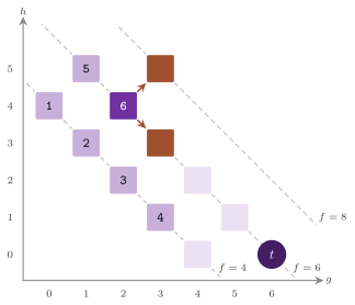
The nodes are kept in buckets \(B(g, h)\), one per pair of values, and
each bucket is split into \(P\) files by the hash of the state, the file
\(p\) holding the states \(v\) with \(\mathrm{hash}(v) \bmod P = p\); all the
copies of a state with the same \(g\) are thus in the same file, and all
those of the same state in the files of the same index \(p\), since \(h\) is
a function of the state. A record of a file is the state, the hash of
the state from which it was generated (its parent) and, in an
OperatorDomain, the operator that generated it. Each bucket has an
open part, the records appended to it and not yet examined, and a
closed part, the states of it that have been expanded. The buckets are
expanded by increasing \(f = g + h\) and, for equal \(f\), by increasing \(g\)
(i.e., the key of a bucket is the pair \((g + h, g)\), compared
lexicographically, cf. Figure 4.6).
Algorithm 4.5 (DDD-A\(^*\), the pseudocode of the header
DDDAStar.h:23-36).
 1  procedure DDD-A*(s₀)
 2     OPEN(0, h(s₀)) ← {s₀}
 3     while some OPEN(g, h) is not empty do
 4        (g, h) ← the bucket of least g + h, and then of least g
 5        for p ← 0 to P − 1 do
 6           T ← the states of the file p of OPEN(g, h), without copies
 7           for each closed bucket (g', h) with g' < g do
 8              T ← T ∖ the file p of CLOSED(g', h)
 9           the file p of CLOSED(g, h) ← T
10           if T has a goal then return the path to it, of cost g
11           for each u in T and each successor v of u do
12              append (v, hash(u)) to the file hash(v) mod P of
                 OPEN(g + c(u, v), h(v))
13     return unsolvable
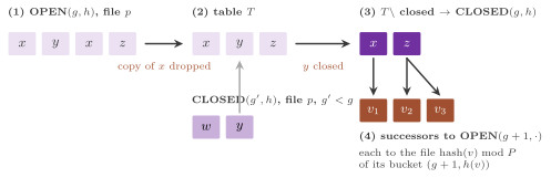
Lines 6 to 12 are the processing of one file, which the code does as
follows: the open file is loaded in a hash table of the memory, which
keeps the first record of each state; the closed files of the same \(h\)
are scanned, and the states found in them are removed from the table;
what is left is written as the closed file and expanded, each successor
being appended through a buffer per file of the buckets it goes to
(Figure 4.7). The expansion also checks the two hypotheses
on which the correctness rests, and throws std::logic_error on an edge
of a cost that is not positive or on a successor of a smaller \(f\) than
its parent, i.e., on a heuristic that is not consistent.
Algorithm 4.6 (The file \(p\) of the bucket \((g, h)\)).
 1  procedure FILE(g, h, p)
 2     T ← an empty hash table
 3     for each record (v, x, o) of the file p of OPEN(g, h) do
 4        if v ∈ T then count a duplicate else T[v] ← (x, o)
 5     delete the file p of OPEN(g, h)
 6     for each closed bucket (g', h) do                 ▷ all have g' < g
 7        for each record (v, ·, ·) of the file p of CLOSED(g', h) do
 8           if v ∈ T then remove v from T;  count a duplicate
 9     if T = ∅ then return
10     write the records of T as the file p of CLOSED(g, h)
11     if some state of T is a goal then
12        return TRACE(its record, g), of cost g             ▷ Algorithm 4.7
13     for each record (u, x, o) of T do
14        for each successor v of u but the inverse of o do
15           if c(u, v) ≤ 0 or g + c(u, v) + h(v) < g + h then
16              throw logic_error
17           append (v, hash(u), the operator of v) to the buffer of
18              the file hash(v) mod P of OPEN(g + c(u, v), h(v))
The buffers of the files written by a bucket are flushed when all its \(P\) files have been processed, and the buckets that they fill are then added to the open ones; the node limit is tested after line 18 of each file.
At the end the path is traced back from the goal through the hashes of the parents.
Algorithm 4.7 (The path to the goal of the record \(x\), closed with the cost \(g\)).
1  function TRACE(x, g)
2     π ← (the state of x)
3     while g ≠ 0 or the state of x ≠ s₀ do
4        p ← (the parent hash of x) mod P
5        y ← a record of the file p of some CLOSED(g', h'), g' < g,
6           whose state u has hash(u) = the parent hash of x and the
7           state of x as a successor of cost g − g'   ▷ else throw
8        x ← y;  g ← g';  prepend u to π
9     return π
Correctness¶
We now prove that the search is correct. Throughout, let \(h\) be
consistent (Definition 2.2) and 0 on the
goals (hence admissible, cf. §2.4), the
costs positive integers, and the inverse of the operator of a state, in
an OperatorDomain, lead back to the state that generated it.
Lemma 4.13 (The order of the buckets). A successor of a state of the bucket \((g, h)\) goes to a bucket of a larger key; hence no bucket receives a record after it has been expanded, and the buckets are expanded by increasing key.
Proof. A successor \(v\) of \(u\) has \(g(v) = g + c(u, v) > g\) and, by consistency, \(f(v) = g + c(u, v) + h(v) \ge g + h(u) = f(u)\); hence its key \((f(v), g(v))\) is larger than \((f(u), g)\). The search takes the open bucket of least key (line 4), and each bucket filled later has a larger key than the one being expanded. \(\square\)
Lemma 4.14 (Each state is closed once, at its optimal \(g\)). Every state \(v\) reachable from \(s_0\) whose bucket \((g^*(v), h(v))\) is expanded before the search stops is written to a closed file exactly once, in that bucket, and each other copy of it is dropped at line 4 or at line 8 of Algorithm 4.6; no state is written to two closed files.
Proof. Each copy of a state \(v\) carries the cost of a path to \(v\), hence \(g \ge g^*(v)\); all the copies of \(v\) have \(h(v)\) and lie in the files of index \(\mathrm{hash}(v) \bmod P\); and by Lemma 4.13 the buckets are expanded by increasing key \((g + h, g)\), so that among the buckets of \(h(v)\) the one of \(g^*(v)\) comes first. We prove by induction on the order of the expansions that, when a bucket \((g, h)\) is expanded, (a) every state \(v\) with \(g^*(v) = g\) and \(h(v) = h\) has a copy in it, and (b) a state of it is written to its closed file only if \(g = g^*(v)\) and it was not written before. For (a), \(s_0\) is put in \((0, h(s_0))\) by line 2 of Algorithm 4.5. Let \(v \ne s_0\), and \(w\) its predecessor on an optimal path, so that \(g^*(w) = g - c(w, v) < g\); the bucket \((g^*(w), h(w))\) has a smaller key (Lemma 4.13) and was expanded before, and by (a) and (b) for it \(w\) was written to its closed file there and expanded (the search did not stop, since it reached \((g, h)\)). The successor that line 14 of Algorithm 4.6 skips is the state \(u\) from which the record kept for \(w\) was generated, closed with some \(g_u\) such that \(g_u + c(u, w) = g^*(w)\); hence \(g^*(u) \le g_u < g^*(w) < g^*(v)\), and \(u \ne v\). Thus the expansion of \(w\) appended \(v\) with \(g^*(v)\) to \((g, h)\). For (b), a copy of \(v\) with \(g > g^*(v)\) is in a bucket that follows \((g^*(v), h)\), which by (a) held a copy of \(v\) and by (b) wrote \(v\) to its closed file of index \(\mathrm{hash}(v) \bmod P\) (no earlier closed file of \(h\) could hold \(v\), since it would have a smaller \(g\)); line 8 scans that file and removes \(v\). A state with \(g = g^*(v)\) is not in an earlier closed file, for the same reason, and line 4 keeps one record per state of a file. Hence each state whose bucket \((g^*(v), h(v))\) is expanded is written exactly once, there, and each other copy of it is dropped at line 4 or at line 8. \(\square\)
Theorem 4.15 (Correctness of DDD-A\(^*\)). If a goal is reachable, Algorithm 4.5 returns a path of cost \(C^*\) (when the node limit does not stop it first); otherwise, on a finite graph, it reports the instance unsolvable. In both cases it terminates, and each state is expanded at most once.
Proof. By Lemma 4.14 each state is written to a closed file at most once, and it is expanded only after that, i.e., at most once. Let a goal be reachable, and let \(t\) be an optimal one: \(t\) is closed in the bucket \((C^*, 0)\) if the search reaches it, and before it the open buckets are not exhausted, since by the induction of Lemma 4.14 the copies of the states of an optimal path reach their buckets. A goal closed earlier, in a bucket \((g, 0)\), has \(f = g\), and by Lemma 4.13 its bucket precedes \((C^*, 0)\) only if \(g \le C^*\); since \(g \ge C^*\) for a goal, the goal returned at line 10 has \(g = C^*\). By Proposition 4.17 the path returned costs \(g\). For the termination, the buckets with \(f \le C^*\) are finitely many (with integer costs, \(g \le C^*\) and \(h \le C^*\) in them). Each of them receives finitely many records: a record is a successor of a state closed in a bucket of smaller key, i.e., with \(g \le C^*\); these states have \(g^* \le C^*\), are finitely many (the branching being finite and the costs at least 1), and each is expanded once, with at most \(b\) successors. When no goal is reachable on a finite graph, the states are finitely many and each is expanded once, and hence the open buckets are eventually exhausted, and line 13 reports the instance unsolvable. \(\square\)
The counters follow from Lemma 4.14: each record of an open
file that is examined is either written to a closed file or dropped, and
hence one has \(\mathit{generated} + 1 = \mathit{stored} +
\mathit{duplicates}\) on a search that ends without a goal, the 1 being
the root, and \(\mathit{expanded} = \mathit{stored}\) (in a search that
stops at a goal the last file is closed but not expanded, and
\(\mathit{expanded} \le \mathit{stored}\)). The test ddd checks the
identity on a grid of \(50 \times 50\) cells split by a wall, where the
search closes the 1250 cells it can reach, the costs against the exact
distances of 50 states of the 8-puzzle with 1, 7 and 64 partitions,
against the optimal cost of an instance of the 15-puzzle of Korf, against
A\(^*\) on small grids, and on the map of Romania, the stop at the node
limit, the refusal of an inconsistent
heuristic and of no partition, and that no file is left on the disk.
Memory, files and the path¶
Proposition 4.16 (Memory and transfers of
DDD-A\(^*\)). At any time, the memory of Algorithm 4.5 holds (i) the hash
table of one file, sized for its records, copies included, and the
states left in it; (ii) a buffer of buffer_bytes bytes for each file
written by the current bucket, i.e., at most \(P\) for each distinct pair
\((g + c(u, v), h(v))\) of its successors; (iii) the buffer of the file
being read; and (iv) the sets of the open and of the closed buckets, one
entry per bucket. Each record of an open file is read once, and the
closed file \(p\) of a bucket \((g', h)\) is read once for each file \(p\) of a
later bucket of the same \(h\) that is not empty.
Proof. The table of a file and the states written from it (lines 2 to 10 of Algorithm 4.6) are released when the next file is processed; the writers of a bucket live until its \(P\) files are processed; the scans read through a buffer; and line 6 of Algorithm 4.6 runs over all the closed buckets of the same \(h\), all with a smaller \(g\) by Lemma 4.13. \(\square\)
Hence the memory is about that of the largest file, i.e., about \(1 / P\) of the largest bucket when the hash spreads the states evenly (an assumption on the hash of the domain), plus the buffers; with the defaults, a bucket whose successors go to \(k\) buckets holds \(64 k\) buffers of 64 KB, i.e., \(4 k\) MB. The files of all the closed buckets are kept to the end, since a duplicate may be in any of those with the same \(h\), and hence a closed file is read once for each later bucket of its \(h\). Of course, on the undirected graphs with unit costs one could drop the older layers, as in Proposition 4.12, which the library does not do, since it assumes no locality of the domain. Note also that the order by increasing \(g\) within a layer of \(f\), which Lemma 4.13 requires, is the opposite of the tie-breaking of A\(^*\) (§2.8): the search expands every state of the last layer \(f = C^*\) that it generates before the bucket of the goal, and it may expand many more nodes than A\(^*\) when that layer is large.
Proposition 4.17 (The path). Under the hypotheses of Lemma 4.14, Algorithm 4.7 never throws, terminates, and returns a path from \(s_0\) to the goal of cost \(g\); each step reads at most all the closed files of one partition.
Proof. The record \(x\) kept for a state \(v\) closed with \(g\) was generated from a state \(w\) that was closed in a bucket \((g_w, h(w))\) with \(g_w + c(w, v) = g\), and hence \(g_w < g\), in the file \(\mathrm{hash}(w) \bmod P\), which is kept to the end; thus a record \(y\) as at lines 5 to 7 exists (it may be another state with the same hash, which is still a predecessor of \(v\) at the cost \(g - g'\)). The state \(u\) of \(y\) was closed with \(g'\), and the invariant of the loop is that \(\pi\) is a path from the state of \(x\) to the goal of cost \(g_0 - g\), \(g_0\) being the cost of the goal. Since \(g\) decreases strictly and is a nonnegative integer, the loop ends; it ends only with \(g = 0\) and the state \(s_0\), and then \(\pi\) has the cost \(g_0\). The only state closed with \(g = 0\) is \(s_0\), since the costs are positive; hence the loop cannot reach \(g = 0\) elsewhere. \(\square\)
4.7 Symbolic search¶
Status — planned. The library has no symbolic search.
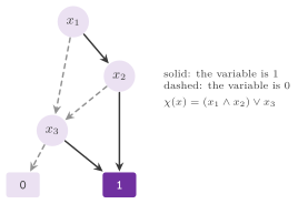
A symbolic search represents whole sets of states by their characteristic functions. With the states coded by \(n\) Boolean variables \(x = (x_1, \ldots, x_n)\), a set \(S\) is the function \(\chi_S(x)\), true exactly on the codes of the states of \(S\), and the moves are a transition relation \(\mathit{Trans}(x, x')\), true when the state \(x'\) is a successor of \(x\). The image of a set is $\(\mathit{Img}(S)(x') = \exists x \, \big( \chi_S(x) \wedge \mathit{Trans}(x, x') \big),\)$ renamed from \(x'\) to \(x\); it is the set of the successors of the states of \(S\), computed in one operation on the functions. The functions are represented by reduced ordered binary decision diagrams (BDDs), i.e., directed acyclic graphs in which each node tests a variable, in a fixed order, with two successors for its values, and the leaves are 0 and 1 (Figure 4.8). For a fixed order of the variables the reduced ordered BDD of a function is unique (Bryant [163]); hence, the equality of two sets is a comparison of two pointers when the BDDs share their nodes, and the operations \(\wedge\), \(\vee\), \(\neg\) take a time polynomial in the sizes of the operands [163]; the size of a BDD, however, depends heavily on the order, and may be exponential in \(n\).
Algorithm 4.8 (Symbolic breadth-first search).
1  procedure SYMBOLIC-BFS(s₀)
2     Reach ← {s₀};  Frontier ← {s₀};  d ← 0         ▷ as BDDs
3     loop
4        if Frontier ∩ Goals ≠ ∅ then return d
5        Frontier ← Img(Frontier) ∖ Reach
6        if Frontier = ∅ then return unsolvable
7        Reach ← Reach ∪ Frontier;  d ← d + 1
Proposition 4.18 (Symbolic breadth-first search). At line 4 of the iteration \(d\), Frontier is the set of the states at distance \(d\) from \(s_0\) (with unit costs) and Reach the set of those at distance at most \(d\); hence Algorithm 4.8 returns the least distance of a goal, and on a finite space it terminates.
Proof. By induction on \(d\). For \(d = 0\) both sets are \(\{s_0\}\). If the claim holds for \(d\), the successors of the states at distance \(d\) that are not at distance at most \(d\) are those at distance \(d + 1\), which is line 5, and line 7 adds them to Reach. The first \(d\) at which the frontier meets the goals is the least distance of a goal; on a finite space Reach grows strictly until the frontier is empty. \(\square\)
One can rebuild the path backwards, by intersecting the preimage of the goal reached with the frontiers kept for the purpose. Symbolic A\(^*\) keeps instead one BDD per bucket of \((g, h)\), or of \((f, h)\), and expands the buckets in the order of A\(^*\), as DDD-A\(^*\) does with its files (cf. Edelkamp and Schrödl [10]).
4.8 Novelty and width-based search¶
Let a state be described by the values of \(m\) variables, and call an atom a pair (variable, value). The novelty of a newly generated state \(s\) is the least \(i\) such that some set of \(i\) atoms true in \(s\) is true in no state generated before \(s\). The search IW\((i)\) of Lipovetzky and Geffner [104] is a breadth-first search that prunes each generated state of novelty larger than \(i\); its memory is that of the sets of at most \(i\) atoms seen so far, and the iterated width runs IW\((1)\), IW\((2)\), ... until a goal is found.
Algorithm 4.9 (IW\((i)\)).
1  procedure IW(s₀, i)
2     Seen ← the sets of at most i atoms true in s₀;  Q ← (s₀)
3     while Q is not empty do
4        u ← the first node of Q, removed
5        if u is a goal then return the path to u
6        for each successor v of u do
7           if some set of at most i atoms of v is not in Seen then
8              add those sets to Seen;  append v to Q
9     return failure
Proposition 4.19 (The size of IW\((i)\)). With \(m\) variables of at most \(D\) values each, IW\((i)\) appends at most \(\sum_{j=1}^{i} \binom{m}{j} D^j = O\big((m D)^i\big)\) states to Q. Furthermore, the iterated width finds a goal, if one is reachable, at the latest with \(i = m\).
Proof. A state appended at line 8 adds at least one set of at most \(i\) atoms to Seen, which never loses one; the sets of \(j\) atoms over distinct variables are at most \(\binom{m}{j} D^j\). With \(i = m\), a state not generated before has the set of all its \(m\) atoms unseen, since the \(m\) atoms determine the state, while a state generated before has all its sets in Seen; hence IW\((m)\) is a breadth-first search with duplicate detection, which is complete on a finite space. \(\square\)
The library implements IW\((i)\) (IteratedWidth), the serialized width
search SIW (SerializedWidth) and the best-first width search BFWS
(BestFirstWidth) in WidthSearch.h, over the features of a
FeatureDomain rather than the atoms of variables, with the novelty
kept by a NoveltyTable; they are described in full, with their options
and their tests, in §2.15, and here we only
place them among the searches that bound what they keep. We remark that
IW\((i)\) for small \(i\) is neither complete nor optimal;
its interest is that many classical planning problems with single atomic
goals have a small width, and IW\((1)\) or IW\((2)\) solves them in time
polynomial in \(m\) [104] (cf.
Chapter 16).
4.9 Partial expansion¶
A\(^*\) puts in OPEN every successor of a node that it expands, and on a domain with a large branching factor most of them have \(f > C^*\), i.e., they are surplus nodes, which are stored and never expanded. Partial Expansion A\(^*\) (PEA\(^*\), Yoshizumi, Miura and Ishida [42]) stores only the successors whose \(f\) is within a cutoff of the value of their parent, and keeps the parent in OPEN with the least \(f\) of the others; Enhanced Partial Expansion A\(^*\) (EPEA\(^*\), Felner et al. [113] and Goldenberg et al. [114]) does not even generate the others, since the domain tells which successors have the value sought.
Both keep with a node \(n\) a stored value \(F(n) \ge f(n)\), \(f(n)\) when \(n\) gets a new \(g\), by which OPEN is ordered, the ties going to the larger \(g\). When \(n\) is selected, only its successors \(c\) with \(f(c) \le F(n) + C\) (PEA\(^*\), \(C \ge 0\) being the cutoff) or with \(f(c) = F(n)\) (EPEA\(^*\)) are put in OPEN, and \(n\) goes back to OPEN with \(F(n)\) the least \(f\) of the others, if any, or is closed otherwise. We write \(\Delta f(c) = f(c) - f(n) = c(n, c) + h(c) - h(n)\) for a successor \(c\) of \(n\); with a consistent heuristic \(\Delta f \ge 0\) on every edge.
Algorithm 4.10 (PEA\(^*\) and EPEA\(^*\), the pseudocode of the header
PartialExpansion.h).
 1  procedure PEA*(s₀)                     ▷ EPEA* at the lines marked E
 2     F(s₀) ← f(s₀);  push s₀ in OPEN, by F and then by larger g
 3     while OPEN ≠ ∅ do
 4        n ← the first node of OPEN, removed;  if n is a goal then
             return the path to n
 5        generate the successors c of n         ▷ E: those with
             f(c) − f(n) = F(n) − f(n) only, by the operator selection
             function, which also gives the least larger Δf
 6        for each c with f(c) ≤ F(n) + C do
 7           if c is new or reached through a cheaper path then
                F(c) ← f(c);  push c in OPEN
 8        F' ← the least f(c) > F(n) + C of the others that are new or
             reached through a cheaper path (E: f(n) plus the least
             larger Δf of all the others), ∞ if none
 9        if F' < ∞ then F(n) ← F';  push n in OPEN again
10        else close n
The operator selection function of EPEA\(^*\) is the method
for_each_successor_delta( s , h_s , op , delta , f ) of a
PartialExpansionDomain (Domain.h), an OperatorDomain that
calls f( t , c , h_t , op_t ) for the successors \(t\) of \(s\) whose \(\Delta f\)
is delta (with real costs, up to a slack such as that of
cost_slack()), without the one that the inverse of op leads to, and
returns the least \(\Delta f\) above delta of the others, or
infinite_cost() if there is none. On the sliding-tile puzzles a move
costs 1 and changes the Manhattan distance by \(\pm 1\), so that \(\Delta f
\in \{0, 2\}\) is read from the table of the distances without building
the successor; on the grids it depends on the cost of the cell entered
and on the octile distance (Chapter 14).
Line 8 of PEA\(^*\) leaves out of \(F'\) the successors already stored with
a \(g\) not larger than \(g(n) + c(n, c)\) (PartialOptions::skip_known, true
by default), which line 7 would reject at every later selection of \(n\)
with the same \(g(n)\); the comparisons of line 6 allow, with real costs,
the slack \(\tau \max\{1, |F(n)|\}\) of cost_slack(), \(\tau\) being
PartialOptions::tolerance (\(10^{-9}\) by default), so that two values of
\(f\) that are equal but for the rounding of sums of the same costs in
another order do not cost a selection each. EPEA\(^*\) keeps with a node,
with real costs, the \(\Delta f\) of its next selection, since \(F(n) -
f(n)\) need not be exact; with integer costs it computes it as \(F(n) -
f(n)\). The options of PEA\(^*\) are
struct PartialOptions : public SearchOptions {

 /// the cutoff C of PEA*: the successors with \f$ f \leq F( n ) + C \f$
 /// enter OPEN at a selection of n
 double cutoff = 0;

 /// leave out of the next \f$ F( n ) \f$ the successors already stored
 /// with a g not larger than the one through n
 bool skip_known = true;

 /// the relative tolerance of the comparisons of f with
 /// \f$ F( n ) + C \f$, for real costs [see cost_slack()]
 double tolerance = real_cost_tolerance;

 };  // end( struct( PartialOptions ) )
and the declarations, quoted by hand, are
template< Domain D >
class PEAStar : public PartialExpansionBase< D , PEAStar< D > > {
 public:
 explicit PEAStar( const D & domain , const PartialOptions & options = {} );
 [[nodiscard]] Solution< state_t< D > , cost_t< D > > solve( void ) const;
 };

template< PartialExpansionDomain D >
class EPEAStar : public PartialExpansionBase< D , EPEAStar< D > ,
                                              PartialExtra< cost_t< D > > > {
 public:
 explicit EPEAStar( const D & domain , const SearchOptions & options = {} );
 [[nodiscard]] Solution< state_t< D > , cost_t< D > > solve( void ) const;
 };

template< Domain D >
[[nodiscard]] Solution< state_t< D > , cost_t< D > >
pea_star( const D & domain , const PartialOptions & options = {} );

template< PartialExpansionDomain D >
[[nodiscard]] Solution< state_t< D > , cost_t< D > >
epea_star( const D & domain , const SearchOptions & options = {} );
The two searches share the class template PartialExpansionBase< D ,
Derived , Extra >, which holds the nodes (with \(F\) and the value of type
Extra that the derived class keeps, value-initialized when a node gets
a new \(g\)), CLOSED, OPEN (a \(d\)-ary heap of entries \((F, g, n)\), an entry
being stale when its node is closed or has another \(g\) or another \(F\))
and the loop of lines 3 to 10, and calls the method expand( n , run )
of Derived for lines 5 to 8, i.e., the static polymorphism of the
curiously recurring template. Extra is PartialNoExtra, an empty
struct, for PEA\(^*\) and for EPEA\(^*\) with integer costs, and
PartialDelta< Cost >, which holds the \(\Delta f\) of the next selection,
for EPEA\(^*\) with real costs (the alias PartialExtra< Cost > chooses
between them). Both constructors throw std::invalid_argument for a
weight other than 1; node_limit bounds the stored nodes, expanded
counts the selections and reexpanded those of a node selected before,
generated counts every successor generated by PEA\(^*\) but only those
passed by the operator selection function for EPEA\(^*\), and duplicates
counts, for PEA\(^*\), also the successors left out of \(F'\) as known.
We now prove that the skip of the known successors loses nothing, and then the optimality of both searches; the argument adapts the invariant of OPEN of A\(^*\) (Lemma 2.7) to the stored values.
Lemma 4.20 (The skip of the known successors).
Let \(v\) be a successor of \(n\) left out of \(F'\) at a selection of \(n\) by
skip_known. Then every later generation of \(v\) from \(n\) with the same
\(g(n)\) is rejected as a duplicate at line 7, and every selection that the
skip removes is one that would put no node in OPEN through \(v\).
Proof. The stored \(g(v)\) never increases, and \(v\) is put in OPEN through \(n\) only if \(g(n) + c(n, v) < g(v)\); since \(v\) was left out with \(g(v) \le g(n) + c(n, v)\), as long as \(g(n)\) does not change \(v\) is rejected at every later selection of \(n\). A smaller \(g(n)\), on the other hand, puts \(n\) back in OPEN with \(F(n) = f(n)\), and then all its successors are examined again with the new \(g(n)\). \(\square\)
Theorem 4.21 (Optimality of PEA\(^*\) and
EPEA\(^*\)). Let \(h\) be admissible, and for EPEA\(^*\) also consistent (it
suffices that \(\Delta f \ge 0\) on every edge). Then, as long as the
search runs, OPEN holds a non-stale entry with \(F \le C^*\) (up to the
slack of the real costs), and the first goal selected has \(g = C^*\);
this holds for any cutoff \(C \ge 0\), with or without skip_known.
Proof. Let \(P\) be an optimal path to a goal \(t\). If all its nodes are
stored with their optimal \(g\), then \(t\) is in OPEN with \(F(t) = f(t) =
C^*\), since a goal is never expanded (its selection ends the search).
Otherwise, let \(u\) be the first node of \(P\) whose successor \(v\) on \(P\) is
not stored with \(g(v) = g^*(v)\); then \(u\) is stored with \(g(u) =
g^*(u)\), being \(s_0\) or the successor of a node of \(P\) before it. At no
selection of \(u\) with this \(g\) has \(v\) been put in OPEN through \(u\),
which would give \(g(v) \le g^*(u) + c(u, v) = g^*(v)\), nor left out of
\(F'\) by skip_known, which needs a stored \(g(v) \le g^*(v)\), nor
rejected at line 7, for the same reason.
For PEA\(^*\), at each such selection \(v\) was therefore one of the others of line 8, with \(f(v) > F(u) + C\), and \(F'\) was at most \(f(v)\); hence \(u\) is not closed, and \(F(u)\) is either \(f(u) \le C^*\) (before its first selection with this \(g\)) or at most \(f(v) = g^*(v) + h(v) \le C^*\). For EPEA\(^*\), let \(\delta\) be the \(\Delta f\) of a selection of \(u\), \(0\) at the first one. If \(\Delta f(v) = \delta\), the operator selection function would pass \(v\), which then would be stored with \(g^*(v)\); thus \(\Delta f(v) \ne \delta\). Since \(\delta = 0 \le \Delta f(v)\) at the first selection, and each later \(\delta\) is the least \(\Delta f\) above the one before among the successors not passed, \(v\) among them, by induction \(\delta < \Delta f(v)\) at every selection, and the next one is at most \(\Delta f(v)\); hence \(u\) is not closed, and \(F(u) = f(u) + \delta \le f(u) + \Delta f(v) = f(v) \le C^*\).
In both cases the entry pushed with the current \(F(u)\) and \(g(u)\) is not stale, and OPEN holds an entry with \(F \le C^*\). The entry selected has the least \(F\); when it is a goal \(t'\), its \(F\) is \(f(t') = g(t')\), since a goal is pushed only by line 7 and never selected twice, and therefore \(g(t') \le C^*\); finally \(g(t') \ge C^*\), being the cost of a path. With real costs the comparisons of line 6 and the grouping of \(\Delta f\) by the domain only widen the set of the successors put in OPEN by the slack, which the argument absorbs as it absorbs \(C\). \(\square\)
The consistency matters to EPEA\(^*\) only: with a \(\Delta f < 0\) on an edge, the first selection asks for \(\Delta f = 0\) and the next ones for larger values, so that the successor of that edge is never generated through it, which the pseudocode of the header does not exclude and the library does not check. PEA\(^*\), on the contrary, puts in OPEN every successor of \(f \le F(n) + C\), including those of a smaller \(f\).
Proposition 4.22 (What partial expansion stores and generates). Under the hypotheses of Theorem 4.21, every node put in OPEN by PEA\(^*\) before the end has \(f \le C^* + C\) (up to the slack), and every node put in OPEN by EPEA\(^*\) has \(f \le C^*\); hence the surplus nodes, of \(f > C^* + C\) and of \(f > C^*\) respectively, are never stored. A selection of EPEA\(^*\) generates only nodes that it puts in OPEN or finds to be duplicates, and each of them at most once per selection.
Proof. By Theorem 4.21 each entry selected before the end has \(F \le C^*\), and line 6 puts in OPEN only successors with \(f \le F + C\); EPEA\(^*\) puts in OPEN only successors with \(f = F\). The last claim is the definition of the operator selection function, which passes each successor whose \(\Delta f\) is \(\delta\) once, and nothing else. \(\square\)
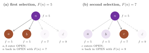
The price is time: PEA\(^*\) generates all the successors of a node at
each of its selections, and a node with \(m\) distinct values of \(f\) among
its successors may be selected \(m\) times; EPEA\(^*\) saves the
generations, but it cannot leave out the known successors without
generating them, so that it makes the selections of PEA\(^*\) without the
skip while generating fewer nodes. We remark that the lemma does not
bound the number of the selections of PEA\(^*\) with the skip by that of
PEA\(^*\) without it, since the order of the ties of OPEN may change; the
test classic checks that it is not larger on the grids of \(60 \times 60\)
cells of three random maps with 4 and 8 moves, that neither is larger
than the selections of the code before the skip (466, 750 and 574 with 4
moves, 752, 2167 and 1495 with 8), and that EPEA\(^*\) generates fewer
nodes than PEA\(^*\); on instances of the 15-puzzle of Korf, EPEA\(^*\)
generates and stores fewer nodes than A\(^*\), and PEA\(^*\) stores fewer.
Figure 4.9 follows the selections of a node.
4.10 Fringe search¶
IDA\(^*\) starts each iteration from the root and regenerates every node of the iterations before; fringe search, of Björnsson, Enzenberger, Holte and Schaeffer [115], keeps instead the frontier of IDA\(^*\), the fringe, in a list \(L\), so that an iteration starts from the nodes where the one before stopped, and the \(g\) of every state seen in a cache \(C\), so that a state is not expanded again through a path that is not cheaper. Its memory is that of A\(^*\), while its time per node is smaller, since the list costs \(O(1)\) per operation instead of the \(O(\log n)\) of a heap, at the price of visiting the nodes of the fringe above the threshold at each iteration.
Algorithm 4.11 (Fringe search, the pseudocode of the header
FringeSearch.h).
 1  procedure FRINGE(s₀)
 2     L ← ⟨s₀⟩;  C[s₀] ← (0, nil);  θ ← h(s₀)
 3     while L ≠ ⟨⟩ do
 4        θ' ← ∞
 5        for each node n of L, from the first to the last do
 6           if g(n) + h(n) > θ then θ' ← min(θ', g(n) + h(n));  continue
 7           if n is a goal then return the path to n
 8           for each successor c of n do
 9              g' ← g(n) + c(n, c)
10              if c ∈ C and g' ≥ g(c) then continue
11              remove c from L if it is there;  C[c] ← (g', n)
12              insert c in L just after n
13           remove n from L
14        θ ← θ'
The list is doubly linked through the nodes of the cache, with a
sentinel, and a flag tells whether a node is in it; the successors are
those of for_each_child, inserted after \(n\) in the order of their
generation, so that they are visited right after their parent, which is
the depth-first order of IDA\(^*\). The declarations, quoted by hand, are
template< Domain D >
class FringeSearch {
 public:
 explicit FringeSearch( const D & domain ,
                        const SearchOptions & options = {} );
 [[nodiscard]] Solution< state_t< D > , cost_t< D > > solve( void );
 [[nodiscard]] std::size_t iterations( void ) const noexcept;
 };

template< Domain D >
[[nodiscard]] Solution< state_t< D > , cost_t< D > >
fringe_search( const D & domain , const SearchOptions & options = {} );
where the constructor throws std::invalid_argument for a weight other
than 1, iterations() gives the passes of the last search, node_limit
bounds the nodes of the cache, tested after each expansion, expanded
counts the expansions (line 8), reexpanded those of a state expanded
before, and stored the states of the cache.
Theorem 4.23 (Optimality and termination of
fringe search). Let \(h\) be admissible and finite on the states that the
search meets. (i) At the start of each pass the
threshold satisfies \(\theta \le C^*\), the thresholds increase strictly,
and the first goal found has \(g = C^*\). (ii) On a finite graph Algorithm
4.11 terminates, and it returns unsolvable if no goal is reachable.
Proof. We first show an invariant: a state of \(C\) that has not been expanded with its current \(g\) is in \(L\). Indeed, a state gets a new \(g\) only at line 11, after which line 12 inserts it in \(L\), and it leaves \(L\) only at line 11, to be inserted again, or at line 13, after its expansion. Let \(P\) be an optimal path whose goal has not been returned, and \(u\) the first node of \(P\) that has not been expanded with \(g = g^*(u)\). Then \(u = s_0\), which is in \(L\) with \(g = 0\), or the predecessor \(p\) of \(u\) on \(P\) was expanded with \(g^*(p)\), which gave \(u\) the value \(g^*(u)\) at line 11 or found it there already (line 10); since \(g\) cannot fall below \(g^*\), it has not changed since, and by the invariant \(u\) is in \(L\) with \(g(u) = g^*(u)\), i.e., \(f(u) \le C^*\).
(i) Consider a pass that returns no goal. Every node in \(L\) at its end was visited by the pass, since a node is always inserted just after the node being expanded, i.e., ahead of the scan; and at its last visit it was skipped at line 6 with its current \(g\), since a change of \(g\) after the visit would have moved it ahead of the scan again, and an expansion would have removed it. Hence \(u\) was skipped with \(f(u) > \theta\), and \(\theta' \le f(u) \le C^*\), while \(\theta' > \theta\) since only the nodes above \(\theta\) contribute to it. The first threshold is \(h(s_0) \le C^*\), and by induction \(\theta \le C^*\) at each pass. A goal \(t\) is returned only within the threshold, with \(h(t) = 0\), and thus \(g(t) \le \theta \le C^*\), while \(g(t) \ge C^*\), being the cost of a path. (ii) On a finite graph the values of \(g\) of a state are finitely many and strictly decreasing (the argument of Theorem 2.11), each insertion in \(L\) is paid by one of them, and a pass ends; the thresholds are values of \(f\) of these pairs, finitely many, and increase strictly. If no goal is reachable, every state of \(C\) is eventually expanded with its last \(g\), and \(L\) empties. \(\square\)
On an infinite graph with finite branching and costs at least
\(\varepsilon > 0\), the argument of (ii) of
Theorem 2.11 applies in the same way, since
each node expanded has \(g \le \theta \le C^*\). We remark that the cost
returned is the \(g\) of the goal, and that the path is that of its
parents: with an admissible \(h\) both are \(C^*\), since the path rebuilt
costs at most \(g(t)\) and at least \(C^*\). The test classic checks the
costs on 200 states of the 8-puzzle, on instances of the 15-puzzle of
Korf and on grids of \(50 \times 50\) cells with 8 moves, the node limit,
and a graph with no path. The finiteness of \(h\) is needed by the code, and
not only by the proof: a dead end whose \(h\) is infinite_cost() makes
\(g + h\) overflow with integer costs
(FringeSearch.h:155), whereas BeamSearch and RBFS
drop such a successor when it is generated.
4.11 The bounds of iterative deepening¶
An iteration of IDA\(^*\) of bound \(\beta_k\) prunes the nodes of \(f > \beta_k\), and the classical next bound is the least of their \(f\), \(\ell_k\), so that each iteration adds at least one value of \(f\). When the values of \(f\) are many and close, e.g., with costs that are not integers, or on the grids, whose number of nodes grows slowly with the bound, the iterations are as many as the values of \(f\) below \(C^*\), and the search expands the nodes of the first ones again at each of them, i.e., quadratically many times in the worst case of Proposition 4.9. IDA\(^*\)-CR, of Sarkar, Chakrabarti, Ghose and De Sarkar [132], chooses instead a bound beyond which enough pruned nodes lie, so that the iterations grow geometrically, and pays for it with an iteration whose bound may exceed \(C^*\).
The options are those of DeepeningOptions (Deepening.h),
which IDAOptions inherits and which the iterative-deepening searches of the
parallel chapters share:
struct DeepeningOptions {

 /// the growth \f$ r \f$ of IDA*-CR: if larger than 1, the next bound is
 /// the one of CutoffHistogram, otherwise the least f pruned
 double growth = 0;

 /// true to complete the iteration of the first goal as a branch-and-bound
 /// when its bound is above the least f pruned by the iteration before, so
 /// that the path is optimal; false to stop at the first goal, whose cost
 /// is then within \f$ \beta_{k+1} - \ell_k \f$ of the optimum
 bool optimal = true;

 };  // end( struct( DeepeningOptions ) )
With the growth $r = $ growth \(> 1\), the next bound is chosen by a
CutoffHistogram< Cost >, in which each iteration records the \(f\) of
the nodes that it prunes; its interface, quoted by hand without the
bodies, is
template< class Cost >
class CutoffHistogram {
 public:
 void reset( Cost b , bool buckets ) noexcept;
 void restart( void ) noexcept;
 void add( Cost f ) noexcept;
 void merge( const CutoffHistogram & o ) noexcept;
 [[nodiscard]] Cost low( void ) const noexcept;
 Cost next( double growth , std::uint64_t expanded );
 };
where reset( b , buckets ) empties it for the iteration of bound \(b\)
(counting the \(f\) in buckets only if buckets), restart() forgets the
last step, add( f ) records a node of \(f > b\), merge( o ) adds the
nodes of another histogram of the same iteration (that of another
worker, in a parallel search), low() is \(\ell_k\), and next( r , E_k )
is the next bound for an iteration of \(E_k\) expansions. The buckets are
those of the binary exponent of the excess \(f - \beta_k\), the excesses in
\([2^{x-1}, 2^x)\) in the bucket \(x\), so that the histogram has a fixed
size whatever the costs (2100 buckets, one per exponent of a
double), and its buckets are fine near the bound and coarse far from
it. The rule of next is the following. If \(r \le 1\), or no node was
pruned, the next bound is \(\ell_k\) (the infinite cost if none). Otherwise
let \(x^*\) be the first bucket such that the buckets up to \(x^*\) hold at
least \((r - 1) E_k\) nodes, or the last nonempty one if all of them hold
fewer, and let \(e\) be the largest \(f\) in the buckets up to \(x^*\). If all
the buckets hold fewer than \((r - 1) E_k\) nodes, \(E_k < r E_{k-1}\) and
the last step \(\beta_k - \beta_{k-1}\) is positive, \(e\) is raised to at
least \(\beta_k + 2 (\beta_k - \beta_{k-1})\), i.e., the step doubles, which
is what a grid needs, where the children of the nodes of the last layer
of \(f\) lie just above it and each layer adds few nodes. In all cases
\(\beta_{k+1} = \max(\ell_k, e)\).
Proposition 4.24 (The bounds of IDA\(^*\)-CR).
The bounds chosen by CutoffHistogram::next satisfy \(\beta_k < \ell_k
\le \beta_{k+1}\); hence they increase strictly, and every iteration
enters, as long as no goal is entered, the nodes of the iteration before
and at least one node more. If
\(r > 1\), an iteration \(k + 1\) that enters no goal, whose bound was chosen
with at least \((r - 1) E_k\) pruned nodes in the buckets taken, makes at
least \(r E_k\) expansions; if all the iterations but the last are of this
kind, the expansions of the \(K\) iterations sum to at most
\(E_K\, r / (r - 1)\).
Proof. A pruned node has \(f > \beta_k\), hence \(\ell_k > \beta_k\), and \(\beta_{k+1} = \max(\ell_k, e) \ge \ell_k\). An iteration that enters no goal visits every path of its tree whose nodes are within its bound, and the tree of the bound \(\beta_{k+1}\) contains that of \(\beta_k\); thus the iteration \(k + 1\) enters every node entered by the iteration \(k\) (each expanded there, no goal having been entered) and every node pruned by the iteration \(k\) with \(f \le \beta_{k+1}\), among which the one of \(f = \ell_k\). A bucket holds the excesses of a range of binary exponents, and the ranges grow with the index; hence the nodes counted in the buckets up to \(x^*\) have \(f \le e \le \beta_{k+1}\), and there are at least \((r - 1) E_k\) of them, counted once per generation, i.e., once per node of the tree. Each of them is entered, and expanded since it is not a goal, besides the \(E_k\) nodes of the iteration \(k\); thus \(E_{k+1} \ge r E_k\). The sum follows from Proposition 4.9 with \(b' = r\). \(\square\)
Proposition 4.25 (No bound above \(C^*\) without a reason). If \(h\) is admissible and a goal is reachable, then \(\ell_k \le C^*\) for every iteration \(k\) that enters no goal; hence an iteration whose bound is \(\ell_k\), as every bound of the classical rule is, finds a goal only of cost at most \(C^*\), i.e., of cost \(C^*\).
Proof. This is the argument of Lemma 4.4: an iteration that enters no goal cuts a node \(u_{j+1}\) of an optimal path, with \(f(u_{j+1}) \le C^*\), and \(\ell_k \le f(u_{j+1})\). A goal entered by an iteration of bound \(\beta\) has \(g = f \le \beta\). \(\square\)
Proposition 4.26 (The cost of the first path
of IDA\(^*\)-CR, and the branch-and-bound). Let \(h\) be admissible, \(w =
1\), and let the iteration \(k + 1\) be the first to enter a goal, with the
bound \(\beta_{k+1} > \ell_k\). (i) If optimal is false, the search
returns the first goal entered, of cost \(c\) with
and Solution::bound is \(\min(c, \ell_k)\), a lower bound on \(C^*\). (ii)
If optimal is true (the default), the iteration \(k + 1\) goes on as a
depth-first branch-and-bound, i.e., at a goal of cost \(g\) smaller than
the incumbent \(z\) it records the path and continues, and it does not
enter a successor of \(f \ge z\); at its end the incumbent is \(C^*\), and
Solution::bound is \(C^*\). If \(\beta_{k+1} = \ell_k\), the first goal
entered is returned, and it is optimal by
Proposition 4.25.
Proof. (i) The iteration \(k\) entered no goal, and by
Proposition 4.25 \(C^* \ge \ell_k\); the goal entered has
\(c = g = f \le \beta_{k+1}\); subtracting gives the bound, and \(\ell_k\)
is the lower bound that the code returns as key_lower_bound( low ),
the minimum with \(c\) being harmless. (ii) Let \(P\) be an optimal path
whose moves are all kept. Every node of \(P\) has \(f \le C^* \le c \le
\beta_{k+1}\), \(c\) being the cost of the first goal entered, and it is
not pruned by the incumbent \(z\) while \(z > C^*\), since it has \(f \le
C^* < z\); as in Lemma 4.4, the iteration follows \(P\) to its
goal unless the incumbent is already \(C^*\), and then records \(C^*\). The
incumbent never falls below \(C^*\), being the cost of a path. \(\square\)
The rule of doubling the step has no such guarantee on the number of
iterations, which it only makes grow geometrically in the bound; where
the iterations grow by \(r\) anyway, as on the sliding-tile puzzles, the
bounds stay the classical ones and nothing is lost. We remark that the
code returns the incumbent of the branch-and-bound also when the node
limit stops the iteration before its end, with Solution::bound equal
to its cost, which (ii) does not cover: the cost is then only an upper
bound on \(C^*\) (IDAStar.h:210-217, the test of the
incumbent preceding that of the limit). The test idastar checks IDA\(^*\)-CR
with \(r = 2\) on grids with 8 moves and costs from 1 to 3, where the classical
bounds are many, and on two instances of the 15-puzzle of Korf, against A\(^*\),
and that the first path of the variant with optimal false is not cheaper
than the optimum.
4.12 Real-time search¶
The searches above find a whole path before the first move. An agent
that must move within a fixed time, e.g., a unit of a game on a map,
interleaves instead a search of bounded size around its current state
with its moves, and it learns on the way a heuristic \(H\) that makes its
later decisions better: this is the agent-centered real-time search of
LRTA\(^*\) (Korf [118]) and of its
generalization LSS-LRTA\(^*\) (Koenig and Sun
[119]), both in
RealTimeSearch.h. From the state \(s\) of the agent, an
A\(^*\) ordered by \(g + H\) (and then by the larger \(g\), and first in first out)
expands at most \(L\) states, the lookahead, stopping earlier if a goal is
first in OPEN; then the values \(H\) of the states that it expanded are raised by
a Dijkstra search backward from its OPEN, i.e., to the least \(c(u, v) + H(v)\)
over the paths to OPEN within the local space, and the agent moves along the
path to the state of least \(g + H\) in OPEN.
Algorithm 4.12 (LSS-LRTA\(^*\), the pseudocode of the header).
 1  procedure LSS-LRTA*(s₀, L)
 2     s ← s₀;  H(u) ← h(u) for each state u not yet met
 3     while s is not a goal do
 4        A* from s on g + H, at most L expansions, stopped when a goal
            is the first of OPEN;  CLOSED_s and OPEN_s its lists
 5        H(u) ← ∞ for each u ∈ CLOSED_s
 6        while some u ∈ CLOSED_s is not yet taken do     ▷ Dijkstra
 7           v ← the state of least H in OPEN_s ∪ CLOSED_s not yet taken,
                whose H is then final
 8           for each u ∈ CLOSED_s with v a successor of u do
 9              H(u) ← min(H(u), c(u, v) + H(v))
10        move the agent along the path to the first state of OPEN_s
With \(L = 1\) this is LRTA\(^*\), whose update is \(H(s) = \min_t c(s, t) + H(t)\) over the successors \(t\) of \(s\) and whose move is to the best successor. The options are
struct RealTimeOptions : public SearchOptions {

 /// the expansions L of the local search (1: LRTA*)
 std::size_t lookahead = 1;

 /// the trials, each from the initial state with the H learned so far
 std::size_t trials = 1;

 /// the trials go on, up to trials, until one leaves H unchanged
 bool until_convergence = false;

 /// the most moves of a trial (0: no limit)
 std::size_t max_moves = 0;

 };  // end( struct( RealTimeOptions ) )
where a lookahead or a number of trials of 0 is taken as 1, and the declarations, quoted by hand, are
template< Domain D >
class RealTimeSearch {
 public:
 explicit RealTimeSearch( const D & domain ,
                          const RealTimeOptions & options = {} );
 [[nodiscard]] Solution< state_t< D > , cost_t< D > > solve( void );
 [[nodiscard]] const std::vector< cost_t< D > > & trials( void ) const
  noexcept;
 [[nodiscard]] cost_t< D > learned( const state_t< D > & s ) const;
 };

template< Domain D >
[[nodiscard]] Solution< state_t< D > , cost_t< D > >
lss_lrta_star( const D & domain , const RealTimeOptions & options = {} );
A trial is a run of Algorithm 4.12 from \(s_0\) with the \(H\) learned so
far; solve() runs up to trials of them, stopping early, with
until_convergence, at the first trial that changes no value of \(H\), or
at the first trial that fails, and returns the path of the last one,
which may visit a state more than once, with its cost, the sum of the
costs of the moves. trials() gives the cost of each trial (the
infinite cost for one that failed), and learned( s ) the value of \(H\)
at \(s\), \(h(s)\) if it was never updated; \(H\) is kept in a hash table
across the trials and across the calls of solve(), whose size is the
counter stored. A trial fails with Status::node_limit after
max_moves moves (0 for no limit), and with Status::unsolvable when
the local A\(^*\) empties its OPEN, i.e., at a dead end from which no
state outside the local space is reachable. The local A\(^*\) does not
reopen a closed state, which only changes the path that the agent
follows, not the update below; the heuristic passed with each successor
is not used, \(H\) being read from the table or from heuristic( t ).
Lemma 4.27 (The update of LSS-LRTA\(^*\)). After lines 5 to 9, for each \(u \in \mathrm{CLOSED}_s\),
the minimum being over the paths \(u = x_0, x_1, \ldots, x_m\) with \(x_0, \ldots, x_{m-1} \in \mathrm{CLOSED}_s\) and \(x_m \in \mathrm{OPEN}_s\), and \(H(x_m)\) the value before the update (\(\infty\) if there is no such path); the values outside \(\mathrm{CLOSED}_s\) do not change.
Proof. Every successor of a state of \(\mathrm{CLOSED}_s\) has been generated, and it is in \(\mathrm{CLOSED}_s\) or in \(\mathrm{OPEN}_s\). Lines 5 to 9 are the algorithm of Dijkstra on the reversed edges of the local space, from the sources \(\mathrm{OPEN}_s\), whose distances are their values of \(H\), which never change; with nonnegative costs it takes the states by nondecreasing distance, and the distance of each closed state when it is taken is the least cost of a path to a source, plus the value of the source. The code takes the open states with their \(H\), pushes a closed state each time its \(H\) falls, drops the entries that are no longer current, and stops when every closed state has been taken or the queue is empty, the states left at \(\infty\) being those with no path to \(\mathrm{OPEN}_s\). \(\square\)
Theorem 4.28 (The learned heuristic stays
admissible). If \(h\) is admissible, then \(H(u) \le h^*(u)\) for every
state \(u\) at any time of any trial; in particular, the cost of the first
trial is not smaller than \(C^*\), and learned( s ) is a lower bound on
\(h^*(s)\).
Proof. By induction on the updates, \(H = h\) being admissible at the start. Let \(u \in \mathrm{CLOSED}_s\) with \(h^*(u) < \infty\), and let \(Q\) be an optimal path from \(u\) to a goal. No goal is in \(\mathrm{CLOSED}_s\), since the local A\(^*\) stops when a goal is the first of OPEN, before expanding it; let \(x_m\) be the first state of \(Q\) that is not in \(\mathrm{CLOSED}_s\), which is then in \(\mathrm{OPEN}_s\), being a successor of a closed state. By Lemma 4.27 and by the induction, \(H(u) \le c(Q[u, x_m]) + H(x_m) \le c(Q[u, x_m]) + h^*(x_m) = h^*(u)\), \(Q[u, x_m]\) being the prefix of \(Q\) to \(x_m\) and the last equality its optimality. The states outside \(\mathrm{CLOSED}_s\) keep their values. The cost of a trial is that of a path from \(s_0\) to a goal, and hence at least \(C^*\), whatever \(H\). \(\square\)
What the library does not prove is the convergence. Koenig and Sun
[119] state (their theorem 3, after Korf
[118] for LRTA\(^*\)) that on a finite graph
with positive costs, where a goal is reachable from every state, each
trial reaches a goal, and the trials repeated with the \(H\) learned
converge to an optimal path, after which \(H\) no longer changes along it;
we report this as stated in the header and in the papers, without
having checked their proofs. The test realtime checks it on random
grids of \(30 \times 30\) cells with 4 moves and of \(40 \times 40\) cells
with 8 moves and costs from 1 to 3, for the lookaheads 1, 8, 32 and 64:
the trials, up to 2000 or 3000 with until_convergence, end with a path
of the cost of A\(^*\), the cost of the first trial is not smaller, and
\(H \le h^*\) on every state, \(h^*\) being computed by a search of Dijkstra
backward from the goal (Theorem 4.28).
Figure 4.10 shows one update.
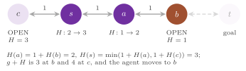
4.13 Hierarchical path-finding¶
On a map that is searched many times, with different starts and goals,
one can pay once for an abstraction of the map and then answer each
query with a search of the abstract graph and of two small parts of the
map. This is Hierarchical Path-Finding A\(^*\) (HPA\(^*\)) of Botea, Müller
and Schaeffer [120], which
HPAStar< Moves > (HPAStar.h) implements with one level of
abstraction on a GridMap with 4 or 8 moves. The map is split in clusters of
\(C \times C\) cells. Along the border of two adjacent clusters, every maximal
run of pairs of free cells facing each other is an entrance, which gets a
transition, i.e., a pair of abstract nodes, one on each side, joined by
the move between them, in its middle if the run is shorter than the
split length, and one at each end otherwise. Inside a cluster, its
abstract nodes are joined by the shortest paths that stay in the
cluster, computed once by the algorithm of Dijkstra and kept with the
edges. A query inserts the start \(s\) and the goal \(t\) into the abstract
graph, joined to the abstract nodes of their clusters by the shortest
paths inside them, searches it with A\(^*\) on the distance of the Grid,
and refines the abstract path by concatenating the paths kept; when \(s\)
and \(t\) are in the same cluster, the shortest path inside it is a
candidate too, and the abstract search stops as soon as the node
selected has a \(g\) not smaller than that candidate. The path is then
smoothed as in [120]: from each of its
cells, a straight walk in each of the directions of the moves that meets
a later cell of the path replaces the piece between them if it costs
less, so that the detours through the transitions are cut. The options
are
struct HPAOptions {

 int cluster = 10;            ///< the side C of a cluster
 int split = 6;               ///< the entrances at least this long get two
                              ///< transitions
 bool smooth = true;          ///< the path is smoothed [see HPAStar]

 };  // end( struct( HPAOptions ) )
and the declarations, quoted by hand, are
template< int Moves = 4 >
class HPAStar {
 public:
 explicit HPAStar( const GridMap & map , const HPAOptions & options = {} );
 [[nodiscard]] std::size_t nodes( void ) const noexcept;
 [[nodiscard]] std::size_t edges( void ) const noexcept;
 [[nodiscard]] std::uint64_t preprocessing( void ) const noexcept;
 [[nodiscard]] Solution< typename Grid< Moves >::state_type ,
                         typename Grid< Moves >::cost_type >
  solve( int sx , int sy , int gx , int gy ) const;
 };
where a state is the index of a cell and the cost is an integer with 4
moves and a double with 8. The
constructor builds the abstract graph, and throws
std::invalid_argument if the map has no free cell or the side of a
cluster is not positive; nodes() and edges() give its size and
preprocessing() the expansions of its searches of Dijkstra. The query
solve( sx , sy , gx , gy ) throws std::invalid_argument if the start
or the goal is blocked, and returns the path with the counters of the
insertion of \(s\) and \(t\) and of the abstract search in expanded and
generated.
Proposition 4.29 (What HPA\(^*\) returns). (i) Before the smoothing, the path of a query is a cheapest one among the abstract paths, i.e., the concatenations of a shortest path inside the cluster of \(s\) from \(s\) to one of its abstract nodes, of abstract edges, and of a shortest path inside the cluster of \(t\) from one of its abstract nodes to \(t\), together with the shortest path inside the cluster when \(s\) and \(t\) share it. (ii) The smoothing does not increase the cost, and the cost returned is that of the path returned, which is a path of the grid; hence it is at least \(C^*\). (iii) The search is not complete: a query may fail although \(t\) is reachable from \(s\).
Proof. (i) The distance of the Grid (Manhattan or octile, times the least cost of a free cell) is consistent on the grid (Chapter 14), and an abstract edge costs as a path of the grid between its ends; hence the heuristic is consistent on the abstract graph, by the triangle inequality along that path, and the abstract A\(^*\) selects the goal with the least cost of an abstract path (Theorem 2.13). When it stops early, the node selected has \(f \ge g \ge\) the candidate, and every abstract path not yet found costs at least the least \(f\) of OPEN, so that the candidate is not worse. (ii) A piece is replaced only by a walk of moves that the grid allows (a blocked cell or a cut corner ends the walk) and only if the walk costs less; the cost is then summed again over the moves of the final path. (iii) A transition is placed in the middle or at the ends of an entrance, and when a cluster is disconnected inside, a cell of an entrance may be reachable within its cluster while the cell of its transition is not; then the abstract graph lacks a connection that the map has, as in the original method. \(\square\)
The path is therefore not optimal in general, since it goes through the
transitions; the test hpa checks on four random maps of \(64 \times 64\)
cells, with clusters of 8 and 16 cells, that the paths are valid paths of
the grid and never cheaper than those of A\(^*\), that at least 90% of the
queries that A\(^*\) solves are solved, and that the worst ratio to the
cost of A\(^*\) is below 1.5 with 8 moves, together with a query from the
goal and one inside a single cluster, which is optimal. The query costs a
search of the abstract graph and of two clusters instead of a search of
the map, which is the point of the method.
4.14 Baselines: breadth-first and cost-bounded depth-first search¶
Two searches of the library serve as baselines, against which the
others are measured. BreadthFirst (BreadthFirst.h) is the
breadth-first search of a Domain with duplicate detection, which
ignores both the costs and the heuristic, with the goal test at the
generation.
Algorithm 4.13 (Breadth-first search, the pseudocode of the header).
 1  procedure BFS(s₀)
 2     if s₀ is a goal then return the path (s₀)
 3     CLOSED ← {s₀};  L ← (s₀)
 4     while L ≠ ∅ do
 5        L' ← ()
 6        for each u of L, in order, do
 7           for each successor v ∉ CLOSED of u do
 8              add v to CLOSED, with parent(v) ← u
 9              if v is a goal then return the path to v
10              append v to L'
11        L ← L'
12     return unsolvable
The layers \(L\) and \(L'\) are two vectors of nodes and CLOSED is a
NodeTable; the heuristic is computed by the domain only because the
successors come with it. The declarations, quoted by hand, are
template< Domain D >
class BreadthFirst {
 public:
 explicit BreadthFirst( const D & domain ,
                        const SearchOptions & options = {} );
 [[nodiscard]] Solution< state_t< D > , cost_t< D > > solve( void ) const;
 };

template< Domain D >
[[nodiscard]] Solution< state_t< D > , cost_t< D > >
breadth_first( const D & domain , const SearchOptions & options = {} );
with node_limit on the nodes of CLOSED, tested after each expansion,
and expected_nodes sizing CLOSED. The search stops at the first goal
generated, but the domain gives all the successors of its parent, and
those that follow the goal are counted in generated without being
looked up or stored.
Proposition 4.30 (Breadth-first search).
Algorithm 4.13 returns a path with the least number of edges to a goal,
of cost the sum of its edges, which is the least cost when all the edges
cost the same; on a finite graph it terminates, and returns
unsolvable if no goal is reachable.
Proof. By induction on \(d\), the layer \(L\) of the iteration \(d\) holds exactly the states at the least depth \(d\) that are not goals, and CLOSED those at depth at most \(d\) and, at the end of the iteration, those at depth \(d + 1\) generated so far: a state at least depth \(d + 1\) is a successor of a state at depth \(d\), which is in \(L\), and it is not in CLOSED before, since it is not at a smaller depth. The first goal generated is therefore at the least depth, and its path through the parents has that number of edges, the parents being set once. On a finite graph each state enters a layer at most once. \(\square\)
The test bfs checks the costs on 21 states of the 8-puzzle, against
their exact distances, the path of fewest edges of the map of Romania
from Arad (Arad, Sibiu, Fagaras, Bucharest, of cost 450, not the
cheapest one, of cost 418), the proof that a grid split by a wall is
unsolvable, and the edge cases of A\(^*\) (a start that is a goal, a start
one move away, and the node limit). The cost-bounded depth-first
search cost_bounded_dfs( domain , bound , options ) is one iteration
of IDA\(^*\) with the bound \(\beta\) given, i.e., the first call of line 5
of Algorithm 4.3 with that \(\beta\) and no other (it calls
IDAStar::solve( bound ), with the bound on \(f'\) if the options have a
weight).
Proposition 4.31 (The cost-bounded
depth-first search). Let the costs be at least some \(\varepsilon > 0\)
and the branching finite. The search terminates, and it returns a path
whose nodes have \(f \le \beta\), hence of cost at most \(\beta\), if it
finds one; if \(h\) is admissible, it finds one whenever \(\beta \ge C^*\),
and it returns unsolvable whenever \(\beta < C^*\).
Proof. The iteration visits only paths whose nodes have \(g \le f \le \beta\), i.e., with at most \(\beta / \varepsilon\) edges, finitely many. The goal entered has \(g = f \le \beta\) (its \(h\) being 0 if \(h\) is admissible, and in any case \(g \le g + h \le \beta\)). If \(\beta \ge C^*\), an optimal path whose moves are all kept has every node within the bound, and the iteration, which visits every path of its tree within the bound unless it enters a goal before, enters its goal or another one. If \(\beta < C^*\), a goal entered would have \(g \le \beta < C^*\), which no path has. \(\square\)
The path need not be optimal when \(\beta > C^*\): the test bfs checks
that the search at the cost of two instances of the 15-puzzle of Korf
finds a path of that cost and one less finds none, that on the map of
Romania the bound 450 gives a path of cost between 418 and 450 and the
bound 417 none, and the bound 0 at a goal and one move away.
4.15 Benchmark¶
Our benchmark of this chapter compares the searches that are optimal
with an admissible heuristic and keep less than A\(^*\), or spend less per
node, with A\(^*\) on the same instances: IDA\(^*\) and IDA\(^*\)-CR, RBFS,
PEA\(^*\) and EPEA\(^*\), fringe search and DDD-A\(^*\) on the 100 instances
of the 15-puzzle of Korf [7] with the
Manhattan distance, and IDA\(^*\)-CR, PEA\(^*\), EPEA\(^*\) and fringe search
on the grids of [15], where the values of \(f\)
are many and the iterations of IDA\(^*\) are a burden. The measures are
those of §2.16: each instance is solved in a
process of its own, pinned to one core, with the clock of the search
only, and the counters of the Solution are machine-independent.
Table 4.1. The memory-bounded searches against A\(^*\): for each search and set of instances, the instances solved, the seconds summed over the instances (each the median of its repetitions), the nodes expanded and the nodes stored summed over the instances, and the millions of expansions per second.
| search | instances | solved | seconds | expanded | stored | expansions per second (millions) |
|---|---|---|---|---|---|---|
Placeholder: the results of this table are to be measured on an idle machine and written here by manual/build/tables.py; no number is given until then.
4.16 An example¶
The following example, a case of the tester, solves an instance of the
15-puzzle of Korf with IDA\(^*\), whose memory is the path, and with
DDD-A\(^*\) on 16 files per bucket and small buffers in a directory of its
own; it checks the costs, the counter stored of IDA\(^*\) (Proposition
4.8), that DDD-A\(^*\) expands each state at most once
(Theorem 4.15), that no file is left behind, and that
IDA\(^*\) stops at a limit of 1000 expansions.
const FifteenPuzzle d( ki.board );
const auto i = idastar( d );                  // memory: the path only
DDDOptions x;
x.partitions = 16;              // files per bucket (default 64)
x.buffer_bytes = 1 << 12;       // buffer of each file written (2^16)
x.directory = dir.path();       // if empty, the temporary of the system
const auto e = ddd_astar( d , SearchOptions{} , x );
// the node limit bounds the expansions of IDA*, the states closed by
// DDD-A*
SearchOptions lim;
lim.node_limit = 1000;
const auto l = idastar( d , lim );
4.17 Notes and references¶
DFID and IDA\(^*\) are due to Korf [7], who proved that DFID is asymptotically optimal among the brute-force tree searches in time and space, and IDA\(^*\) with a disjoint pattern database is the search of Korf and Felner [22] on the 24-puzzle; RBFS is also due to Korf [116], the transposition tables in iterative deepening were studied by Reinefeld and Marsland [161], and the stochastic node caching by Miura and Ishida [162]. The External A\(^*\) is that of Edelkamp, Jabbar and Schrödl [39], the hash-based DDD that of Korf [40], applied by Korf and Schultze to the complete breadth-first search of the 15-puzzle [156], and the two-bit breadth-first search that of Korf [26]. The BDDs are due to Bryant [163], and the symbolic search with them and the beam search are surveyed by Edelkamp and Schrödl [10], the breadth-first beam search going back to Lowerre [171] and the beam that keeps its dropped nodes in CLOSED, with its complete variant by backtracking, to Zhou and Hansen [117]; the width-based search is due to Lipovetzky and Geffner [104]. Partial expansion is due to Yoshizumi, Miura and Ishida [42], its enhanced form with the operator selection function to Felner et al. [113] and Goldenberg et al. [114], fringe search to Björnsson, Enzenberger, Holte and Schaeffer [115], the controlled bounds of IDA\(^*\)-CR to Sarkar, Chakrabarti, Ghose and De Sarkar [132], LRTA\(^*\) to Korf [118], LSS-LRTA\(^*\), with the proofs of admissibility and convergence that we cite in §4.12, to Koenig and Sun [119], and HPA\(^*\) to Botea, Müller and Schaeffer [120]; the moves that a tree search of Rubik's cube need not try are those of Korf [59].
As to where the library stands, the following facts are stated from the
code. IDAStar is the algorithm of [7] with
the test of the bound at the generation and the parent pruning of
§2.9, and it runs with the pattern
databases of Chapter 5 on the 24-puzzle (the
README reports, for 50 ends of random walks of 150 moves, 49 instances
solved within \(10^{10}\) expansions each, a count that does not depend on
the machine). DDDAStar uses the hash-based detection rather than the
sorting of [39], but it keeps all the closed
files and does not implement the frontier search, nor a parallel
expansion of the files as in [156]; its order
by increasing \(g\) within a layer may cost many more expansions than
A\(^*\) in the last layer. BeamSearch keeps the dropped nodes in CLOSED,
which bounds its memory only by the depth, and has no beam stack;
RBFS and FringeSearch follow the methods of
[116] and [115], the
latter with the cache of \(g\) and the insertion of the children after
their parent that make it the depth-first order of IDA\(^*\); PEAStar
adds to [42] the skip of the known
successors of Lemma 4.20 and the slack of the real costs,
and EPEAStar relies on an operator selection function written for each
domain, which the sliding-tile puzzles and the grids provide; IDAStar
takes the bounds of IDA\(^*\)-CR from a histogram of binary exponents,
adds the doubling of the step of §4.11 for the iterations
that grow slowly, and completes the iteration of the first goal as a
branch-and-bound; RealTimeSearch runs the trials of LRTA\(^*\) and
LSS-LRTA\(^*\) on any Domain, with the update by the algorithm of
Dijkstra of [119]; HPAStar has one level
of abstraction and the smoothing of [120],
and works on the grids only. The depth-first branch-and-bound of a
Domain, the transposition tables and the stochastic node caching of
IDA\(^*\), and the symbolic search are not in the library.
4.18 Exercises¶
Exercise 4.1 (discussion, no test). On a grid with 8 moves, when any path to the goal will do and its length does not matter, is depth-first branch-and-bound a good choice? Compare it with a greedy best-first search by \(h\) and with A\(^*\), and consider what happens to the incumbent \(U\) and to the paths that reach the same cell.
Exercise 4.2 (ctest -R PBeFS.idastar). IDA\(^*\) usually expands
more nodes per second than A\(^*\) on the 15-puzzle. Explain why from
Algorithm 4.3 and the structures of Chapter
3 (what each expansion touches in memory),
and use the counters expanded and stored of the Solution of both
on the instances of the test to compare the work and the memory.
Exercise 4.3 (discussion, no test). With a branching factor of 4
and a number of nodes that grows by that factor per level, an external
search that can store 1000 times more nodes than A\(^*\) reaches a depth
larger by how much? Show that the answer is \(\log_4 1000\), i.e., about
5 levels, and discuss what this means for DDDAStar.
Exercise 4.4 (ctest -R PBeFS.tiles24). Which of the searches of
this chapter would you choose for problems whose solutions are deeper
still, if the time were unlimited but the memory were not? Argue from
the memory of each (Propositions 4.8, 4.11 and 4.16), and look at how
the test runs IDA\(^*\) with a pattern database on the 24-puzzle.
Exercise 4.5 (ctest -R PBeFS.idastar). Prove the bound \((C^* -
h(s_0)) / 2 + 1\) on the iterations of IDA\(^*\) on the sliding-tile
puzzles with the Manhattan distance (Proposition 4.7) in
detail, i.e., prove that a move changes the Manhattan distance by
exactly 1, and check on the instances of the test that stored equals
\(C^* + 1\) (Proposition 4.8).
Exercise 4.6 (ctest -R PBeFS.idastar). Show that IDA\(^*\) reports
the acyclic graph of the test unsolvable, and build a graph of three
states with a cycle and no goal on which it does not terminate without
the node limit; what is the sequence of its bounds?
Exercise 4.7 (ctest -R PBeFS.ddd). Prove in detail the identity
\(\mathit{generated} + 1 = \mathit{stored} + \mathit{duplicates}\) for a
search of DDDAStar that ends without a goal, and that expanded \(=\)
stored \(= 1250\) on the grid with the wall of the test.
Exercise 4.8 (ctest -R PBeFS.ddd). Build a graph with an
admissible but inconsistent heuristic on which the order of the buckets
of DDD-A\(^*\) would close a state with a \(g\) larger than its optimal one,
and explain why DDDAStar refuses such a heuristic rather than reopening
the state (the test runs it on the inconsistent graph of the test
reopen).
Exercise 4.9 (discussion, no test). Give an example in which the transposition table of Proposition 4.10 makes IDA\(^*\) skip a value of the bound, and show that the search still returns an optimal path; how many iterations does it save on your example?
Exercise 4.10 (ctest -R PBeFS.ddd). IDAStar bounds with
node_limit the expansions, while DDDAStar bounds the states written
to the closed files. Explain why each choice measures the resource that
the search consumes, and check how the two tests stop the searches at
their limits.
Exercise 4.11 (ctest -R PBeFS.classic). Run PEA\(^*\) with \(C = 0\)
by hand on a node whose successors have \(f = 5, 5, 7, 9\), as in
Figure 4.9, and count its selections; then do the same with
EPEA\(^*\) and count the successors generated. Show that with \(C = 2\) the
node is selected twice, and explain why the test checks that PEA\(^*\) with
\(C = 2\) is still optimal on 200 states of the 8-puzzle
(Theorem 4.21).
Exercise 4.12 (ctest -R PBeFS.classic). Build a graph with an
admissible heuristic and an edge of \(\Delta f < 0\) on the only optimal
path, and show that EPEA\(^*\) with an operator selection function that
follows its definition misses that path, whereas PEA\(^*\) does not. Which
hypothesis of Theorem 4.21 fails, and why do the domains of
the test (the puzzles with the Manhattan distance, the grids with the
octile distance) satisfy it?
Exercise 4.13 (ctest -R PBeFS.classic). Prove that fringe search
and IDA\(^*\) have the same thresholds on a tree, i.e., when no state is
reached by two paths, and that on a graph the cache of fringe search may
only skip expansions. Then show why the test runs RBFS on grids of only
\(8 \times 8\) cells, by counting the paths of Figure 4.4
that RBFS follows below a bound.
Exercise 4.14 (ctest -R PBeFS.classic). In the proof of
Proposition 4.11, where is the absence of a cycle on the
optimal path used? Give a domain with a cycle of cost 0 on which the
proof would fail as written, and repair it by choosing the path.
Exercise 4.15 (ctest -R PBeFS.classic). Prove that the beam
search of infinite width returns the cost of the shortest path on the
8-puzzle, whose costs are uniform, and give a graph with nonuniform
costs on which the cost returned differs from the cost of the path
rebuilt from the parents (cf. the remark after
Proposition 4.2).
Exercise 4.16 (ctest -R PBeFS.idastar). On a grid with 8 moves,
whose diagonal moves cost \(\sqrt 2\) times the straight ones, show that
the classical bounds of IDA\(^*\) may be as many as the values of \(f\)
below \(C^*\), and that the bounds of IDA\(^*\)-CR with \(r = 2\) are fewer.
With optimal false, compute the bound of
Proposition 4.26 on an example, and check that the test
compares the first path with the optimum.
Exercise 4.17 (ctest -R PBeFS.idastar). Show that the
branch-and-bound of Proposition 4.26 (ii) ends with the
optimum even if its iteration has a bound much larger than \(C^*\), and
estimate how many nodes it enters in that case against an iteration of
bound \(C^*\). Why does the code not prove the optimality when the node
limit stops that iteration?
Exercise 4.18 (ctest -R PBeFS.realtime). Run LRTA\(^*\) by hand on a
path of four states with unit costs and \(h = 0\), and list the values of
\(H\) after each move of the first trial and of the second; show that
they stay below \(h^*\) (Theorem 4.28) and that the second
trial costs the optimum. The test checks the convergence and the
admissibility on random grids for the lookaheads 1 to 64.
Exercise 4.19 (ctest -R PBeFS.realtime). Prove that with a
lookahead \(L\) at least the number of the states reachable from \(s_0\),
the first trial of LSS-LRTA\(^*\) is an A\(^*\) from \(s_0\) followed by the
moves of an optimal path, and therefore costs \(C^*\) when \(h\) is
consistent.
Exercise 4.20 (ctest -R PBeFS.hpa). Draw a cluster whose free
cells form two parts, such that the cell of the transition of an
entrance is in one part and the start in the other, and show that
HPA\(^*\) fails on a query that A\(^*\) solves (Proposition
4.29 (iii)). How does the test allow for such failures?
Exercise 4.21 (ctest -R PBeFS.hpa). Show that a query whose start
and goal are in the same cluster of an empty map is answered at the
optimal cost, as the test checks for the cells \((1, 1)\) and \((4, 5)\) of
a map of \(20 \times 20\) cells (cost 7), and give an example in which the
abstract path is cheaper than the path inside the cluster.
Exercise 4.22 (ctest -R PBeFS.bfs). On the map of Romania, show
that breadth-first search returns Arad, Sibiu, Fagaras, Bucharest, of
cost 450, while the cost-bounded depth-first search with the bound 450
may return a path of cost between 418 and 450 (Proposition
4.31); which path does it return with the straight-line
distance and the order of the roads of the test?
Exercise 4.23 (ctest -R PBeFS.rubik). Prove that skipping, after a
turn of a face of Rubik's cube, the turns of the same face and, after a
turn of the second face of a pair of opposite faces, those of the first,
keeps a path of the same end and of the same length for every path, as
TreeOperatorDomain requires, and derive the counts 18 and 243 of the
first two depths of the tree that the test checks.