9. Hash-distributed search¶
[Source: include/PBeFS/astar/HDAStar.h (HDAStar,
ParallelOptions), include/PBeFS/astar/HDAStarMPI.h
(HDAStarMPI), include/PBeFS/astar/Distribution.h (the
work distributions), include/PBeFS/astar/Domain.h
(FeatureDomain, IncrementalFeatureDomain, AbstractFeatureDomain,
AbstractStateDomain, PerfectHashDomain),
include/PBeFS/core/SearchUtils.h (ParallelParams)]
We are concerned in this chapter with Hash Distributed A\(^*\) (HDA\(^*\))
of Kishimoto, Fukunaga and Botea [2], the
parallel search in which each state has an owner among the \(p\)
workers, fixed by a function of the state alone. Only the owner stores
the state; hence, the workers share no OPEN and no CLOSED list, and yet
the duplicates are detected as in the sequential search. In the
searches of Chapter 8 (from the Parallel
A\(^*\) with one shared OPEN list onwards) each node costs a lock, or an
atomic operation, on a structure that all the workers touch. HDA\(^*\)
replaces them by messages between pairs of workers, at the price of the
nodes that change worker and of an order of expansion that is only (and
often rather loosely) that of A\(^*\). We use the notation of
Chapter 1 and the invariants of A\(^*\) of
Chapter 2; the search overhead (SO), the
communication overhead (CO) and the load balance (LB) of a parallel
search, and the general question of when a parallel search may stop,
are those of Chapter 8. The structure
of the chapter is as follows. §9.1 states the interface
(the search, its options, the concept of a distribution and the
refinements of the Domain that the distributions need),
§9.2 gives the algorithm with its invariants, the proof
of its optimality and the cost of its steps, and §9.3 the
mailbox through which the messages travel, with the proof that it
detects the end without error. §9.4 and §9.5 are
devoted to the distributions and to the incremental Zobrist hash,
§9.6 to the search over MPI with the termination detection
of Mattern, and §9.7 to the engineering of the
implementation; the chapter ends with the benchmark, the notes and the
exercises.
9.1 The search and its interface¶
A search is an object of the class template HDAStar, built from a
Domain D, a distribution Dist and the options, and run by
solve(), which returns the Solution (the status, the cost, the path
and the counters of Chapter 2); the following
declarations are quoted from HDAStar.h:138-188, where
they come with their bodies.
template< Domain D , class Dist = StateHashDistribution< D > ,
          WorkerExecutor Executor = ThreadPool ,
          class Open = /* buckets for integer costs, a heap otherwise */ >
class HDAStar {
 public:
 HDAStar( const D & domain , const Dist & dist ,
          const ParallelOptions & options = {} );   // both must outlive it
 void set_executor( Executor & ex ) noexcept;
 [[nodiscard]] Solution< state_t< D > , cost_t< D > > solve( void ) const;
 };
Its workers run on an Executor, i.e., on a pool of C++ threads (the
default), on OpenMP or on FastFlow [12]
(§1.6). One can give the search an
executor that outlives it by set_executor(), which saves the start of
the threads at each search; otherwise, solve() builds one of \(p\)
threads. The options are a ParallelOptions, i.e., the options of the
sequential search plus the parameters of the parallel ones
(SearchUtils.h:98-115): the number \(p\) of workers
(threads, 1 by default), the number of nodes packed in a message (batch,
64), the number of expansions between two flushes of the outboxes that are not
full (flush_period, 64) and a seed, which HDAStar does not read (a
distribution takes its seed in its constructor, 1 by default). A
parameter equal to 0 is taken as 1 (normalize()), and therefore no
setting of the options can stop the exchange of the nodes. The
following example, from the case manual of the tester, which the
build compiles and runs (ctest -R PBeFS.manual), solves an instance of
the 8-puzzle of optimal cost 26 with Zobrist hashing and with Abstract
Zobrist hashing (§9.4) on 4 workers and reads the counters
of §8.2:
const EightPuzzle d( EightPuzzle::parse( "7 2 4 5 0 6 8 3 1" ) );
ParallelOptions o;
o.threads = 4;
o.batch = 64;           // nodes per message (the default)
o.flush_period = 64;    // expansions between two flushes of an outbox
// the seed changes the owners of the states, not the cost
const ZobristDistribution< EightPuzzle > z( d , 7 );
const auto a = HDAStar< EightPuzzle , decltype( z ) >( d , z , o )
               .solve();
const AbstractZobristDistribution< EightPuzzle > az( d );
const auto b = HDAStar< EightPuzzle , decltype( az ) >( d , az , o )
               .solve();
const double co = a.stats.communication_overhead();  // sent / generated
const double lb = a.stats.load_balance();
const auto sent = a.stats.sent;           // nodes sent to another worker
const auto messages = a.stats.messages;   // the batches they went in
The same search with one MPI process per worker is
template< Domain D , class Dist = StateHashDistribution< D > >
class HDAStarMPI {
 public:
 HDAStarMPI( const D & domain , const Dist & dist ,
             const ParallelOptions & options = {} ,
             MPI_Comm comm = MPI_COMM_WORLD );
 [[nodiscard]] Solution< state_t< D > , cost_t< D > > solve( void ) const;
 };
(HDAStarMPI.h:111-144), described in
§9.6; there threads is not read, the number of workers being that
of the processes of the communicator.
The distributions¶
A distribution is a class with a method owner( s , p ) that returns
the worker in \(\{0, \ldots, p - 1\}\) which owns the state \(s\), and with
a static method name() that gives its name in the notation
\(\mathrm{HDA}^*[\mathit{hash}, \mathit{abstraction}]\) of Jinnai and
Fukunaga (section 2.6 of [5]). Each
distribution of the library has a constructor that takes the Domain
and a seed, e.g.,
template< FeatureDomain D >
class ZobristDistribution {
 public:
 explicit ZobristDistribution( const D & domain , std::uint64_t seed = 1 );
 [[nodiscard]] std::uint64_t hash( const state_t< D > & s ) const;
 [[nodiscard]] std::uint32_t key( const state_t< D > & s ) const;
 [[nodiscard]] unsigned owner( const state_t< D > & s , unsigned p ) const;
 [[nodiscard]] std::uint32_t key( std::uint32_t k , const state_t< D > & s ,
                                  const state_t< D > & t ) const
  requires IncrementalFeatureDomain< D >;
 [[nodiscard]] static std::string name( void );
 };
(Distribution.h:134-187, declarations quoted
without their bodies). We remark that the search on a shared memory requires no
more of a distribution; in particular, the owner need not be deterministic
there (the random distribution of §9.4 is not), and each worker
keeps a copy of the distribution, so that a distribution with a
mutable state (the generator of the random one) needs no lock.
HDAStarMPI, on the contrary, needs a deterministic owner, since it
rebuilds the path by asking the owner of each state
(§9.6). A distribution that can follow the moves models the
concept IncrementalDistribution (Distribution.h:631):
it also gives a 32-bit key key( s ) (for Zobrist hashing, the high 32 bits
of the hash of §9.4), whose owner among \(p\) workers is
key_owner( key( s ) , p ), and the key key( k , s , t ) of a
successor \(t\) of \(s\) computed from the key \(k\) of \(s\), which must equal
key( t ). HDA\(^*\) keeps the key of each node in the node, and the
function successor_owners() (Distribution.h:660)
returns, for the node being expanded, a function that maps each successor to
its owner and its key, computed from the key of the parent when the
distribution is incremental and from scratch otherwise (the key is then 0, as
distribution_key() returns for a distribution that is not
incremental).
What the distributions need from the Domain¶
Each distribution requires of the Domain the least that it uses, through
a refinement of the concept Domain of
Chapter 1 (all in Domain.h).
FeatureDomain(Domain.h:193): a state is a set of propositions, the features, taken from a universe ofnum_features()of them, andfor_each_feature( s , f )callsf( i )for each feature \(i\) that holds in \(s\). Zobrist hashing needs it.IncrementalFeatureDomain(Domain.h:209): moreover,for_each_feature_change( s , t , f )callsf( i )for each feature that holds in exactly one of \(s\) and of its successor \(t\), i.e., for the features of the symmetric difference of the two sets.AbstractFeatureDomain(Domain.h:221): moreover, a projectionabstract_feature( i )of the features ontonum_abstract_features()abstract features, which is the projection \(A\) of Abstract Zobrist hashing.AbstractStateDomain(Domain.h:267): a mapabstract_state( s )of the states to the integers, i.e., a state abstraction.PerfectHashDomain(Domain.h:408): an injective mapperfect_hash( s )of the states to the integers.
On the sliding-tile puzzles (SlidingTile.h:395-480)
a feature is a pair (tile, cell), i.e., the index \(t \cdot n + c\) for the tile
\(t \ne 0\) in the cell \(c\) of a board of \(n\) cells. An abstract feature
is a pair (tile, half of the board), the half being the top rows or the
bottom rows, and the abstract state of a state is the triple of the
cells of the tiles 1, 2 and 3, which is the abstraction that Jinnai and
Fukunaga chose among the candidates of footnote 4 of section 3.1.4 of
[5]. Furthermore, the grids and the vacuum
world give features and abstractions as well (cf. Chapter
14), and any Domain gives the hash of its closed
list, which is all that the default distribution needs (one can
therefore run HDA\(^*\) on any Domain).
Two more refinements, FeatureGroupDomain and
FeatureTransitionDomain, give the groups of the features and the
transitions between them, which the automatic distributions read
(Definition 10.2), and LevelDomain
gives the levels of the hyperplane distribution
(Chapter 15).
9.2 Hash Distributed A\(^*\)¶
We now describe the search. Each worker \(i\) runs A\(^*\) on its lists \(\mathrm{OPEN}_i\) and \(\mathrm{CLOSED}_i\), which hold only the states \(v\) with \(\mathrm{owner}(v) = i\). A successor generated by a worker is sent to its owner, which checks it against its CLOSED list and possibly inserts it in its OPEN list, as the sequential A\(^*\) does with a state that it generates. The incumbent \(z\), i.e., the cost of the best goal found so far, is shared by the workers, and each node with \(f \ge z\) is pruned. We write a message as \((v, g', u)\): it carries a state \(v\) with the cost \(g'\) of the path that reached it and its predecessor \(u\) on that path (and, in the implementation, the operator that generated \(v\), its heuristic and its key).
Algorithm 9.1 (HDA\(^*\)).
 1  procedure HDA*(s₀, p, owner)
 2     z ← ∞;  INSERT(s₀, 0, nil) on owner(s₀)
 3     in parallel, on each worker i = 0, ..., p − 1 do
 4        while the search is not over do
 5           for each message (v, g', u) received do INSERT(v, g', u)
 6           if OPEN_i has a node of f < z then
 7              u ← the first node of OPEN_i, removed (stale entries
                   dropped);  close u
 8              if u is a goal then
 9                 z ← min(z, g(u)), recording u if g(u) < z
10              else for each successor v of u do
11                 g' ← g(u) + c(u, v)
12                 if g' + h(v) ≥ z then continue
13                 if owner(v) = i then INSERT(v, g', u)
14                 else send (v, g', u) to owner(v)
15              every k expansions, send the outboxes not yet full
16           else
17              send all the outboxes;  wait for mail or for the end
18     return the path to the goal of cost z, if z < ∞
19  procedure INSERT(v, g', u)                       ▷ on the owner i of v
20     if g' + h(v) ≥ z then return
21     if v ∉ CLOSED_i then
22        add v to CLOSED_i, with g(v) ← g' and parent(v) ← u
23     else if g' < g(v) then
24        g(v) ← g';  parent(v) ← u;  v is not closed
25     else return                                         ▷ a duplicate
26     push (g' + h(v), g', v) in OPEN_i
This is the pseudocode of HDAStar.h:18-46. We comment on
the lines that are not those of A\(^*\).
- Line 2: the root is inserted by its owner before the first expansion, and the other workers start with empty lists and wait for mail; the first expansions are therefore those of a single worker, which is the initial burst of the search (section 3.1.2 of [5]).
- Line 5: the messages are processed before each expansion; hence, a cheaper path that has arrived is used at once.
- Line 7: CLOSED holds all the nodes that a worker has stored, closed or not, and OPEN is a priority queue of entries with lazy deletion: when the \(g\) of a node decreases (line 24) a new entry is pushed, and the old one becomes stale and is dropped when it reaches the top, as in the sequential search (§3.1).
- Lines 8 and 9: the goal test is made at the expansion, not at the generation, and therefore a goal is recorded only when it is the best node of its owner; the incumbent is an atomic variable, and the goal is recorded under a mutex.
- Lines 12 and 20: a node with \(f \ge z\) is pruned twice, by the worker that generates it (which saves the message) and by its owner (since \(z\) may have decreased while the node was travelling).
- Lines 13 and 14: a successor owned by the expanding worker does not go
through the mailbox, while one owned by another worker is appended to
the outbox of that worker, which leaves as one message when it holds
batchnodes (cf. §9.3). - Lines 15 and 17: an outbox that is not full leaves after each block of
flush_periodexpansions, and all the outboxes leave before the worker waits; the wait ends when mail arrives or when the mailbox detects the end of the search, i.e., when no worker has a node of \(f < z\) and no node is travelling (§9.3). - Line 18: the parents cross the workers (a node records a pointer to the node of its predecessor, which may belong to another worker), and they are followed only after all the workers have returned.
As the sequential search, HDA\(^*\) skips the move back to the parent in
an OperatorDomain: the operator that generated a state travels in its
message, and the successor that the inverse operator leads to is never
generated, since it is never cheaper than the parent (cf.
§2.9); on the sliding-tile puzzles this
typically saves about one successor out of three and, in HDA\(^*\), its
message as well.
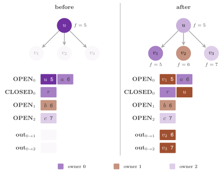
Figure 9.1 shows an expansion. The code runs the loop of a worker as follows, with the operations SEND, FLUSH, POLL, QUIESCENT and STOP of the mailbox of §9.3 (Algorithm 9.3): the inbox is drained as a whole, and the hashes of all its nodes are computed and their places in the closed list prefetched before the first lookup, so that the cache misses of the lookups overlap instead of following one another (§3.8), and the owners of the successors are computed from the key of the parent (§9.5).
Algorithm 9.2 (The loop of a worker of HDA\(^*\), as coded).
 1  procedure WORKER(i)
 2     if i = owner(s₀) then INSERT(s₀, 0, nil)
 3     k ← 0
 4     while the mailbox is not stopped do
 5        M ← POLL(i)                               ▷ the whole inbox
 6        for each (v, g', u) ∈ M do                ▷ phase 1
 7           compute the hash of v;  prefetch its place in CLOSED_i
 8        for each (v, g', u) ∈ M do INSERT(v, g', u)        ▷ phase 2
 9        u ← NEXT()
10        if u ≠ nil then
11           EXPAND(u);  k ← k + 1
12           if k = flush_period then k ← 0;  FLUSH(i)
13           if i stores node_limit nodes then the limit is hit;  STOP()
14        else if QUIESCENT(i) then return
15        else wait a little
16  function NEXT()
17     while OPEN_i is not empty do
18        (f, γ, u) ← the first entry of OPEN_i
19        if it is stale then remove it;  continue
20        if f ≥ z then return nil
21        remove it;  return u
22     return nil
23  procedure EXPAND(u)
24     close u
25     if u is a goal then
26        lock the goal record
27        if g(u) < z then z ← g(u);  record u
28        unlock the goal record;  return
29     O ← the map of the successors to their owners, from the key of u
30     for each successor v of u not reached by the inverse operator do
31        g' ← g(u) + c(u, v)
32        if g' + h(v) ≥ z then continue
33        j ← the owner given by O(v)
34        if j = i then INSERT(v, g', u)
35        else SEND(i, j, (v, g', u))
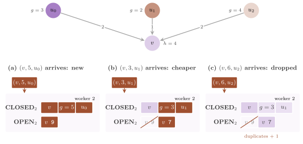
Figure 9.2 shows what the owner of a state does with the copies of it that the other workers send. All the copies of \(v\) reach the same worker, which keeps in its CLOSED list the cheapest of those that it has processed. Hence, the duplicate detection is that of the sequential search. The difference is that the copies arrive in an order that depends on the timing of the workers, and a copy that arrives after its state has been expanded with a larger \(g\) reopens it. This is why HDA\(^*\) may reopen a state even when the heuristic is consistent (footnote 6 of section 3 of [2]; one can build a small example, cf. Exercise 9.5), and the reopenings are part of its search overhead.
Invariants¶
We now state the invariants of Algorithm 9.1, from which its optimality follows. We assume that the costs are nonnegative and the heuristic is admissible, as in Chapter 2, and \(C^*\) is the cost of an optimal path from \(s_0\) to a goal. The first invariant is the reason why the workers need no lock on the nodes.
Lemma 9.1 (Ownership). At any time, each node is created, stored and written only by the worker that created it, which is the owner of its state for the copy of the distribution of that worker; if the distribution is deterministic, at most one node of \(v\) exists, at \(\mathrm{owner}(v)\), and each copy of \(v\) that is generated is compared with it.
Proof. A node is created only by INSERT (lines 21-22), which a worker calls only on a state that it owns: either on the root, by its owner (line 2), or on a message, which was sent to the owner of its state (line 14), or on a successor that it owns (line 13). A node is written by INSERT (lines 22-24) and by the expansion (line 7), and a worker expands only the nodes of its OPEN list, which INSERT fills. The other workers only hold the address of a node, as the parent in a message, and they do not dereference it before the end (line 18). If the owner is a function of the state, all the copies of \(v\) reach the same worker, whose CLOSED list holds at most one node of \(v\) (line 21). \(\square\)
Without a deterministic owner (the random distribution of §9.4) a state may have up to \(p\) nodes, one per worker that has received a copy of it; the duplicates are then detected only among the copies that happen to reach the same worker, a weakness that the hashing of the state was introduced to remove (cf. section 6 of [2]). The proofs below hold node by node, and therefore for any distribution.
Lemma 9.2 (Values and parents). At any time, (i) \(z\) is nonincreasing; (ii) for each stored node \(v\) with a parent \(u\) (i.e., each node but the one that the owner of \(s_0\) creates at line 2), one has \(g(v) \ge g(u) + c(u, v)\), and \(g(v)\) only decreases; (iii) the parent pointers form a tree rooted at that node of \(s_0\); and (iv) if \(z < \infty\), the chain of the parents of the recorded goal \(t\) is a path from \(s_0\) to \(t\) of cost at most \(g(t) = z\).
Proof. (i) \(z\) changes only at line 9, to a smaller value, under the mutex. (ii) When INSERT sets \(g(v) \gets g'\) and \(\mathrm{parent}(v) \gets u\), one has \(g' = g(u) + c(u, v)\) with the value of \(g(u)\) at the expansion of \(u\) (line 11). Afterwards \(g(u)\) may only decrease (line 24 is reached only with \(g' < g(v)\)), which keeps the inequality, and the parent of \(v\) changes only together with a smaller \(g(v)\), both written by the owner of \(v\) in the same step. (iii) The values of \(g\) are defined at each instant, whichever worker writes them, and (ii) holds at each instant. Suppose that setting \(\mathrm{parent}(v) \gets u\) at an instant \(\tau\) closes a cycle, i.e., that the chain of the parents of \(u\) at \(\tau\) leads to \(v\). Summing (ii) along that chain, at \(\tau\), gives \(g(u) \ge g(v)\) for the value of \(g(v)\) before the update, since the costs are nonnegative; since \(g(u)\) at the expansion of \(u\) was not smaller than at \(\tau\), \(g' \ge g(v)\), and line 24 is not reached, a contradiction. (iv) The goal recorded at line 9 has \(g(t) = z\) at that moment; summing (ii) along the chain of its parents, which ends at \(s_0\) by (iii), with \(g(s_0) = 0\), gives a path of cost at most \(g(t)\). \(\square\)
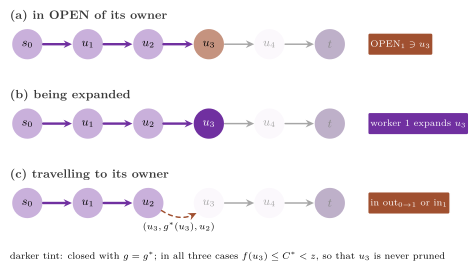
Our next invariant is the parallel form of the one that makes A\(^*\) optimal, i.e., that some node of an optimal path is always in OPEN with its optimal \(g\) (Lemma 2.7); here the node may also be in the hands of a worker or in a message, as Figure 9.3 shows.
Lemma 9.3 (A node of an optimal path is always at hand). Let \(P = (s_0 = u_0, u_1, \ldots, u_k)\) be an optimal path to a goal. While \(z > C^*\), some \(u_j\) of \(P\) with \(g(u_j) = g^*(u_j)\) is (a) in the OPEN list of a worker that stores it, in an entry that is not stale, or (b) being expanded, or (c) in a message (in an outbox, in transit, or drained and not yet inserted) that carries \(g' = g^*(u_j)\).
Proof. We take \(P\) simple (a cycle of an optimal path has cost 0 and
can be removed). Note first that each \(u_j\) has
\(f(u_j) = g^*(u_j) + h(u_j) \le C^* < z\), by admissibility; hence, no
copy of it with its optimal \(g\) is ever pruned at line 12 or at line 20.
At the start, \(s_0\) is in case (a), or about to be inserted by its owner
(line 2). Afterwards, let \(j\) be the largest index such that some node
of \(u_j\) has been closed with \(g(u_j) = g^*(u_j)\) (if there is none,
\(s_0\) has not been expanded yet and is in case (a) or (b)). If the
expansion of \(u_j\) with that \(g\) is still in progress, \(u_j\) is in case
(b). Otherwise, since \(u_j\) is not the goal (otherwise line 9 would have
set \(z \le C^*\)), its expansion generated \(u_{j+1}\) with
\(g' = g^*(u_j) + c(u_j, u_{j+1}) = g^*(u_{j+1})\) (line 11), and this
copy was either given to INSERT at line 13 or sent at line 14. (In an
OperatorDomain the expansion skips the successor that the inverse of
the operator of \(u_j\) leads to, i.e., the parent \(w\) of \(u_j\). If
\(w = u_{j+1}\), then, since the inverse move has the same cost,
\(g^*(u_j) = g(u_j) \ge g(w) + c(w, u_j) \ge g^*(u_{j+1}) + c(u_j,
u_{j+1}) = g^*(u_j) + 2 \, c(u_j, u_{j+1})\) by
Lemma 9.2(ii), i.e., \(c(u_j, u_{j+1}) = 0\) and \(w\) was
expanded with \(g(w) = g^*(u_{j+1})\) when it generated \(u_j\), which
contradicts the choice of \(j\); hence \(u_{j+1}\) is generated.) In the
first case, INSERT either stored \(u_{j+1}\) with \(g^*(u_{j+1})\) and
pushed it, or found \(g(u_{j+1}) \le g'\), i.e.,
\(g(u_{j+1}) = g^*(u_{j+1})\) already; in both cases that node of
\(u_{j+1}\) is open with its optimal \(g\), or being expanded, or closed
with its optimal \(g\), and the last contradicts the choice of \(j\). In
the second case the copy is in a message, case (c), until the worker
that receives it inserts it, after which the argument of the first case
applies. \(\square\)
The end of the search is detected by the mailbox (§9.3). For the moment we take its correctness as a hypothesis, i.e., we assume that the workers stop only when no worker has a node of \(f < z\) in its OPEN list, no worker is expanding a node and no message exists (the condition of Theorem 8.6, with the entries in flight of Definition 8.5), and that they do stop once these hold; Proposition 9.8 proves it on a shared memory, for workers that are each scheduled infinitely often, and Theorem 9.18 over MPI.
Theorem 9.4 (Optimality of HDA\(^*\)). Let the graph be finite, the costs nonnegative and the heuristic admissible, let the node limit be unset and let the detection of the end be correct. Then HDA\(^*\) terminates, with any distribution; if a goal is reachable, it returns a path of cost \(C^*\), and otherwise it reports that there is none.
Proof. Termination. Each insertion of a state with a given \(g\) is followed by at most one expansion of it with that \(g\), and the \(g\) of a node only decreases (Lemma 9.2(ii)); a state has at most \(p\) nodes. Note that each value of \(g\) is the cost of a walk from \(s_0\) that is not larger than the first value assigned. On a finite graph with nonnegative costs these costs form a finite set, since a walk of cost at most \(B\) has at most \(B / \varepsilon\) edges of positive cost, \(\varepsilon\) being the least positive cost, and its cost is a sum of at most that many positive costs taken from a finite set. Hence the expansions are finitely many, and so are the messages, each of which is generated by an expansion; after the last of them is processed no worker has work and no message is in transit, and the detection of the end stops the workers.
Optimality. At the end the conditions above hold; if a goal is reachable and \(z > C^*\), Lemma 9.3 gives a node with \(f \le C^* < z\) in an OPEN list, being expanded or in a message, which contradicts them. Hence \(z \le C^*\), and \(z \ge C^*\) since \(z\) is the cost of a path (Lemma 9.2(iv)). Note that the recorded goal \(t\) still has \(g(t) = C^*\) at the end, since a later decrease of \(g(t)\) would have pushed \(t\) with \(f < z\) and recorded it again at its expansion. The chain of its parents is a path of cost at most \(g(t)\) (Lemma 9.2(iv)), i.e., an optimal one. If no goal is reachable, \(z\) stays \(\infty\), and the search reports the instance unsolvable. \(\square\)
We now bound the scope of the theorem by two remarks. First, on an
infinite (locally finite) graph with costs bounded below by some
\(\varepsilon > 0\) the argument of termination needs a reachable goal
and also that each worker makes progress. Indeed, a worker that is
never scheduled (in practice, one scheduled rarely, e.g., with more
workers than cores, delays the incumbent in the same way) may hold the
only node of an optimal path while the others expand nodes above the
optimum that no incumbent prunes yet (on a finite graph the same
situation costs time and memory rather than termination, and the tester
runs the 15-puzzle with at most one worker per core for this reason, cf.
test_hda in test/test.cpp).
Second, the theorem does not need a consistent heuristic, since the
reopenings are allowed; with a consistent one the sequential A\(^*\) never
reopens (Theorem 2.13), while HDA\(^*\) still
may, and its search overhead counts the reopenings. When the option
node_limit of the sequential search
(Chapter 2) is set, a worker that stores at
least that many nodes after one of its expansions stops the mailbox
(the test is made after each expansion only, so that the insertions
since the previous test may overshoot the limit), all the workers
return, and the status is node_limit, with no claim on the cost.
We end the section with the cost of the steps of the search.
Proposition 9.5 (The cost of a step and the memory of HDA\(^*\)). An expansion of \(u\) that generates the successors \(S\) makes, for each successor not pruned, either one lookup in the closed list of the worker (and at most one insertion in its OPEN list) or one append to an outbox; it takes no lock but the mutex of the goal, when \(u\) is a goal, besides the operations of the channels of the executor, and it computes the owners in the time of Corollary 9.16 when the distribution is incremental. Each batch costs one atomic addition on the shared counter of the mailbox at the sender (two if the queue refuses part of it), and at most one at the receiver, which subtracts all the messages of a drain at once (plus one addition when the drain ends a passive period). With a deterministic distribution the nodes stored by all the workers are at most one per state reached; with any distribution they are at most \(p\) per state.
Proof. The counts are read on Algorithms 9.2 and 9.3: INSERT makes one lookup and at most one push, SEND appends and pushes a full outbox as one batch (one addition, and one subtraction for the part that the channel refuses, cf. line 7 of Algorithm 9.3), and POLL subtracts the messages drained in one addition (with one more addition when the worker leaves the passive state). The bounds on the nodes are those of Lemma 9.1 and of the remark after it. \(\square\)
9.3 The messages and the end of the search¶
Batches and flushes¶
Sending a node usually costs a push on a queue that another worker reads
(on a shared memory) or a message of MPI (e.g., over a network); in both
cases a rather large fixed part of the cost does not depend on the size
of what is sent, and the nodes for the same worker are therefore (rather
naturally) packed into one message, an idea that HDA\(^*\) takes from the
transposition-table-driven scheduling of Romein et al. (cf. section 3 of
[2]). In the library, each worker has one
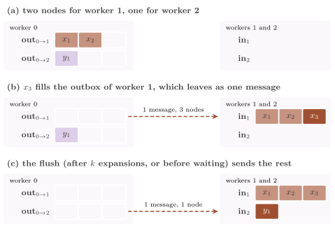
outbox per other worker; a node is appended to the outbox of its owner,
an outbox that holds batch nodes leaves at once as one message, and
the outboxes that are not full leave after each block of flush_period
expansions and before the worker waits (Figure 9.4). We
remark that the flush also matters for the search overhead: a node of an
optimal path that waits in an outbox for others to fill it is a node
that its owner cannot expand, while the owner expands worse nodes and
sends their successors around. Kishimoto et al. observed that packing
"too many" nodes in a message raises the expansions, while packing "few"
raises the cost of the communication (section 5.2 of
[2]); hence, batch and flush_period
trade one overhead for the other.
The channels between the workers are, on every executor, a mesh of bounded queues with one producer and one consumer, one for each ordered pair of workers, and the queue of a pair may be full. The part of a batch that does not fit then stays in the outbox, and it is tried again when a further batch for that worker is ready or at the next flush. A worker whose flush has left something behind keeps polling its inbox (which empties the queues that the others are waiting on); thus, no worker waits for another.
The mailbox and its counter¶
A worker that finds no node of \(f < z\) in its OPEN list cannot stop,
since a node may be travelling to it, or another worker may still
generate one. In fact, the mailbox detects the end by counting, with the
deficit counting of Dijkstra and Scholten [35]
on a single counter \(C\) in the shared memory instead of an
acknowledgment of each message. A worker is active from the start
until a call of QUIESCENT finds its outboxes empty, and it is passive
from then until it drains a message. Each worker \(i\) has an outbox
\(O_j\) for each worker \(j\), with a threshold \(N_j\), at first batch.
Algorithm 9.3 (The mailbox of the workers, on a shared memory).
 1  procedure SEND(i, j, x)                    ▷ i is active
 2     append x to O_j;  if |O_j| ≥ N_j then PUSH(i, j)
 3  procedure PUSH(i, j)                       ▷ nothing once stopped
 4     k ← |O_j|;  C ← C + k                   ▷ before they can be drained
 5     r ← the number of the first messages of O_j that the queue takes
 6     remove them from O_j;  N_j ← |O_j| + batch
 7     C ← C − (k − r)
 8  function FLUSH(i)
 9     for each j with O_j ≠ ∅ do PUSH(i, j)
10     return all the outboxes of i are empty
11  function POLL(i)                           ▷ nothing once stopped
12     M ← ∅
13     for each message x taken from the queues to i do
14        if i is passive then C ← C + 1;  i is active
15        M ← M ∪ {x}
16     C ← C − |M|;  return M
17  function QUIESCENT(i)                      ▷ i has no node of f < z
18     if the mailbox is stopped then return true
19     if i is active then
20        if not FLUSH(i) then return false
21        i is passive;  C ← C − 1
22     return C = 0
23  procedure STOP()                           ▷ from any worker
24     the mailbox is stopped
Definition 9.6 (The deficit counter). The counter \(C\) of Algorithm 9.3 starts at \(p\) (all the workers are active). A worker adds \(k\) to \(C\) before it pushes \(k\) messages and subtracts those that the queue refuses (lines 4 and 7); a passive worker that drains messages adds 1 (it becomes active) before it takes the first of them (line 14), and it subtracts the messages it has drained (line 16). A worker that becomes passive subtracts 1 (line 21), and a passive worker only reads \(C\).
Lemma 9.7 (The counter of the mailbox). Let each worker send only while active and become active only by draining a message. Then (i) at any time \(C\) equals the number of the active workers plus the number of the messages that have been counted by their sender and are still to be subtracted (by their receiver, or by their sender if the queue refuses them), i.e., those in the queues and those being pushed or drained; (ii) the messages in an outbox belong to an active worker; (iii) \(C = 0\) holds only when no worker is active and no message exists, and then it holds forever; (iv) if at some time no worker is active and no message exists, then \(C = 0\) from then on, and every worker that calls QUIESCENT returns.
Proof. (i) By induction on the operations of Algorithm 9.3: each changes \(C\) by the change of the quantity on the right, since a message is counted before it is pushed (hence before it can be drained), uncounted if the queue refuses it, and subtracted after it is drained, and the activity of a worker is added when it leaves the passive state and subtracted when it enters it. (ii) A worker becomes passive only at line 21, after FLUSH has found its outboxes empty, and a passive worker does not send. (iii) Both terms of (i) are nonnegative, so \(C = 0\) forces both to be 0, and by (ii) the outboxes are empty too. From such a state no operation raises \(C\): an addition for a push needs an active sender, and an addition for an activity needs a message to drain. (iv) If no worker is active and no message exists, (i) gives \(C = 0\), and by (iii) it stays 0; each passive worker reads it at its next call of QUIESCENT, at line 22. \(\square\)
The drained messages of line 16 are subtracted before the worker inserts them (lines 5 to 8 of Algorithm 9.2); they are then held by an active worker, and the worker becomes passive only after their insertions and after its next selection has failed. These hypotheses hold for HDA\(^*\), which we now prove together with the progress of the workers on bounded queues.
Proposition 9.8 (The end of HDA\(^*\) on a shared memory). In Algorithm 9.2, without the node limit, (i) a worker returns only when no worker has a node of \(f < z\), none is expanding and no message exists; (ii) if each worker is scheduled infinitely often, every message is eventually pushed and drained, and once the condition of (i) holds every worker returns. With the node limit, all the workers return after the first call of STOP.
Proof. A worker sends only at line 35 of Algorithm 9.2 and in FLUSH,
both while it has work, hence while active. A passive worker has no node
of \(f < z\), since NEXT found none before QUIESCENT, and since \(z\) never
increases (Lemma 9.2(i)) no node of its OPEN list becomes
selectable again: only a message can give it work, and draining one
makes it active. Thus Lemma 9.7 applies. (i) A worker returns at line 14
when QUIESCENT reads \(C = 0\); by Lemma 9.7(iii) no worker is active,
hence none has a node of \(f < z\) or is expanding, and no message exists.
(ii) A message left in an outbox by a full queue is tried again at the
next FLUSH of its sender, which happens every flush_period expansions
and at each call of QUIESCENT while the sender is active; the queue of
the pair empties when its receiver polls, which it does at each
iteration of its loop. Hence no message stays forever in an outbox or
in a queue. Once the condition of (i) holds, Lemma 9.7(iv) makes every
worker return. After STOP the loop of line 4 ends at its next test, and
QUIESCENT returns true. \(\square\)
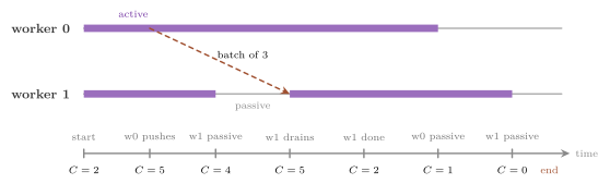
Hence the end that Theorem 9.4 assumes is detected correctly: the workers stop when, and only when, no worker has a node of \(f < z\), none is expanding and no node is in transit; Figure 9.5 follows \(C\) on a run of two workers.
Counting cannot be dropped. A scheme sometimes used in "simple" implementations is made of two rounds of idle flags without any count of the messages: a worker sets its first flag when it has no work, sets its second flag when it sees all the first flags set, and stops when it sees all the second flags set. This scheme is not sound, since a flag carries no information on a message that was pushed after its owner looked at its inbox.
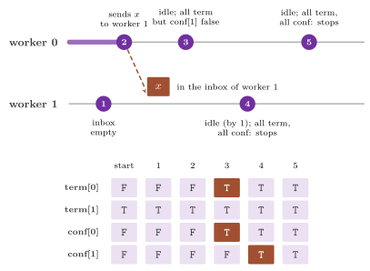
Proposition 9.9 (Idle flags are not enough). With two rounds of idle flags and no count of the messages, two workers may both stop while a node is in the inbox of one of them.
Proof. Figure 9.6 gives such a run. Worker 1 has set its first flag in an earlier round, while it had no work, and it looks at its inbox and finds it empty (event 1). Worker 0 then expands its last node and sends its successor \(x\) to worker 1 (event 2); having no work left, it sets its first flag, sees all the first flags set (that of worker 1 is still set), sets its second flag, and goes on, since the second flag of worker 1 is not set (event 3). Worker 1, acting on what it saw at event 1, has no work: it sees all the first flags and then all the second flags set, and stops (event 4); worker 0, at its next round, sees the same and stops (event 5). Thus, the node \(x\) is never processed; if it is the only node of an optimal path at hand in the sense of Lemma 9.3, the search returns a suboptimal cost, or reports an unsolvable instance. \(\square\)
Nor does it help to let each worker look at its inbox again before it stops: a worker that finds a message there becomes active and may send a node to a worker that has already stopped, which only counting the messages in flight detects.
9.4 The work distributions¶
Much of the behavior of HDA\(^*\) is decided by its distribution, which
balances two overheads against each other: a distribution that keeps the
successors of a node on the worker of the node lowers the communication,
but it tends to gather the nodes of least \(f\) on a few workers, while
one that spreads the states uniformly balances the load at the price of
sending almost all the nodes. The band effect of Jinnai and Fukunaga
(section 3.1.1 of [5]) explains the (somewhat
indirect) link between the load balance and the search overhead: if,
with two workers, a worker owns a fraction \(q\) of the nodes of each
value of \(f\), its \(n\)-th expansion is roughly the \((n / q)\)-th of A\(^*\),
and the farther \(q\) is from \(1 / 2\) the more the workers expand out of
the order of A\(^*\), i.e., nodes that A\(^*\) would not reach (an
estimate of [5], not a theorem). We now
describe the six distributions of Distribution.h that
take their structure from the Domain, and then the Zobrist hashing on a
table given by the caller, on which the hand-made projections and the
automatic distributions of Chapter 10
are built, in the notation \(\mathrm{HDA}^*[\mathit{hash},
\mathit{abstraction}]\) of section 2.6 of [5] and
by their names in the library;
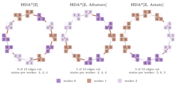
Figure 9.7 colours the 12 states of the \(2 \times 2\) puzzle
by their owner under three of them.
From a hash to a worker¶
A distribution that computes a 64-bit hash \(h\) maps it to a worker by
the multiply-high reduction of Lemire [151],
$\(\mathrm{reduce}(h, p) = \left\lfloor \frac{h \, p}{2^{64}}
\right\rfloor,\)$
which uses the high bits of \(h\). The code computes it by halves in 64-bit
arithmetic, with the same result on every compiler
(Distribution.h:103-104): with \(h = a\,2^{32} + b\)
and \(b < 2^{32}\), \(\lfloor h p / 2^{64} \rfloor = \lfloor (a p + \lfloor b
p / 2^{32} \rfloor) / 2^{32} \rfloor\), where \(a p \le 2^{64} - 2^{33} + 1\)
and \(\lfloor b p / 2^{32} \rfloor < 2^{32}\) for \(p < 2^{32}\), so that no
sum overflows. A 32-bit key \(k\) is mapped by key_owner, i.e., to
\(\mathrm{reduce}(2^{32} k, p) = \lfloor k p / 2^{32} \rfloor\), the key
standing for the high 32 bits of the hash.
Proposition 9.10 (The reduction is balanced).
For \(0 \le i < p \le 2^{64}\), the number of the values \(h \in \{0,
\ldots, 2^{64} - 1\}\) with \(\mathrm{reduce}(h, p) = i\) is either
\(\lfloor 2^{64} / p \rfloor\) or \(\lceil 2^{64} / p \rceil\); the same
holds for key_owner with \(2^{32}\) in place of \(2^{64}\).
Proof. \(\mathrm{reduce}(h, p) = i\) if and only if \(i \le h p / 2^{64} < i + 1\), i.e., \(h \in [\, i \, 2^{64} / p, (i + 1) \, 2^{64} / p)\), a half-open interval of length \(2^{64} / p\), which contains either \(\lfloor 2^{64} / p \rfloor\) or \(\lceil 2^{64} / p \rceil\) integers. \(\square\)
Hence, for a uniform hash, the share of the states of each worker differs from \(1 / p\) by less than \(2^{-64}\) (or \(2^{-32}\) for a key), i.e., the reduction adds (almost) no imbalance; the modulo \(h \bmod p\), which the library uses only where the comparison of [5] requires it (below), has the same property but costs a division.
Zobrist hashing, HDA\(^*\)[Z]¶
With the state \(s\) described by the set \(F(s)\) of the features that hold in it and a table \(R\) of random 64-bit strings, one per feature, the Zobrist hash [152] is
with \(\oplus\) the exclusive or of the bits (equation (1) of
[5]); ZobristDistribution
(Distribution.h:134, for a FeatureDomain) draws \(R\)
from the seed, takes as the key the high 32 bits of \(Z(s)\) and as the owner
that of the key. This is the original distribution of HDA\(^*\) (section 3 of
[2]). The following procedures, in which the
table \(T\) is \(R\) for Zobrist hashing and the table \(R'\) of Abstract
Zobrist hashing laid out by raw feature (see below), are those of both
distributions; xor is the exclusive or of the bits.
Algorithm 9.4 (The Zobrist hash, its key and its owner).
 1  function HASH(s)
 2     y ← 0
 3     for each feature x of s do y ← y xor T[x]
 4     return y
 5  function KEY(s)
 6     return the high 32 bits of HASH(s)
 7  function KEY(k, s, t)               ▷ t a successor of s, k = KEY(s)
 8     for each feature x that holds in exactly one of s and t do
 9        k ← k xor (the high 32 bits of T[x])
10     return k
11  function OWNER(s, p)
12     return floor(KEY(s) · p / 2^32)
Zobrist hashing spreads the states over the workers regardless of the structure of the graph. Its statistical properties are those of the following proposition, in which we take, as the analysis of hashing does, the entries of \(R\) independent and uniform on \(\{0, 1\}^{64}\); the table of the library is drawn by a pseudo-random generator from the seed, to which the statement applies only as a model.
Proposition 9.11 (The independence of Zobrist hashing). Let the entries of \(R\) be independent and uniform. (i) For two distinct nonempty sets of features \(S \ne T\), the pair \((Z(S), Z(T))\) is uniform on \(\{0, 1\}^{128}\), i.e., \(Z\) is pairwise independent on the nonempty sets. (ii) If each state has exactly one feature per position, i.e., the features are the pairs (position, value) and a state gives one value to each position (as the cell of each tile on a sliding-tile puzzle), then \(Z\) is 3-independent, i.e., the hashes of three distinct states are independent and uniform. (iii) On sets of varying size \(Z\) is not 3-independent in general.
Proof. (i) Some feature \(x\) lies in exactly one of the two sets, say in \(S \setminus T\). Given all the entries of \(R\) but \(R[x]\), \(Z(T)\) is fixed and uniform over the choice of those entries (since \(T\) is nonempty and does not contain \(x\)), while \(Z(S)\) is \(R[x]\) xor a fixed string, hence uniform and independent of \(Z(T)\). (ii) Here \(Z\) is the simple tabulation hashing of the tuple of the values. Let \(a\), \(b\) and \(c\) be three distinct states. At a position where they do not all agree, either their three values are distinct or exactly two are equal, and in both cases one of the three states, say \(a\), has a value that the other two do not have; such a position exists, since the states are distinct. Given all the entries but that of \(a\) at this position, \(Z(b)\) and \(Z(c)\) are fixed, and \(Z(a)\) is uniform; hence \(Z(a)\) is uniform and independent of \((Z(b), Z(c))\), which by (i) is uniform on pairs. (iii) With \(S = \{x\}\), \(T = \{y\}\) and \(U = \{x, y\}\) one has \(Z(U) = Z(S) \oplus Z(T)\). \(\square\)
Corollary 9.12 (The communication of Zobrist hashing). Under the hypothesis of Proposition 9.11, for two states \(s\) and \(t\) with distinct nonempty sets of features, the probability that \(\mathrm{owner}(s) = \mathrm{owner}(t)\) lies in \([1/p, 1/p + 2^{-32}]\); hence a successor not pruned is sent to another worker with probability between \(1 - 1/p - 2^{-32}\) and \(1 - 1/p\).
Proof. By Proposition 9.11(i) the keys of \(s\) and \(t\), the high 32
bits of their hashes, are independent and uniform on \(\{0, \ldots,
2^{32} - 1\}\). Let \(n_i\) be the number of keys that key_owner maps to
\(i\); the probability of equal owners is \(\sum_i n_i^2 / 2^{64}\). Since
\(\sum_i n_i = 2^{32}\), the Cauchy-Schwarz inequality gives \(\sum_i n_i^2
\ge 2^{64} / p\), and since \(n_i \le 2^{32} / p + 1\) by Proposition 9.10,
\(\sum_i n_i^2 \le (2^{32} / p + 1) \, 2^{32}\). \(\square\)
The corollary is the reason for \(\mathrm{CO} \approx 1 - 1/p\) under
Zobrist hashing (section 2.4 of [5], where
this is noted for an ideal uniform assignment). It concerns a fixed
pair of states; the fraction measured in a run is an average over the
successors that the search generates, which depend on the owners
themselves, and since the counter generated also counts the pruned
successors, the measured \(\mathrm{CO}\) is typically somewhat below
\(1 - 1/p\). The hash of a successor can be updated from that of its
parent in the time of the features that the move changes
(§9.5).
Abstract Zobrist hashing, HDA\(^*\)[Z, Afeature]¶
Jinnai and Fukunaga combine the hashing with a projection \(A\) of the features onto fewer abstract features (section 4 of [5], equation (2)):
with a table \(R'\) of random strings indexed by the abstract features.
AbstractZobristDistribution (Distribution.h:203, for
an AbstractFeatureDomain) lays its table out by raw feature, i.e., its
constructor draws \(R'\) from the seed and stores \(T[x] = R'[A(x)]\) at the
index of each raw feature \(x\) (Algorithm 3 of
[5]); thus, the hash costs as much as \(Z\)
and is computed and updated by the same procedures of Algorithm 9.4. A
move that changes no abstract feature keeps the successor on the worker
of its parent, which lowers the communication; we make this precise.
Corollary 9.13 (The owners under AZ). If every feature that holds in exactly one of \(s\) and \(t\) has an abstract feature that appears an even number of times among those of the changed features (e.g., a move that changes \((k, c)\) into \((k, b)\) with \(A(k, c) = A(k, b)\)), then \(\mathit{AZ}(t) = \mathit{AZ}(s)\), and \(t\) has the owner of \(s\) for every \(p\).
Proof. By Proposition 9.15 below, \(\mathit{AZ}(t) = \mathit{AZ}(s) \oplus \bigoplus_x R'[A(x)]\) over the changed features \(x\), and the entries of an abstract feature that appears an even number of times cancel, since \(y \oplus y = 0\). \(\square\)
Also, the hashing of all the abstract features keeps the load (rather) balanced: \(\mathit{AZ}(s)\) is the Zobrist hash, with the table \(R'\), of the set of the abstract features that appear an odd number of times in \(s\), and the statement of Corollary 9.12 holds for two states whose such sets are distinct and nonempty; on the domains of section 4.1 of [5], the 15-puzzle and the 24-puzzle among them, AZ was the best of the distributions compared there. On the sliding-tile puzzles one can take as the abstract feature of a tile the half of the board that holds it, as the library does, and then a move changes it only when it slides a tile vertically across the middle line; on the \(2 \times 2\) puzzle of Figure 9.7 (middle) the halves are the rows, a horizontal move always keeps the owner, and at most half of the edges are cut.
We remark that a state in which two raw features have the same abstract feature has the two entries cancelled in \(\mathit{AZ}\), since \(R'[a] \oplus R'[a] = 0\). The hash is still a function of the state (which is all that the correctness of §9.2 requires), but its values are less uniform. On the sliding-tile puzzles this never happens, since each tile is in one cell.
Abstraction, HDA\(^*\)[Z, Astate]¶
AbstractStateDistribution (Distribution.h:413, for an
AbstractStateDomain) sends all the states with the same abstract state
to the same worker, hashing the abstract state with a seeded mix (the
64-bit mixing function SplitMix64 of the abstract state xor the mixed
seed, not a Zobrist hash of its features), and reducing the result by
\(\mathrm{reduce}\). This is AHDA\(^*\) of Burns et al.
[3] with a uniform hash in place of their
perfect hash (hence the notation HDA\(^*\)[Z, Astate] rather than
HDA\(^*\)[P, Astate], cf. section 2.5 of [5]).
Since the owner is a function of the abstract state, a successor changes
worker only when it changes the abstract state, and its communication is
the least of these distributions; but no mechanism balances the load:
the abstract states are usually "few", and those that contain the nodes
of least \(f\) may belong to few workers, which raises the search
overhead. On the 15-puzzle the abstraction is the triple of the cells of
tiles 1, 2 and 3, i.e., \(16 \cdot 15 \cdot 14 = 3360\) abstract states.
Perfect hashing, HDA\(^*\)[P]¶
PerfectHashDistribution (Distribution.h:449, for a
PerfectHashDomain) takes the rank of the state modulo \(p\). This is the
distribution called "HDA\(^*\)" in [3], and
Jinnai and Fukunaga found that on the sliding-tile puzzles it has both a
high search and a high communication overhead (sections 3.2 and 4.1 of
[5]); the library keeps it to reproduce that
comparison. The reason, at least on the puzzles, lies in the following
proposition, which states for the rank of the library what footnote 5 of
section 3.1.4 of [5] observes for \(p = 8\).
Proposition 9.14 (The perfect hash modulo
\(p\)). Let the board have \(n\) cells, let \(\mathrm{pos}(k)\) be the cell of
tile \(k\) (the blank being tile 0), and let the rank be the one of
SlidingTile.h:590-603, i.e.,
$\(\mathrm{rank}(s) = \sum_{k=0}^{n-1} d_k \, (n - 1 - k)!, \qquad d_k =
|\{\, j > k : \mathrm{pos}(j) < \mathrm{pos}(k) \,\}|.\)$
If \(m\) is the least integer with \(p \mid m!\), then \(\mathrm{rank}(s)
\bmod p\) depends only on the relative order of the cells of the tiles
\(n - m, \ldots, n - 1\).
Proof. The code computes \(\mathrm{rank} \gets \mathrm{rank} \cdot (n - k) + d_k\) for \(k = 0, \ldots, n - 1\), which expands to the sum above. Also, \(d_k\) is the cell of tile \(k\) minus the number of the cells below it that the tiles \(0, \ldots, k - 1\) occupy, i.e., the number of the tiles \(j > k\) below it. For \(k < n - m\) one has \(n - 1 - k \ge m\), hence \(p\) divides \((n - 1 - k)!\) and the term vanishes modulo \(p\); the remaining \(d_k\), \(k \ge n - m\), compare the cells of the tiles \(n - m, \ldots, n - 1\) only. \(\square\)
On the 15-puzzle with \(p = 8\) one has \(m = 4\), and the owner depends on the relative order of the cells of the tiles 12, 13, 14 and 15 alone: a move that changes this order may change the owner, any other move keeps it, and the classes of states that share an owner follow neither the load nor the locality of the search. We remark that over all the boards the residues are (almost) equally frequent, the rank being a bijection onto \(\{0, \ldots, n! - 1\}\); what the proposition rules out is a balance of the nodes that the search reaches at each value of \(f\), which nothing in the distribution controls.
The hash of the closed list, and a random owner¶
StateHashDistribution (Distribution.h:477, the
default of both searches) remixes the hash that any Domain gives to its
closed list with a seed, by the same mix as above; it behaves as Zobrist
hashing for any Domain to the extent that the hash of the Domain is
uniform, with no feature to define, but it cannot be updated by a move.
RandomDistribution (Distribution.h:598) sends each
generated state to a worker drawn at random, as in the randomized strategies of
Kumar, Ramesh and Rao and of Karp and Zhang (cf. section 6 of
[2]). Hence, a state has no owner, a
duplicate is detected only when its copies happen to reach the same
worker, and each worker needs a separate generator (which the class
declares by per_worker; HDA\(^*\) gives each worker a copy of the
distribution, all of them seeded alike). It is the baseline without
detection of the duplicates across the workers; Kishimoto et al. report
that on their planning benchmarks, with 16 cores and 2 GB per core, it
ran out of memory on every instance, and that with 32 GB per core it
expanded more than an order of magnitude more nodes than HDA\(^*\)
(section 6 and Table 8 of [2]).
Zobrist hashing on a given table¶
TableZobristDistribution (Distribution.h:335, for
a FeatureDomain) is Zobrist hashing on a table \(R\) that the caller gives,
one entry per feature (a missing entry being 0), together with a name that
says how the table was built; its hash, its key and its owner are computed
and updated by the procedures of Algorithm 9.4 with \(T = R\), so that
Proposition 9.15 and Corollary 9.16 hold for it,
and it is an IncrementalDistribution when the Domain is an
IncrementalFeatureDomain. The table may be that of a projection written
out as a FeatureAbstraction (Distribution.h:274),
i.e., the vector of the abstract feature of each feature (or
no_abstract_feature, Domain.h:334, for a feature that
the projection ignores) and the number of the abstract features; its
table( seed ) holds \(R'[A(x)]\) at each feature \(x\), with \(R'\) drawn from
the seed, and 0 at the ignored ones, of() builds it from a vector, and
identity( n ) is the projection of Zobrist hashing. With the same seed,
the table of the identity is that of ZobristDistribution, and the table
of the projection of an AbstractFeatureDomain that of
AbstractZobristDistribution, since the random words of a table are drawn
one after the other from the seed
(Proposition 10.1); the three classes
then give every state the same owner. The table distribution is therefore
Abstract Zobrist hashing with any projection, not only the one that the
Domain provides: an ignored feature has the entry 0 and changes no key,
so that ignoring all the features but those of a few tiles hashes the
abstract state of AHDA\(^*\) by Zobrist hashing (HDA\(^*\)[Z, Astate]) instead
of the mix of AbstractStateDistribution. The projections of the
sliding-tile puzzles compared by Jinnai and Fukunaga (by rows, pairs of
cells, blocks of \(2 \times 2\) cells, halves of the board, and the regions
of the 24-puzzle) are given by SlidingTile::tile_abstraction(), and the
projections and the tables built from a sample of the instance by
AutoDistribution.h; both are described in
Chapter 10. Unlike the other classes,
whose name is a static method, its name() is the member given at the
construction.
The hyperplanes of a levelled graph¶
HyperplaneDistribution (Distribution.h:531, for
a LevelDomain, Domain.h:396) is the hyperplane work
distribution HDA\(^*\)[Hyperplane] of Kobayashi, Kishimoto and Watanabe
[43], which assigns to the workers, modulo \(p\),
the planes of consecutive levels of a levelled graph (e.g., the total
length of the prefixes aligned in the multiple sequence alignment), so
that the states reached by several paths meet on fewer workers. Its
owner is a function of the level and of the hash of the state, it is not
incremental, and it is described, with its thickness and the alignment
on which it is used, in Chapter 15.
A summary¶
The following table gathers what each distribution needs and what it trades; the overheads are those that the scheme leads one to expect, and only measurements (cf. §9.8) decide among them on a given domain.
| Name | Needs | Incr. | Det. | CO | Load |
|---|---|---|---|---|---|
| Z | FeatureDomain |
yes | yes | about \(1 - 1/p\) | balanced |
| AZ | AbstractFeatureDomain |
yes | yes | below Z | balanced |
| A | AbstractStateDomain |
no | yes | lowest | not controlled |
| P | PerfectHashDomain |
no | yes | high | not controlled |
| H | Domain |
no | yes | about \(1 - 1/p\) | balanced |
| R | Domain |
no | no | about \(1 - 1/p\) | balanced |
| T | FeatureDomain and a table |
yes | yes | that of the table | that of the table |
| Hyperplane | LevelDomain |
no | yes | low on a levelled graph | by planes |
The column "Incr." gives whether the distribution is an
IncrementalDistribution (Z, AZ and T when the Domain is an
IncrementalFeatureDomain), "Det." whether the owner is a function of
the state, and the load of AZ is balanced only if the abstract features
are many with respect to \(p\); the overheads of T are those of the
projection or of the construction of its table, and those of the
hyperplanes are discussed in Chapter 15. The
first six distributions are made "by hand", the features, the projection
or the abstraction coming from the Domain. The choice of the table of T
from the problem (by partitioning the transition graphs of the features,
by the operators, by a state abstraction, or by a subspace of the kernel
of the key, each estimated on a sample) is the subject of
Chapter 10.
9.5 Incremental Zobrist hashing¶
A hash computed from scratch reads all the features of the state, i.e.,
\(n - 1\) entries of the table on a puzzle of \(n\) cells; Zobrist hashing
can instead be updated by a move, from the hash of the parent and the
features that the move changes (section 3 of
[2] and section 2.4 of
[5]). We now state the identity on which the
update (lines 7 to 10 of Algorithm 9.4) rests, for the sets of features
\(F(s)\) and \(F(t)\) of a state and of its successor, whose symmetric
difference \(F(s) \triangle F(t)\) is enumerated by
for_each_feature_change().
Proposition 9.15 (Incremental Zobrist hash). For any two states \(s\) and \(t\),
and the same holds for \(\mathit{AZ}\) with the table laid out by raw feature, and for the keys, i.e., for the high 32 bits of \(Z\) and of \(\mathit{AZ}\).
Proof. The set \(\{0, 1\}^{64}\) with \(\oplus\) is an abelian group in
which each element is its own inverse. Hence
$\(Z(s) \oplus Z(t) = \bigoplus_{x \in F(s)} R[x] \oplus \bigoplus_{x
\in F(t)} R[x] = \bigoplus_{x \in F(s) \triangle F(t)} R[x],\)$
since each feature of \(F(s) \cap F(t)\) appears twice and cancels, and
\(\oplus\) with \(Z(s)\) on both sides gives the claim. For \(\mathit{AZ}\)
the same computation holds with the entry \(R'[A(x)]\) stored at the
index of \(x\), which is how AbstractZobristDistribution computes both
the hash and its update. Finally, taking the high 32 bits, i.e., \(y
\mapsto \lfloor y / 2^{32} \rfloor\), commutes with \(\oplus\), since the
exclusive or acts bit by bit; hence the identity holds for the keys as
well. \(\square\)
Corollary 9.16 (Owners from the parent). For a
distribution that is an IncrementalDistribution, the function that
successor_owners() returns maps each successor \(t\) of a node of state
\(s\) and key \(k\) to ( owner( t , p ) , key( t ) ), and it costs
\(|F(s) \triangle F(t)|\) lookups in the table instead of the \(|F(t)|\) of
a computation from scratch.
Proof. key( k , s , t ) applies the identity of
Proposition 9.15 to the key \(k\) of \(s\) (lines 7 to 10 of
Algorithm 9.4), with one lookup per changed feature, and the owner is
key_owner() of the key, as for owner( t , p ). \(\square\)
Our tester checks the corollary on random walks of the 8-, 15- and
24-puzzles, for \(p \in \{1, 2, 3, 7, 64\}\), against the owners and the
keys computed from scratch (check_successor_owners in
test/test.cpp).
On the sliding-tile puzzles a move slides one tile \(k\) from a cell \(c\)
to the cell \(b\) of the blank, and the symmetric difference is \(\{(k, c),
(k, b)\}\): two entries of the table instead of 15 on the 15-puzzle (and
none for the state being expanded, whose key is stored in its node).
Both cells are found without locating the blanks: the packed states
\(s\) and \(t\) differ only in the fields of the cells \(b\) and \(c\), both
of which hold \(k\) in \(s \oplus t\), and therefore two counts of trailing
zeros of \(s \oplus t\) give them
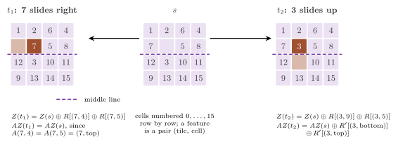
(SlidingTile.h:420-431). Figure 9.8
shows the update for a move inside a half of the board and for one across the
middle line.
9.6 HDA\(^*\) over MPI¶
HDAStarMPI (HDAStarMPI.h) is the search of §9.2
with one MPI process per worker, as in the original implementation of Kishimoto
et al., where the workers are MPI processes even on a single multicore
machine (section 3 of [2]). Since the
processes share no memory, a node records the state of its parent
rather than a pointer, the incumbent travels as a message to all the
other processes, and the state and the cost types must be trivially
copyable, since the nodes travel as bytes (a static assertion checks the
state type, HDAStarMPI.h:114). MPI is
initialized by the caller (with at least MPI_THREAD_FUNNELED if the
Domain uses threads), all the processes of the communicator call
solve(), and all of them return the same Solution.
Algorithm 9.5 (HDA\(^*\) over MPI, on the process \(i\)).
 1  procedure HDA*-MPI(s₀) on the process i
 2     z ← ∞;  if owner(s₀) = i then INSERT(s₀, 0, nil)
 3     loop
 4        for each message m received do
 5           if m is a batch of nodes then INSERT each of them
 6           else if m is an incumbent z' then z ← min(z, z')
 7           else if m is a stop then stop expanding
 8        if OPEN_i has a node of f < z then
 9           expand it as at lines 7 to 15 of HDA*, a goal that lowers z
               sending z to all the other processes
10        else send all the outboxes
11        if OPEN_i has no node of f < z and the mailbox detects the end
12           then break
13     the process of the least goal broadcasts it, and the path is rebuilt
         from it, each state broadcast with its parent by its owner
14     the sends in progress complete
This is the pseudocode of HDAStarMPI.h:14-31. In the
library, the batches are sent with nonblocking sends (MPI_Isend), whose
buffers are kept until MPI has completed them, and received with MPI_Iprobe
and MPI_Recv from any process; the mailbox duplicates the
communicator, and its messages never meet those of the program. The
messages are a variant of a node and an incumbent, and the reception and
the rebuilding of the path are made as follows, the parent of a node
being a state, nil at the root.
Algorithm 9.6 (The reception and the path over MPI).
 1  procedure RECEIVE()                         ▷ on the process i
 2     M ← ∅
 3     for each message m drained from the mailbox do
 4        if m is a node then M ← M ∪ {m}
 5        else z ← min(z, the cost of the incumbent m)
 6     for each (v, g', u) ∈ M do               ▷ phase 1
 7        compute the hash of v;  prefetch its place in CLOSED_i
 8     for each (v, g', u) ∈ M do INSERT(v, g', u)        ▷ phase 2
 9  procedure PATH()                            ▷ on every process
10     if some process hit the node limit then return node_limit
11     (c, r) ← the least cost of a recorded goal and its process
12     if c = ∞ then return unsolvable
13     (s, γ, u) ← the goal of r, its g and its parent, broadcast by r
14     π ← (s)
15     while u ≠ nil do
16        j ← owner(u)
17        (s, γ', u) ← u, the parent of its node at j, broadcast by j
18        π ← (s) followed by π
19     return the path π, of cost γ
Line 10 is a reduction (the maximum of the flags of the processes), and
line 11 a reduction with MPI_MINLOC (HDAStarMPI.h:383),
after the counters of all the processes have been gathered (MPI_Allgather).
Over MPI the counter messages is the number of the batches sent,
those that carry only incumbents included, while sent counts nodes
only; hence, unlike on a shared memory, messages may exceed sent.
We let each process keep an incumbent \(z_i\), the least cost that it has found or received; since \(z_i\) is never smaller than the least cost \(z\) found by any process, a process prunes less than a shared \(z\) would, which may cost expansions (how many depends on the latency of the incumbent messages) but not correctness.
The termination detection of Mattern¶
Over MPI, the end is detected by the four counters of Mattern [11], in the form described in section 3 of [2] and in section 3.3.1 of [1]. Kishimoto et al. used the time algorithm of Mattern, a variation that needs one wave only, while the library uses the basic method with two waves. Each process \(i\) counts the messages that it has sent, \(s_i\), and those that it has received, \(r_i\), both nondecreasing. We say that a process is passive when it has no node of \(f < z_i\) and has posted all its outboxes, and it becomes active only by receiving a message (an incumbent never gives work, and a node usually may). Note that a process with work never contributes to a wave.
Definition 9.17 (Waves). A wave is a
nonblocking reduction (MPI_Iallreduce) of the pairs \((s_i, r_i)\) of
all the processes into their sums \((S, R)\); a process contributes to a
wave only when it is passive, i.e., from QUIESCENT, at an instant
\(t_i\), and it keeps receiving and working while the wave completes. A
process starts the wave \(k\) only after the wave \(k - 1\) has completed
for it. The end is declared at the first wave \(k \ge 2\) whose sum of the
sends \(S_k\) equals the sum of the receipts \(R_{k-1}\) of the wave before.
Algorithm 9.7 (QUIESCENT over MPI, on the process \(i\) of \(p\), with no node of \(f < z_i\)). The wave also sums a flag stopped of each process, \(X\) is the number of the processes stopped, \(k\) counts the waves completed, and \(R'\) is the sum of the receipts of the last wave.
 1  function QUIESCENT()
 2     if the end is known then return true
 3     post all the outboxes, by nonblocking sends
 4     if a wave is in progress then
 5        if it has not completed then return false
 6        k ← k + 1;  (S, R, X) ← its sums
 7        if X = p then the end is known;  return true   ▷ all stopped
 8        if k > 1 and S = R' then the end is known;  return true
 9        R' ← R
10     start a wave, the nonblocking sum of (s_i, r_i, stopped)
11     return false
Since a reduction completes for a process only after all the processes have contributed to it, each contribution to the wave \(k\) comes after all the contributions to the wave \(k - 1\): if \(t_i^{k}\) is the instant of the contribution of \(i\) to the wave \(k\), then \(t_j^{k} > \max_i t_i^{k-1}\) for all \(j\). A single wave is not enough, as the left half of Figure 9.9 shows. In fact, the counters of a wave are read at different instants. A message sent before the cut and received after it is counted by \(S\) but not by \(R\), while one sent after the cut and received before it is counted by \(R\) only. The two errors may cancel while a message is in flight.
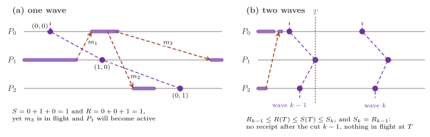
Theorem 9.18 (Mattern's four counters detect the end exactly). Let each process send only while active and become active only by receiving, and let \(T = \max_i t_i^{k-1}\). (i) If \(S_k = R_{k-1}\), then at the instant \(T\) all the processes were passive and no message was in transit; hence the computation had ended at \(T\), and the end is never declared before it happens. (ii) If the computation ends at some instant \(T^*\) and each process keeps calling QUIESCENT, then the end is declared, at the latest at the second wave all of whose contributions follow \(T^*\), and all the processes declare it at the same wave.
Proof. (i) Let \(S(t) = \sum_i s_i(t)\) and \(R(t) = \sum_i r_i(t)\). A message is received only after it is sent; hence, \(R(t) \le S(t)\) at all times, and the counters are nondecreasing. Since \(t_i^{k-1} \le T\) for all \(i\), one has \(R_{k-1} = \sum_i r_i(t_i^{k-1}) \le R(T)\), and since \(t_i^{k} > T\) for all \(i\), one has \(S(T) \le \sum_i s_i(t_i^{k}) = S_k\). Therefore
and all are equalities. From \(R(T) = R_{k-1}\) and the monotonicity of each \(r_i\) it follows that \(r_i(T) = r_i(t_i^{k-1})\) for each \(i\), i.e., no process received a message between its contribution to the wave \(k - 1\) and \(T\). Since it was passive at its contribution and it can become active only by receiving, it was passive at \(T\). From \(S(T) = R(T)\), no message was in transit at \(T\). A computation in which all the processes are passive and no message is in transit has ended, and it stays so, since nobody can send.
(ii) After \(T^*\) no message is sent or received; thus, \(S\) and \(R\) are constant and equal, say to \(N\). Every process is passive and calls QUIESCENT, and therefore each wave completes in finite time; let \(W\) be the first wave all of whose contributions follow \(T^*\) (it exists, since the contributions to a wave follow those to the wave before). Then \(R_W = N\) and \(S_{W+1} = N\), and the end is declared at the wave \(W + 1\) at the latest. The sums of a reduction are the same on all the processes, and so is the decision. \(\square\)
The end that Theorem 9.18 detects is the end assumed by Theorem 9.4. At that instant all the incumbents sent have been received; hence, each \(z_i\) equals the least cost found by any process; no process has a node of \(f < z\), none is expanding, and no node is in transit. Hence, the proof of Theorem 9.4 applies word for word, with \(z_i\) in the pruning of the process \(i\) (which, as remarked above, prunes no more than \(z\) would). A wave runs while the processes keep working, and a process never waits for one; its latency is that of a reduction of MPI, typically logarithmic in the number of processes, which depends on the implementation of MPI and which we do not prove.
A process that reaches the node limit sends a note (an empty batch) to
each other process; a process that sees it stops expanding and
contributes to the waves as stopped, and the computation ends at the
first wave to which all have contributed stopped (line 7 of Algorithm
9.7). The notes are not counted by the waves, which a stop ends by the
flags alone. When the mailbox is destroyed, at the end of solve() and
after the path has been rebuilt, the messages still in flight (which
exist only after a stop) are received and dropped, through a collective
exchange of the number of the messages that each process has sent to
each other one (MPI_Reduce_scatter_block), and the pending sends are
completed.
The path¶
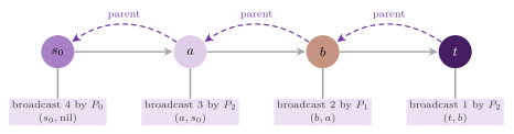
We rebuild the path after the end, by the procedure PATH of Algorithm
9.6 (Figure 9.10): each process knows the next parent,
hence its owner, and the owner looks it up in its closed list. This is
why the distribution of HDAStarMPI must be deterministic: with the
random owner, the process queried for a state need not be the one that
stores it. We now prove that the rebuilding is sound.
Lemma 9.19 (The path over MPI). With a deterministic distribution and without the node limit, at the end of HDA\(^*\) over MPI: (i) each state reached has one node, at its owner; (ii) the parent of each stored node other than the root is a state that has a node at its owner, so that the lookup of line 17 of Algorithm 9.6 never fails; and (iii) the chain of the parents of the goal is a path from \(s_0\) of cost at most its \(g\), which PATH rebuilds with one broadcast per state.
Proof. (i) is Lemma 9.1. (ii) The parent of a node is set from a message \((v, g', u)\), created by the expansion of the node of \(u\) at the owner of \(u\), and nodes are never deleted. (iii) By (i), a parent state names one node, and the proof of Lemma 9.2(ii) to (iv) holds with the parent states in the place of the pointers; hence the chain is acyclic, ends at \(s_0\), whose parent is nil, and has cost at most \(g(t)\). Each iteration of line 15 adds one state with one broadcast, and all the processes run the same iterations, since each broadcast gives them the same values. \(\square\)
9.7 The engineering of the implementation¶
The algorithm of §9.2 leaves much freedom to the implementation, and we use it as follows.
- The inbox is drained as a whole, and the hashes of all its nodes are computed and their slots in the closed list prefetched before the first lookup (lines 5 to 8 of Algorithm 9.2, and lines 6 to 8 of Algorithm 9.6 over MPI). A message from another worker typically carries a state that the receiver has not touched recently, and its lookup is then likely to be a "cold" miss.
- The incumbent is an atomic variable on a separate cache line, and
each worker is aligned to a cache line (
HDAStar.h:250and:260), and the counters and the lists of one worker do not share a line with those of another. Also, the pruning tests read the incumbent with a relaxed load: a stale value is larger than the current one (the incumbent only decreases), and therefore it prunes less, never more. - Each worker allocates its nodes from a private pool and keeps its closed list in a private table (cf. Chapter 3); the memory of a node is therefore written by one thread only, which is the content of Lemma 9.1.
- The key of a node, 32 bits, is stored in the node, where it fits in the padding of a node whose state is one or two words; the key of the state being expanded is never recomputed.
- With integer costs the OPEN list is a list of buckets, as in the sequential search; otherwise it is a binary heap.
- A batch costs one atomic addition at the sender and at most one at the receiver on the counter of Definition 9.6 (Proposition 9.5), and a passive worker only reads that counter.
9.8 Benchmark¶
Table 9.1. HDA\(^*\) with the distributions Z, AZ and P on the threads, and with Z and AZ on OpenMP, on FastFlow and over MPI, on the 15-puzzle.
| search | 1 | 2 | 4 | 8 | 16 | 32 | 48 | 64 | 96 |
|---|---|---|---|---|---|---|---|---|---|
Placeholder: the results of this table are to be measured on an idle machine and written here by manual/build/tables.py; no number is given until then.
The experiment runs on 12 of the 100 instances of Korf
[7] (the instances 1, 3, 10, 14, 15, 22, 26,
27, 32, 33, 37 and 52, as listed in tools/bench/campaign.sh),
with the Manhattan distance, the default batches of 64 nodes and flushes every
64 expansions, on 1, 2, 4, 8, 16, 32, 48, 64 and 96 cores. A row is a
search, i.e., HDA\(^*\) with its distribution in brackets and its runtime
(thread, openmp, fastflow or mpi), or the sequential A\(^*\) with the OPEN
list on buckets, against which the speedups are computed; a column is
the number of cores given to the search (one worker per core, the
workers pinned, and over MPI one process per core). A cell gives the
seconds summed over the instances, each instance counting with the
median of its two runs, and in parentheses the speedup over the
sequential A\(^*\) on 1 core; a cell is empty when the search did not solve
all the instances. The machine, the compiler and the A/A noise (the
gap between the two runs of the same search, which are made in two
processes) are stated in the note under the table. All costs are
integers; each run writes the cost it found in the records of the
campaign, where it can be compared with that of the sequential search
(the table does not show it, and a run counts in a cell as soon as it
reports a solution). We measure the wall-clock time of solve(), i.e., from
the creation of the workers to the solution, the tracing of the path
included; since the benchmark gives no executor to the search, the start
of the threads is included as well (over MPI, the time is that of the
process of rank 0, the duplication of the communicator and the final
gathering of the counters included). The time does not include the
start of the process, the reading of the instance, the construction of
the Domain and of the tables of the distribution, nor the release of
the memory of the search. We remark that the table is a placeholder until
the campaign is run on an idle machine.
9.9 Notes and references¶
The ownership of a state by a hash comes from PRA\(^*\) of Evett et al., and the asynchronous exchange of the nodes, packed per destination, from the transposition-table-driven scheduling of Romein et al. HDA\(^*\) of Kishimoto, Fukunaga and Botea [2] combined the two with Zobrist hashing and showed that the scheme scales on clusters and on multicore machines (we cite PRA\(^*\) and TDS through section 2.3 of [5] and section 3 of [2], where they are summarized). Also, the survey of Fukunaga et al. [1] places HDA\(^*\) among the decentralized parallel searches (section 4.1) and describes the termination detection of Mattern [11] (section 3.3.1); the deficit counting is that of Dijkstra and Scholten [35]. Burns et al. [3] compared HDA\(^*\) with the perfect hash and AHDA\(^*\) with SafePBNF (cf. Chapter 11). Jinnai and Fukunaga [5] showed that the perfect hash was a poor representative of HDA\(^*\), introduced the notation \(\mathrm{HDA}^*[\mathit{hash}, \mathit{abstraction}]\), Abstract Zobrist hashing and the automatic distributions of Chapter 10, and explained the search overhead of HDA\(^*\) by the band and burst effects. In their comparison on the 15-puzzle and the 24-puzzle, HDA\(^*\)[Z] was faster than SafePBNF on the instances that take more than about 10 seconds, and SafePBNF on the easier ones, where the initial burst weighs more (section 3.2 of [5]); the outcome on other domains and machines is not necessarily the same, and on grid pathfinding the abstraction-based searches were faster than HDA\(^*\)[Z], whose communication overhead is high there (sections 3.3 and 3.4 of [5]). Finally, the Zobrist hash comes from the game-playing programs [152], and the reduction of a hash to an interval without a division from Lemire [151].
As to where the library stands, the following facts are stated from the code and the papers, not from measurements. The library offers all the distributions of the comparison of Jinnai and Fukunaga that need no automatic construction (Z, AZ, A and P, and the hyperplanes of Kobayashi et al. of Chapter 15), together with the hash of the closed list, the random owner and the Zobrist hashing on any table, on four runtimes and under the same search. The original implementation of [2] ran on MPI only, and the one of [5] for the 24-puzzle and the multiple sequence alignment used Pthreads with try locks for the asynchronous communication (section 4.1 of [5]), while the shared-memory search of the library exchanges batches through a mailbox whose end detection costs one atomic addition per batch at each side. Furthermore, the incremental key, the prefetching of whole inboxes and the skipping of the inverse move are engineering choices that these papers do not discuss (the last one is in [4], for the sequential search). The automatic distributions of Jinnai and Fukunaga (GAZHDA\(^*\), GRAZHDA\(^*\), FAZHDA\(^*\), OZHDA\(^*\) and DAHDA\(^*\)) are built on a sample of the instance in Chapter 10, on a branch that is not in a release yet. On the other hand, the library has no implementation of the time algorithm of Mattern, which detects the end with one wave instead of two at the price of a time stamp on each message.
9.10 Exercises¶
Exercise 9.1 (ctest -R PBeFS.hda-thread). Prove that the key of
ZobristDistribution computed by key( k , s , t ) equals key( t ) for
each successor \(t\) of \(s\), using Proposition 9.15,
and that the same holds for AbstractZobristDistribution; the test
checks it on random walks of the 8-, 15- and 24-puzzles for five values of \(p\).
Exercise 9.2 (ctest -R PBeFS.hda-owners). On the 15-puzzle with
the abstract features of SlidingTile.h (a tile and the half
of the board that holds it), count, over the 16 cells of the blank, the pairs
(cell of the blank, move) and those whose move changes an abstract
feature. Show that the latter are 8 of 48, and discuss why this is not
the fraction of the generated nodes that change worker under AZ (hint:
the cells of the blank are not equally frequent among the generated
states, and a node whose abstract features change still keeps its owner
with probability about \(1 / p\)).
Exercise 9.3 (ctest -R PBeFS.hda-thread). Check that the proof of
Theorem 9.4 holds node by node with RandomDistribution,
and say which of the statements of §9.2 and of
§9.6 do need a deterministic owner. Its test
runs it on 21 states of the 8-puzzle, whose \(9!/2\) reachable states
bound the memory whatever the timing.
Exercise 9.4 (ctest -R PBeFS.hda-thread). Show that the proofs of
Theorem 9.4 and of Proposition 9.8 do not depend on
the values of batch and flush_period, and that with both equal to 1
the search sends each node as soon as it is generated. The test runs the
search with batches of 1 and with the parameters set to 0 (which
normalize() turns into 1).
Exercise 9.5 (discussion, no test). Build a graph of four
states with a consistent heuristic, a distribution on two workers and an
order of the messages in which HDA\(^*\) expands a state twice. Which
counter of the SearchStats records the second expansion?
Exercise 9.6 (discussion, no test). Generalize the run of Figure 9.9(a): show that for every \(p \ge 3\) there are runs in which a single wave has \(S = R\) while a message is in transit, and find the least number of messages that such a run needs. Does such a run exist with \(p = 2\) processes?
Exercise 9.7 (discussion, no test). Bound the number of waves that complete after the end \(T^*\) of the computation before the end is declared (Theorem 9.18(ii)), counting the wave that may be in flight at \(T^*\), and show that the bound is attained.
Exercise 9.8 (ctest -R PBeFS.mpi). Show that two processes that
build StateHashDistribution with the same seed assign each state to
the same owner, and describe how the rebuilding of the path of
§9.6 would fail with RandomDistribution. The test runs the
search over MPI with each deterministic distribution, with 1, 2 and 4
processes.
Exercise 9.9 (ctest -R PBeFS.mpi). Show that, after a process
reaches the node limit, all the processes return from solve() with the
status node_limit, even if some process found a goal in the meantime,
and that no message is left pending (the test stops the search over MPI
at 2000 nodes).
Exercise 9.10 (ctest -R PBeFS.hda-owners). Using
Proposition 9.14, find the tiles on which the owner of a
state of the 15-puzzle depends under PerfectHashDistribution for \(p =
3\), \(p = 5\), \(p = 7\) and \(p = 16\), and argue for which of these values
the distribution is closest to a uniform one.
Exercise 9.11 (discussion, no test). Turn the two rounds of idle flags of Proposition 9.9 into a sound detection by adding counters of the messages, and show that the result is the counter of Definition 9.6 or the waves of Definition 9.17, depending on whether the workers share memory.
Exercise 9.12 (discussion, no test). Which problems are likely to parallelize well with HDA\(^*\), and which badly? Consider the cost of an expansion against that of a message, the number of states with \(f < C^*\) against \(p\), the branching factor, the number of states with the same \(f\), and whether a good abstraction of the features exists; then place the domains of Chapter 14 in your classification.
Exercise 9.13 (ctest -R PBeFS.hda-owners). Show that the least key
that key_owner maps to the owner \(i\) among \(p\) workers is \(\lceil i \,
2^{32} / p \rceil\), and derive from it the statement of
Proposition 9.10 for the keys; the test checks, for \(p \in
\{3, 7, 64, 96\}\), the first key of each owner and that the numbers of the
keys of the owners differ by at most one.
Exercise 9.14 (ctest -R PBeFS.distributions). Show that a
TableZobristDistribution on the table of
FeatureAbstraction::of( FifteenPuzzle::tile_abstraction( TileRegions::half ) )
keeps on its worker exactly the moves that AbstractZobristDistribution
keeps on the 15-puzzle (with probability 1, and the others with
probability \(2^{-32}\)), although the two do not give the same owners;
which of the two would Proposition 10.1(iii)
make equal, and why not this one? The test counts the regions of each
hand-made projection.