12. Further parallel schemes¶
[Source: include/PBeFS/astar/PSDD.h (LayeredNBlockSearch,
PSDD, BFPSDD, IDPSDD, DynamicBoundedPSDD, PSDDOptions),
include/PBeFS/astar/NBlockMap.h,
include/PBeFS/astar/FarmAStar.h (FarmOptions),
include/PBeFS/astar/MultiAStar.h (MultiAStar),
include/PBeFS/astar/HDAStar.h (HDAOptions,
LockedChannelsOf), include/PBeFS/astar/TDS.h (TDS,
TDSOptions), include/PBeFS/astar/Deepening.h
(DeepeningOptions, CutoffHistogram),
include/PBeFS/astar/ParallelIDAStar.h
(ParallelIDAStar, PIDAOptions, parallel_idastar),
include/PBeFS/astar/ParallelIDAStarMPI.h
(ParallelIDAStarMPI),
include/PBeFS/astar/ParallelGreedy.h
(ParallelGreedy, ParallelGreedyOptions, GreedyTrace, HDGBFS),
include/PBeFS/astar/BreadthFirst.h (BreadthFirst,
breadth_first) and cost_bounded_dfs of
include/PBeFS/astar/IDAStar.h]
We are concerned in this chapter with the parallel searches of the library that divide the work in ways other than those of the previous chapters, i.e., other than a shared OPEN list (Chapter 8), an owner for each state (Chapter 9) or an nblock held while it is the best (Chapter 11). They are of four kinds. The first synchronizes the workers by layers: Parallel Structured Duplicate Detection (PSDD) of Zhou and Hansen [128], which expands in parallel the nodes of one layer of a breadth-first heuristic search in the disjoint scopes of an abstraction, with its best-first form and its two bounded forms of Burns et al. [3], and K-Best-First Search (KBFS) of Felner, Kraus and Korf [130], which expands the \(K\) best nodes of OPEN at each round. The second changes little in the searches of the previous chapters: a portfolio of independent A\(^*\) searches that differ only in their ties (Multi-A\(^*\)), the synchronous communication of the Parallel Retracting A\(^*\) (PRA\(^*\)) of Evett et al. [127] and of its abstract variant APRA\(^*\) on the code of HDA\(^*\), and the lending of nodes to the workers left behind. The third parallelizes iterative deepening, either by distributing the transposition table among the workers, as in the Transposition-table Driven Scheduling (TDS) of Romein et al. [131], or by searching in parallel the subtrees below a frontier of units, as in the AIDA\(^*\) of Reinefeld and Schnecke [55]. The fourth gives up the optimality of the path: the parallel greedy best-first searches with a shared OPEN list (KPGBFS, PUHF and its variants, SPUHF and OBAT) and with hash distribution (HDGBFS), whose guarantees are stated with respect to the sequential greedy search. Two sequential baselines, the breadth-first search and the cost-bounded depth-first search, complete the chapter.
We use the notation of Chapter 1, the invariants of A\(^*\) of Chapter 2 and the stopping criterion of the parallel searches of §8.3 (Theorem 8.6); the nblocks, the scopes and the interference of PSDD are those of Chapter 11, the owners and the messages of PRA\(^*\) and TDS those of Chapter 9, the sequential IDA\(^*\) and its bounds those of §4.4, and the sequential greedy search, with its breaking of the ties, is in Chapter 2. Throughout the chapter the costs are positive and the heuristic \(h\) is admissible, unless stated otherwise; \(C^*\) is the optimal cost, \(z\) the incumbent of a search and \(p\) the number of its workers.
The structure of the chapter is as follows. Section 12.1 gives the interface of the searches. Sections 12.2 to 12.5 treat the searches by layers and the variants of A\(^*\) and HDA\(^*\) (PSDD and its forms, KBFS, Multi-A\(^*\), PRA\(^*\) and the lending), sections 12.6 and 12.7 the two parallel forms of iterative deepening (TDS, and the search below a frontier with its version over MPI), section 12.8 the parallel greedy searches, and section 12.9 the two baselines. Sections 12.10 to 12.13 compare the searches and give the benchmark, the references and the exercises.
12.1 The searches and their interface¶
Each search of the chapter is a class template over the Domain \(D\)
(a model of NBlockDomain, §11.1, for the
searches of PSDD.h) and over the executor that runs its workers
(the default thread pool, OpenMP or FastFlow,
§1.6), with the interface of the parallel
searches of §8.1: a constructor that takes
the Domain, which must outlive the search, and the options;
set_executor(), which lends an executor that must outlive the
searches (otherwise each solve() builds one of as many threads as
workers); and solve(), which returns the Solution of Chapter
2. The searches by owners (TDS, HDGBFS, and
HDAStar with the options of section 12.5) take in addition the
distribution of the states, as HDAStar does
(§9.4). The class templates and the
members that a user calls are declared as follows (quoted by hand from the
headers, where they come with their bodies; the parameter Open defaults
to the bucket queue for integer costs and to the binary heap otherwise,
and the executor to the thread pool, as in the previous chapters).
template< bool BestFirst , NBlockDomain D , WorkerExecutor Executor ,
          class Open > class LayeredNBlockSearch;            // PSDD.h
template< NBlockDomain D , ... > using PSDD = LayeredNBlockSearch< false , D , ... >;
template< NBlockDomain D , ... > using BFPSDD = LayeredNBlockSearch< true , D , ... >;
 explicit LayeredNBlockSearch( const D & domain , const PSDDOptions & options = {} );
 [[nodiscard]] SolutionT solve( void ) const;                 // no bound
 [[nodiscard]] SolutionT solve( Cost bound , Cost * pruned = nullptr ) const;
 SolutionT solve( Cost bound , CutoffHistogram< Cost > & cut , bool buckets ) const;
template< NBlockDomain D , ... > class IDPSDD;               // PSDDOptions
template< NBlockDomain D , ... > class DynamicBoundedPSDD;
 DynamicBoundedPSDD( const D & domain , double weight ,
                     const ParallelOptions & options = {} );
template< Domain D , WorkerExecutor Executor , class Open > class MultiAStar;
 explicit MultiAStar( const D & domain , const ParallelOptions & options = {} );
template< Domain D , class Dist , WorkerExecutor Executor > class TDS;
 TDS( const D & domain , const Dist & dist , const TDSOptions & options = {} );
template< Domain D , WorkerExecutor Executor > class ParallelIDAStar;
 explicit ParallelIDAStar( const D & domain , const PIDAOptions & options = {} );
 [[nodiscard]] std::uint64_t iterations( void ) const noexcept;
 [[nodiscard]] std::size_t units( void ) const noexcept;
template< Domain D > class ParallelIDAStarMPI;               // no executor
 ParallelIDAStarMPI( const D & domain , const PIDAOptions & options = {} ,
                     MPI_Comm comm = MPI_COMM_WORLD );
template< Domain D , WorkerExecutor Executor > class ParallelGreedy;
 explicit ParallelGreedy( const D & domain ,
                          const ParallelGreedyOptions & options = {} );
 void set_record( bool r ) noexcept;
 [[nodiscard]] SolutionT solve( void );                       // not const
 [[nodiscard]] const GreedyTrace< State > & trace( void ) const noexcept;
template< Domain D , class Dist , WorkerExecutor Executor > class HDGBFS;
 HDGBFS( const D & domain , const Dist & dist ,
         const ParallelGreedyOptions & options = {} );
template< Domain D > class BreadthFirst;                     // sequential
 explicit BreadthFirst( const D & domain , const SearchOptions & options = {} );
template< Domain D > Solution< ... > breadth_first( const D & domain ,
                      const SearchOptions & options = {} );
template< Domain D > Solution< ... > cost_bounded_dfs( const D & domain ,
                      cost_t< D > bound , const SearchOptions & options = {} );
template< Domain D > Solution< ... > parallel_idastar( const D & domain ,
                      const PIDAOptions & options = {} );
KBFS is the farm of §8.7, FarmAStar,
with the option synchronous of FarmOptions, and PRA\(^*\), APRA\(^*\) and
the lending are HDAStar with the options of HDAOptions and the
channels LockedChannelsOf; their interfaces are those of Chapter
8 and Chapter 9.
ParallelIDAStarMPI has no set_executor(), since its workers are the
processes of the communicator, and ParallelGreedy::solve() is not
const, since it keeps the trace of its last search. The options of
each search derive from the ParallelOptions of
§8.1 (threads, batch, flush_period,
seed, and the fields of SearchOptions, the node limit among them), and
add the fields given in the section of the search. We remark that, of the
fields of SearchOptions, the weight is read by MultiAStar (whose workers are
then weighted A\(^*\) searches) and by the farm and HDA\(^*\), as Chapter
6 describes, and by the first search of
DynamicBoundedPSDD, an AStar with the options given; PSDD, BFPSDD,
IDPSDD, TDS and the parallel greedy searches ignore it, and ParallelIDAStar
and ParallelIDAStarMPI throw std::invalid_argument when it is not 1
(ParallelIDAStar.h:243).
12.2 Parallel structured duplicate detection¶
The searches of PSDD.h acquire nblocks as Safe PBNF does (Chapter
11), i.e., an nblock whose interference scope holds
no nblock in use, and they expand its nodes and insert the children in
the lists of its duplicate detection scope with no lock at all. They do
not keep a free list ordered by \(f\), however: they synchronize all the
workers at the end of each layer, a set of nblocks fixed when the layer
starts, which the workers acquire one at a time; when no nblock of the
layer is left and none is in use, the last worker to release an nblock
builds the next layer, while the others wait. Since the workers of a
layer never wait for a better nblock, the search needs no hot nblocks
and cannot livelock; the price is the barrier at the end of each layer,
which costs most when the layers are small.
Two kinds of layers¶
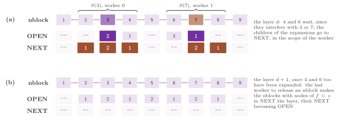
In PSDD (Zhou and Hansen [128]) each nblock has two OPEN lists, OPEN for the current layer and NEXT for the following one, and each child generated in a layer goes into NEXT; hence the layers are those of a breadth-first search, as in the breadth-first heuristic search of Zhou and Hansen [129], on which PSDD is built, and the nodes of \(f\) above a bound \(\beta\) are pruned. A node reached again with a smaller \(g\) goes into NEXT as well, its old entry becoming stale, and it is therefore expanded again in the next layer. In BFPSDD (section 2.4.1 of [3]) NEXT is OPEN, and a layer holds the nblocks whose least \(f\) is the least of all, \(\lambda\), together with others up to \(m p\) nblocks in all, \(m\) being the multiplier (4 by default, the value of [3]); a worker leaves its nblock when the least \(f\) of its OPEN list exceeds \(\lambda\), after a minimum number \(e\) of expansions in it. Figure 12.1 draws a layer of PSDD on the abstract graph of the vacuum world (§11.1).
The two searches are the class template LayeredNBlockSearch, whose
first parameter BestFirst selects BFPSDD, with the two aliases PSDD
and BFPSDD (PSDD.h:191, 664 and 673). Their options
are the following.
struct PSDDOptions : public ParallelOptions {

 /// BFPSDD: the nblocks of a layer are multiplier times the workers, at
 /// least, the ties on the least f all included; 4 is the value of
 /// section 2.4.1 of Burns et al. (JAIR 2010)
 double multiplier = 4;

 /// BFPSDD: the expansions in an nblock before its worker may leave it
 /// for a node of f above the value of the layer
 unsigned min_expansions = 32;

 /// IDPSDD: the growth of IDA*-CR, the bounds being the least f pruned if
 /// not above 1 [see Deepening.h]; every path found is optimal anyway,
 /// since PSDD finds the best path within its bound
 double growth = 0;

 PSDDOptions( void ) = default;

 /// the options of the parallel searches, with the defaults of BFPSDD
 PSDDOptions( const ParallelOptions & o ) : ParallelOptions( o ) {}

 };  // end( struct( PSDDOptions ) )
The fields multiplier (\(m\), taken as 4 if not positive) and
min_expansions (\(e\), taken as 1 if 0) are read by BFPSDD only, and
growth by IDPSDD (below); of the inherited fields, threads is \(p\) and
node_limit bounds the nodes stored by each worker, while batch,
flush_period and seed are not used.
The algorithm¶
The pseudocode of the library (the Doxygen comment of
PSDD.h) is the following, with \(z\) the incumbent, \(\beta\) the
bound given to solve() (\(\infty\) by default), \(\lambda\) the value of the
layer of BFPSDD, \(b(v) = \phi(v)\) the nblock of \(v\), and the conventions
of §1.4.
Algorithm 12.1 (PSDD and BFPSDD).
 1  procedure THREADSEARCH()                        ▷ on each worker
 2     b ← nil
 3     loop
 4        b ← NEXTNBLOCK(b);  if b = nil then return
 5        k ← 0
 6        while OPEN(b) has a node of f < z do
 7           if BFPSDD, k ≥ e and the least f of OPEN(b) is above λ then
               break
 8           u ← the first node of OPEN(b), removed;  close u;  k ← k + 1
 9           for each successor v of u, g' ← g(u) + c(u, v) do
10              if g' + h(v) > β or g' + h(v) ≥ z then continue
11              if v ∉ CLOSED(b(v)) or g' < g(v) then
12                 g(v) ← g';  parent(v) ← u;  v is not closed
13                 if v is a goal then z ← min(z, g'), recording v
14                 else push v in NEXT(b(v))
15  procedure NEXTNBLOCK(b)
16     lock the graph
17     if b ≠ nil then release b, freeing the nblocks of the layer
          that no nblock in use interferes with any more
18     while no nblock of the layer is free do
19        if no nblock is in use then NEXTLAYER()
20        if done then return nil
21        if some nblock is in use then sleep until woken
22     b ← a free nblock of the layer;  acquire b;  return b
23  procedure NEXTLAYER()
24     if PSDD then
25        the layer: the nblocks with nodes of f < z in NEXT, whose
             NEXT becomes OPEN
26     else
27        λ ← the least f < z of the OPEN lists
28        the layer: the m p nblocks of least f < z in OPEN, and all
             those whose least f is λ
29     if the layer is empty then done ← true
30     wake all
Line 10 prunes by the bound and by the incumbent; the \(f\) of the nodes
pruned by the bound are kept, for IDPSDD, in a CutoffHistogram (section
12.6). The goal test is made at the generation (line 13), and a goal is
never pushed: it only lowers \(z\), and the search goes on until no OPEN
list holds a node of \(f < z\) (line 29), which gives a path of least cost
within the bound whatever the costs of the edges (Theorem 12.4). This is a
departure from the scheme of Zhou and Hansen, in which the first goal ends
the search and the path is optimal only when the edges have the same cost
(cf. section 2.4.1 of [3]). The
acquisition and the release of lines 17 and 22 are those of Algorithm 11.3
without the hot nblocks: an nblock of the layer is free when it is not
in use and \(\sigma = 0\); the release decrements \(\sigma\) on the
interference scope and frees the nblocks of the layer that reach \(\sigma
= 0\) with nodes in their list of the layer; and the acquisition increments
\(\sigma\) on the interference scope of the nblock taken, whose nblocks stop
being free (PSDD.h:369-400). In PSDD, line 25 swaps the
roles of the lists OPEN and NEXT of each nblock (the code keeps two lists
per nblock and the index of the layer,
PSDD.h:424-468), and empties the lists NEXT that hold
only nodes of \(f \ge z\).
Analysis¶
We first show that the lists have one writer at a time, as in Safe PBNF, and then that the end of the search is exact; the optimality follows.
Definition 12.1 (The best path within a bound). For a bound \(\beta\), a path from \(s_0\) is within \(\beta\) if each of its nodes \(v\) has \(g_P(v) + h(v) \le \beta\), \(g_P(v)\) being the cost of the path up to \(v\), and \(C^*_\beta\) is the least cost of a path within \(\beta\) from \(s_0\) to a goal (\(\infty\) if there is none).
Note that \(C^*_\beta \ge C^*\), and that \(C^*_\beta = C^*\) when \(\beta \ge C^*\), since by admissibility each node \(v\) of an optimal path \(P\) has \(g_P(v) + h(v) \le g_P(v) + h^*(v) = C^*\).
Lemma 12.2 (Exclusive access). At each instant at which the lock of the graph is free, (a) \(\sigma(n)\) is the number of the nblocks in use in \(I(n)\), (b) each free nblock is not in use and has \(\sigma = 0\), and (c) no two nblocks in use interfere. Hence the lists OPEN, NEXT and CLOSED of an nblock \(n\) are written by at most one worker at a time, the one that holds the nblock \(c\) with \(n \in S(c)\).
Proof. (a) is the argument of Lemma 11.7 (a): the acquisition and the release of \(b\) change \(\sigma\) by one on \(I(b)\) exactly when \(b\) starts and stops being in use. (b) An nblock becomes free only at line 17, when its \(\sigma\) reaches 0 and it is not in use, or at line 25 or 28, when no nblock is in use and hence \(\sigma \equiv 0\) by (a); it stops being free when it is acquired, or when an nblock of its interference scope is acquired, since each acquisition clears the flag free of the nblocks whose \(\sigma\) it raises. (c) An nblock is acquired only when it is free, i.e., by (b) and (a), when no nblock of its interference scope is in use. The last claim is Theorem 11.8, whose proof uses only (a), (c) and the fact that the children of the nodes of \(c\) lie in \(S(c)\) (Lemma 11.3). \(\square\)
Lemma 12.3 (The end of a layered search). When
done is set at line 29, no OPEN or NEXT list holds an entry that is not
stale and has \(f < z\), and no worker holds an nblock.
Proof. Line 29 runs within line 19, i.e., when no nblock is in use,
under the lock of the graph. We first show that each nblock with an
entry that is not stale in the list from which the next layer is built
(NEXT in PSDD, OPEN in BFPSDD) is among the candidates that line 25 or
28 examines. An entry pushed into such a list that was empty, of an
nblock that is not a candidate, makes the worker record the nblock, and
the worker makes it a candidate under the lock of the graph at its next
call of NEXTNBLOCK (PSDD.h:549-555 and 628-631); since
no nblock is in use at line 19, each worker has made that call since its
last insertion. In BFPSDD, moreover, an nblock released with nodes left
in OPEN, and an nblock with nodes of \(f < z\) that line 28 leaves out of
the layer, are made candidates again (PSDD.h:383-391
and 455-464). NEXTLAYER then empties the lists whose least \(f\), the
stale entries dropped first, is not below \(z\), and makes a layer of all
the others, unless there is none. In PSDD each list OPEN of the finished
layer is empty as well: each nblock of the layer with nodes in it is
free or blocked by an nblock in use, a blocked one is freed by the
release that brings its \(\sigma\) to 0 (line 17), and the layer ends only
when none is free and none is in use, i.e., when each of them has been
acquired and its list consumed, or emptied at line 6 because its least
\(f\) is not below \(z\) (PSDD.h:519-545). Hence, when the
layer is empty, no list holds an entry that is not stale with \(f < z\).
\(\square\)
The goal test of PSDD is at the generation, unlike that of the searches of Chapter 8, and we therefore prove the optimality directly, along the lines of Theorem 8.6.
Theorem 12.4 (Optimality within the bound). Let
\(h\) be admissible and let solve( β ) of PSDD or BFPSDD end without
reaching the node limit. Then it returns a path of cost \(C^*_\beta\)
within \(\beta\), or the status unsolvable if \(C^*_\beta = \infty\). In
particular, with \(\beta \ge C^*\) (e.g., with no bound) the path is
optimal.
Proof. If \(h(s_0) > \beta\) or \(s_0\) is a goal, solve() returns at
once with the status unsolvable or the path \((s_0)\)
(PSDD.h:268-274), which is right. Otherwise, we first
show that \(z \le C^*_\beta\) at the end. Suppose not, and let \(P = (w_0 =
s_0, \ldots, w_m)\) be a path within \(\beta\) to a goal, of cost
\(C^*_\beta\), with no goal before \(w_m\) (a goal \(w_j\) with \(j < m\) would
give a cheaper path within \(\beta\)). Call \(w_i\) reached if at some
instant its node has \(g \le g_P(w_i)\). Clearly, \(w_0\) is reached, and if
\(w_m\) is reached then an insertion of line 11 gave it \(g \le C^*_\beta\)
and line 13 set \(z \le C^*_\beta\), or line 10 skipped it because \(g' +
h(w_m) \ge z\), which with \(h(w_m) = 0\) (by admissibility) again means
\(z \le C^*_\beta\). Let \(i \ge 1\) be the least index such that \(w_i\) is not
reached, and let \(\gamma \le g_P(w_{i-1})\) be the least value that the
\(g\) of \(w_{i-1}\) ever takes. The node of \(w_{i-1}\) received \(\gamma\) at
line 12 (or is the root, with \(\gamma = 0\)) and was pushed with it at line
14 (it is not a goal), and that entry becomes stale only by the expansion
of the node with \(g = \gamma\), since \(g\) never decreases below \(\gamma\).
Its key is \(\gamma + h(w_{i-1}) \le g_P(w_{i-1}) + h^*(w_{i-1}) \le
C^*_\beta < z\), where \(h^*(w_{i-1}) \le C^*_\beta - g_P(w_{i-1})\) since the
rest of \(P\) is a path to a goal. By Lemma 12.3 the entry is not in a
list at the end, and a list is emptied at line 6 or 25 only when its least
\(f\) is not below the incumbent of that instant, which is at least the
final \(z\); hence the entry was expanded. Its expansion generated \(w_i\)
with \(g' \le \gamma + c(w_{i-1}, w_i) \le g_P(w_i)\), which line 10 did not
prune, since \(g' + h(w_i) \le g_P(w_i) + h(w_i) \le \beta\) (\(P\) is within
\(\beta\)) and \(g' + h(w_i) \le C^*_\beta < z\); then line 11 found its node
with \(g \le g'\) or gave it \(g'\), and \(w_i\) is reached, a contradiction.
Conversely, \(z\) is the \(g\) of the recorded goal, and the path rebuilt from
it through the parents is within \(\beta\). Indeed, each node of the chain
was pushed or recorded with a value of \(g\) that passed line 10, and its
\(g\) has only decreased since; along the chain \(g(v) \ge
g(\mathrm{parent}(v)) + c(\mathrm{parent}(v), v)\) holds at the end, since
the \(g\) of a parent only decreases after it is used (cf. the proof of
Theorem 11.12). Hence the cost of the chain up
to each of its nodes \(v\) is at most \(g(v)\), and its \(f\) along the chain is
at most \(g(v) + h(v) \le \beta\); the chain is a path within \(\beta\) to a
goal, of cost at most \(z\), and therefore \(C^*_\beta \le z\). Hence \(z =
C^*_\beta\), and the path returned costs exactly \(C^*_\beta\). If no goal is
recorded, \(C^*_\beta = \infty\) by the first part, and the status is
unsolvable. \(\square\)
With unit costs PSDD ends with the layer of the first goal, as the scheme of Zhou and Hansen does, which the following corollary makes precise.
Corollary 12.5 (Unit costs). If each edge costs 1, the layer \(d\) of PSDD holds the nodes of \(g = d\), no node is reopened, and a goal generated in the layer \(d\) ends the search when the layer \(d + 1\) is built.
Proof. By induction on \(d\): the layer 0 holds the root, and the children of the nodes of \(g = d\) have \(g = d + 1\) and go into NEXT; a node reached again has a \(g\) not smaller than its first one, which with unit costs is its depth in breadth-first order, so that no node is reopened. A goal generated in the layer \(d\) gives \(z = d + 1\), and each node pushed into NEXT in the layer \(d\) has \(f \ge g = d + 1 = z\); hence line 25 finds no node of \(f < z\), and the layer is empty. \(\square\)
We remark that the scheme of Zhou and Hansen stops at the goal, before
the rest of the layer \(d\), while PSDD also expands the rest of that
layer. The page on parallel A\(^*\) of the documentation of the library
(docs/theory/parallel-astar.md) reports that on the
instance 55 of Korf with \(\beta = 41\) the two expand the same 199 299 nodes, a
count that we have not rerun.
The bounds of PSDD¶
A bound is what makes PSDD practical: without it, PSDD with an admissible \(h\) expands each node of \(f < z\) layer by layer, and \(z\) is known only when a goal is generated, i.e., late; the bound prunes the nodes of large \(f\) from the start. The library gives the bound in two ways, both of Burns et al. (section 2.4.1 of [3]).
IDPSDD (PSDD.h:694) starts from \(\beta = h(s_0)\) and,
after each iteration that finds no path, raises \(\beta\) to the least \(f\)
that the iteration pruned (the bounds of IDA\(^*\),
§4.4), or, with growth \(r > 1\), to the
bound of IDA\(^*\)-CR of Sarkar et al. [132],
which CutoffHistogram computes from the \(f\) of the pruned nodes (section
12.6). The Solution sums the counters of the iterations, but stored,
which is the largest number of nodes of an iteration, and one executor
serves all the iterations.
Theorem 12.6 (IDPSDD). Let \(h\) be admissible and
the state space finite. Then IDPSDD ends, if it does not reach the node
limit, with an optimal path or with the status unsolvable when no goal
is reachable, whatever the rule of its bounds (the least \(f\) pruned or
IDA\(^*\)-CR).
Proof. Each iteration is a solve( β ) of PSDD, which ends on a finite
space (Proposition 12.8 below). An iteration with \(\beta < C^*\) finds no
path, since a path within \(\beta\) to a goal costs at most \(\beta\) (\(h\) is
0 at a goal); and if a goal is reachable, it prunes a node of \(f \le C^*\):
the argument of the proof of Theorem 12.4, applied to an optimal path
\(P\), gives a first node of \(P\) that is not reached, which is generated
with \(f \le g_P + h \le C^*\) and pruned by the bound, since \(z = \infty\)
in that iteration. Both rules give a next bound not smaller than the least
\(f\) pruned, which exceeds \(\beta\) (Deepening.h:200);
since the values of \(f\) of a finite space are finitely many, after
finitely many iterations either \(\beta \ge C^*\), and then Theorem 12.4
gives a path of cost \(C^*_\beta = C^*\), or no node is pruned and the
iteration ends with no path, which IDPSDD returns as unsolvable. By the
remark above, the latter happens only when no goal is reachable. \(\square\)
Unlike IDA\(^*\) (section 12.6), IDPSDD needs no completion of the iteration
that finds the first path, since PSDD already finds the best path within
its bound, and a bound above \(C^*\) costs only the nodes of \(f\) between
\(C^*\) and the bound. This is why IDA\(^*\)-CR is safe for IDPSDD with any
growth, and why its option growth is described as giving optimal paths
anyway.
DynamicBoundedPSDD (PSDD.h:795) takes the bound from a
first search. A\(^*\) (Chapter 2) on the Domain
whose heuristic is \(w h\) (\(\lfloor w h \rfloor\) with integer costs; the
class Inflated of PSDD.h:857, which hands to the
successors of the original Domain the original \(h\) of the parent, as a
Domain that computes its heuristic incrementally needs), with the weight
\(w \ge 1\) given to the constructor (1 if smaller), finds a path of cost
\(c\), and PSDD with \(\beta = c\) then finds an optimal path.
Proposition 12.7 (DynamicBoundedPSDD). Let \(h\)
be admissible. If the first search ends with a path, DynamicBoundedPSDD
returns an optimal path (unless PSDD reaches the node limit); otherwise
it returns the status of the first search (unsolvable or
node_limit).
Proof. The cost \(c\) of the path of the first search is the cost of a path of the graph, hence \(c \ge C^*\), and PSDD with \(\beta = c \ge C^*\) returns a path of cost \(C^*_c = C^*\) by Theorem 12.4. Since the two searches search the same graph, a first search that proves no goal reachable is right. \(\square\)
Note that the proof uses only \(c \ge C^*\); the bound \(c \le w C^*\) of
weighted A\(^*\) (Pohl [46] and Chapter
6) serves only to keep the second search
small, since the nodes of \(f \le c\) grow with \(c\), and hence with \(w\). The
documentation reports that on the instance 55 of Korf \(w = 1.5\) gives \(c
= 47\) against \(C^* = 41\) (a count that we have not rerun). The counters of
the Solution are those of the two searches summed, but stored, the
larger of the two.
Proposition 12.8 (Termination). On a finite
state space, solve( β ) of PSDD and BFPSDD ends, under any scheduling in
which a worker that can proceed eventually does.
Proof. A node is pushed only when its \(g\) takes a new, strictly
smaller value, the cost of a simple path (cf. Theorem
11.13); hence the pushes, and the expansions,
are finitely many. Each acquisition is followed by at least one
expansion or by the emptying of a list, since an nblock of a layer is free
only with nodes in its list of the layer, and in BFPSDD \(e \ge 1\) lets the
worker expand at least one node; hence the acquisitions are finitely many,
and so are the layers, each of which removes at least one entry. A worker
sleeps at line 21 only while an nblock is in use, whose worker reaches
its release in finite time and wakes the sleepers when it frees an nblock
or builds a layer, under the same lock; hence no worker sleeps forever,
and the last layer, the empty one, sets done and wakes all. \(\square\)
The engineering¶
The nblocks are those of Safe PBNF, built at their first use by the
class template NBlockMap of NBlockMap.h, which the two
searches share (§11.7 describes it); an nblock
of PSDD holds its two lists OPEN and NEXT (one list in BFPSDD), its table
of nodes, its scopes, \(\sigma\), and the flags in use, free, in the layer
and candidate (PSDD.h:332-342). The free nblocks of a
layer are a vector, which a worker scans from its end, skipping the
entries whose flag free an acquisition has cleared (an acquisition clears
the flags of the nblocks of the interference scope without searching the
vector); the candidates of the next layer are a vector of their own, and
BFPSDD sorts them by their least \(f\) at line 28. The lock of the graph is
a std::mutex rather than the lock of the executor
(PSDD.h:325): at the end of a layer all the workers but one
wait while the last one builds the next layer, and with the spin lock of
an executor they would spin for the whole of that time. The expansion is
that of Safe PBNF (Algorithm 11.6): the successors are generated and their
slots prefetched first, and looked up afterwards; the nodes are allocated
from an arena of each worker; the goal is recorded under a separate
mutex; and the incumbent is read with relaxed order at line 10, which may
only prune less. The cost of a layer is that of its expansions, plus one
critical section per acquisition and the barrier, i.e., the time between
the first worker that finds no free nblock and the last release. When
the layers are small, as the layers of \(f\) of BFPSDD on a domain with many
distinct values of \(f\), the barrier typically dominates, which is why Burns et al.
introduced PBNF (section 2.4.1 of [3], p. 696,
and §11.2).
12.3 K-best-first search¶
KBFS of Felner, Kraus and Korf [130]
expands, at each step, the \(K\) best nodes of OPEN, and inserts all their
children before the next step; with \(K\) processors the expansions of a
step run in parallel. In the library it is the farm of
§8.7 with the option synchronous of
FarmOptions:
struct FarmOptions : public ParallelOptions {

 /// true for the synchronous rounds of KBFS: the master sends a task to
 /// each worker, waits for all of them and inserts their successors in the
 /// order in which it sent them before the next round
 bool synchronous = false;

 FarmOptions( void ) = default;

 /// the options of the parallel searches, without rounds
 FarmOptions( const ParallelOptions & o ) : ParallelOptions( o ) {}

 };  // end( struct( FarmOptions ) )
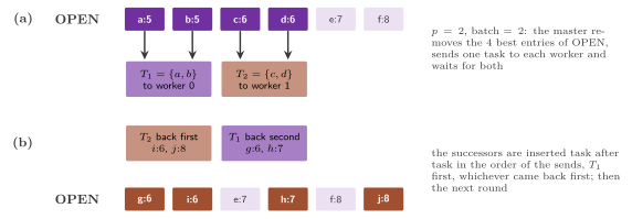
With it the farm runs in rounds: the master sends a task of up to
batch nodes to each of the \(p\) workers, which are all free at the start
of a round, waits until each task is back, and only then inserts the
successors, task after task in the order in which it sent them, before it
dispatches the next round; thus \(K = p \cdot \mathrm{batch}\). DISPATCH
(Algorithm 8.6) is unchanged, and the return of a task (Algorithm 8.7)
becomes the following (FarmAStar.h:261-279).
Algorithm 12.2 (The return of a task in the rounds of KBFS, on the master; \(R\) is the list of the tasks of the round, in the order of the sends, to which DISPATCH appends).
 1  function BACK(T)
 2     out ← out − 1
 3     if out > 0 then return true           ▷ the round is not over
 4     for each task T' of R, in order, do
 5        insert the successors of the nodes of T' as Algorithm 8.7 does
 6     R ← ∅
 7     if the master stores at least node_limit nodes then the limit is hit
 8     DISPATCH()                            ▷ the next round, appended to R
 9     return out > 0 or (the limit is not hit and OPEN has a node of f < z)
Figure 12.2 draws one round. The search is deterministic: the order of the insertions, and hence the breaking of the ties in OPEN, no longer depends on the order in which the workers finish.
Proposition 12.9 (KBFS). Let \(h\) be admissible
and the generation of the successors by the Domain deterministic. (i)
KBFS returns an optimal path if it ends without reaching the node limit,
and it ends on a finite graph. (ii) Its expansions, its counters and its
path are the same at each run, whatever the scheduling of the workers.
(iii) With one worker and tasks of one node it expands the nodes that
A\(^*\) expands with the same OPEN list, in the same order.
Proof. (i) The rounds only delay the insertions: the invariant of out (Lemma 8.17) holds whenever the master is between two of its steps, with the tasks of the round that have come back counted among those that are out until their successors are inserted (the master keeps them in \(R\) and inserts nothing before the round is over); hence the proof of Theorem 8.18 applies. (ii) The master is the only thread that changes OPEN, CLOSED, \(z\) and the nodes, and its steps are DISPATCH, which depends only on its state, and the insertion of a round, which depends only on the tasks of \(R\), in the order of the sends, and on their successors, which are a function of the nodes of each task. By induction on the rounds, the state of the master after each round is the same at each run. (iii) With \(p = 1\) and batch 1, each round sends the first node of OPEN of \(f < z\), after recording as the incumbent the goals that come first (the goal test of DISPATCH), and inserts its successors before the next selection, which is the loop of A\(^*\) with the goal test at the selection. A\(^*\) stops at the first goal it selects, of cost \(C^*\); the master records it as \(z = C^*\), and since that goal was the first entry of OPEN, no entry left has \(f < z\), so that the master stops there too. \(\square\)
The test farm-thread checks (iii) on an instance of Korf (the counters
expanded of KBFS and of astar() are equal) and (ii) with 2, 3 and 8
workers and tasks of 2 nodes (two runs with the same expansions and
generations). The price of the determinism is the barrier of each round,
which leaves idle the workers that finish first; Burns et al. found that
KBFS does not beat serial A\(^*\) on their grids (section 2.1 of
[3]), and we expect it to pay, if at
all, only when the expansions are slow and of similar cost.
12.4 A portfolio of A* searches¶
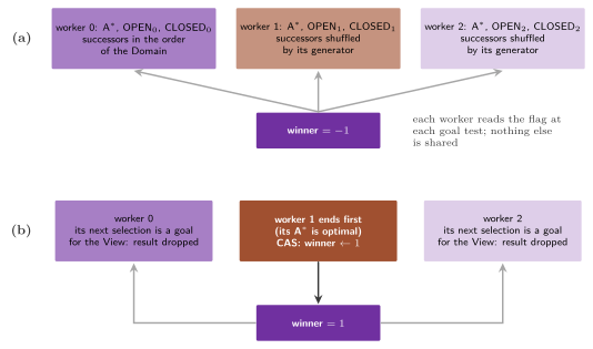
The simplest parallel search shares nothing but a flag: MultiAStar
(MultiAStar.h:73) runs \(p\) independent A\(^*\)
searches, with the options given (the weight included), and the first one
to end gives the Solution. The worker 0 runs the plain A\(^*\); the worker
\(i > 0\) runs it on a view of the Domain (the struct View,
MultiAStar.h:143) that generates the successors of
each state in an order drawn by a generator of its own (a Fisher-Yates
shuffle on a xorshift generator, seeded by splitmix64 of the seed of
the options and of \(i\)), so that the nodes of equal \(f\) and \(g\) enter its
OPEN list in another order and the ties are broken otherwise. The view
also makes each state a goal once the flag is set, so that the next
selection of each other worker ends its search, whose result is dropped.
Algorithm 12.3 (Multi-A\(^*\); winner is atomic, \(-1\) at the start).
 1  procedure MULTI-A*(s₀, p)
 2     winner ← −1
 3     in parallel, on each worker i = 0, ..., p − 1 do
 4        S_i ← A* on the view V_i, whose goal test is
             "winner ≥ 0 or the state is a goal"
 5        if winner = −1 then winner ← i      ▷ a compare-and-swap
 6     return S_winner, with the counters of all the workers summed
Figure 12.3 draws the portfolio.
Proposition 12.10 (Multi-A\(^*\)). The
Solution of MultiAStar is that of an A\(^*\) search on the Domain with
the options given, and hence it has the guarantees of A\(^*\) (Chapter
2, or Chapter 6
with a weight); with one worker its expansions are those of astar().
Proof. The winner is the worker whose compare-and-swap of line 5 found
\(-1\). Its search never read winner \(\ge 0\), since winner never returns to
\(-1\) once set, and a worker that has read it set finds it set at line 5;
hence each goal test of the winner was the goal test of the Domain,
and its search is A\(^*\) on the graph of the Domain with the order of the
successors of its view, which changes nothing else. With \(p = 1\) the view
of the worker 0 forwards the successors in the order of the Domain.
\(\square\)
We expect the portfolio to pay, if at all, only when the expansions of A\(^*\) in the last layer of
\(f\) depend much on the ties, which the preference for the larger \(g\)
already reduces (§2.8), at the price of \(p\)
times the memory and of a memory bus shared by \(p\) searches that usually do
much the same work. The node limit holds for each worker, and the status
node_limit of the first worker to reach it ends the portfolio, even if
another worker would have solved the instance. The counters expanded_by
and stored_by hold those of each worker, and the test multi-thread
checks that one worker expands as astar().
12.5 Synchronous messages and the lending of nodes¶
Two options of HDAStar change the communication of HDA\(^*\) (Chapter
9), and a family of channels changes the way
in which a worker receives:
struct HDAOptions : public ParallelOptions {

 /// true to push every node to its owner as soon as it is generated, as
 /// in PRA*, instead of packing the nodes in batches
 bool sync_send = false;

 /// if positive, a worker lends the node it is about to expand to the
 /// worker whose best f is the least among those not smaller than its f
 /// plus outsource, which expands it at once; 0 for none
 double outsource = 0;

 HDAOptions( void ) = default;

 /// the options of the parallel searches, with no synchronous send and no
 /// lending
 HDAOptions( const ParallelOptions & o ) : ParallelOptions( o ) {}

 };  // end( struct( HDAOptions ) )
template< ADS::WorkerExecutor Executor >
struct LockedChannelsOf {
 /// the family for the messages Msg
 template< class Msg >
 using type = ADS::LockedChannels< Msg , typename Executor::lock_type >;
 };  // end( struct( LockedChannelsOf ) )
PRA* and APRA*¶
PRA\(^*\) of Evett et al. [127] is the
ancestor of HDA\(^*\): each state has an owner by a hash, and a node is sent
to its owner when it is generated. On the massively parallel machine for
which it was written the communication was synchronous at both ends, and
a worker whose memory filled up retracted its worst nodes, i.e., removed
them and kept in their parents the least \(f\) of what it removed. Burns et
al. separated the two halves of the communication, compared the four
combinations of synchronous and asynchronous sends and receives, and
called APRA\(^*\) the variant whose owner is given by an abstraction
[3]. The library has the two
synchronous halves, without the retraction. With sync_send the mailbox
of HDAStar has batches of one node
(HDAStar.h:267), so that each node is pushed to its
owner as soon as it is generated; with the channels LockedChannelsOf<
Executor > an inbox is a vector under the lock of the executor, which the
receiver takes, waiting for it, to receive. The two together are
PRA\(^*\), and with the AbstractStateDistribution of Chapter
9 they are APRA\(^*\). Since only the
transport of the messages changes, HDA\(^*\) keeps its correctness and its
termination (§9.3): the deficit counting
counts each message, whatever its size, and the test hda-thread runs
PRA\(^*\), APRA\(^*\) and the two halves alone on an instance of Korf.
The lending of nodes¶
A distribution of the states balances the nodes among the workers, not
the nodes of small \(f\): a worker may hold the best nodes of the search
while another expands nodes that A\(^*\) would never select (the band
effect of §8.2). With outsource \(=
\delta > 0\), each worker publishes, before each expansion, the \(f\) of
the node that it is about to expand (\(\infty\) when it has none), and the
worker \(i\) that is about to expand \(u\), not a goal, lends it to the
worker \(j\) whose published value is the least among those not smaller
than \(f(u) + \delta\), if there is one
(HDAStar.h:434-466). The borrower expands the node
as soon as it receives it and sends its successors to their owners, while
the node stays in the CLOSED list of its owner; a lent node is never lent
again.
Algorithm 12.4 (The lending of HDA\(^*\), on the worker \(i\) that has selected \(u\); \(F_j\) is the value published by the worker \(j\)).
 1  procedure STEP(u)                  ▷ u selected at line 7 of HDA*
 2     F_i ← f(u)
 3     j ← the worker j ≠ i of least F_j among those with F_j ≥ f(u) + δ
 4     if there is none or u is a goal then expand u as HDA* does;  return
 5     close u;  send (u, g(u), lent) to j;  flush the outbox to j
 6  procedure RECEIVE(u, g, lent)       ▷ on the borrower j
 7     if g + h(u) ≥ z then return
 8     for each successor v of u, g' ← g + c(u, v), with g' + h(v) < z do
 9        if owner(v) = j then INSERT(v, g', u) else send (v, g', u) to owner(v)
Proposition 12.11 (HDA\(^*\) with lending). With
outsource positive, with or without sync_send and the locked
channels, HDA\(^*\) is well-formed in the sense of
§8.3; hence, if it ends without reaching
the node limit, it returns an optimal path.
Proof. We check the conditions of §8.3 for the entry of a lent node, the others being those of HDA\(^*\). The entry of \(u\), selected by its owner, leaves OPEN at line 7 of HDA\(^*\) and is closed at line 5; from then on it is in the message to \(j\) (condition (iii) of Definition 8.5), and then held by \(j\) until \(j\) has inserted or sent each successor (condition (ii)); the mailbox counts the message, so that the end of the search is not detected while it travels. The borrower satisfies condition (b): it prunes by a value of \(z\) of the past (lines 7 and 8) and creates, by the insertion or the message of line 9, an entry of each successor with \(g' = g + c(u, v)\), the cost of a path to \(v\) through \(u\), whose parent pointer is the node of \(u\) at its owner. A goal is never lent (line 4), so that condition (c) is that of HDA\(^*\), and Theorem 8.6 gives \(z = C^*\) at the end. Since the borrower only reads the fields of the message and stores the pointer to the node of \(u\), which only its owner writes, the lending adds no data race. \(\square\)
The lending moves work away from a worker whose nodes are much better than
those of the others, which the distribution alone usually cannot do, at the price
of one message per node lent and of the published values, one atomic per
worker on a cache line of its own (HDAStar.h:325). An
idle worker publishes \(\infty\), and therefore receives a node only when no
busy worker is far enough behind; the gap \(\delta\) keeps the workers whose
nodes are about as good from lending to each other. The borrower counts
the expansion of a lent node in its expanded, and the owner counts a
later expansion of the same node, after an improvement of its \(g\), as a
re-expansion. The test hda-thread runs the lending with a gap of 2 on an
instance of Korf and with a gap of 3 and synchronous sends on a grid with
8 moves, and the corner cases of check_astar_edges with PRA\(^*\) and a
gap of 1.
12.6 Transposition-table driven scheduling¶
IDA\(^*\) (§4.4) stores only its path, and on a graph with many transpositions it searches the same subtree once for each path that reaches its root within the bound. TDS of Romein, Plaat, Bal and Schaeffer [131] parallelizes IDA\(^*\) by a transposition table split among the workers by owners, as the CLOSED list of HDA\(^*\) is: each node is sent to the worker that owns the entry of its state, which looks it up there and, if the state is not already being searched in the iteration with a budget at least as large, pushes it on its own stack; each worker searches depth first from its stack. The work moves with the data, so that a lookup never crosses the workers, and the subtree of a state is searched at most once in an iteration.
The algorithm¶
The pseudocode of the library (the Doxygen comment of TDS.h)
is the following, with \(\beta\) the bound of the iteration, \(T_i\) the part
of the table of the worker \(i\), each entry with the \(g\) with which its
state was last pushed in the iteration, and a message \((v, g', u)\) a state
with the cost and the predecessor of its path.
Algorithm 12.5 (TDS).
 1  procedure TDS(s₀, p, owner)
 2     β ← h(s₀)
 3     loop
 4        β' ← ∞;  INSERT(s₀, 0, nil) on owner(s₀)
 5        in parallel, on each worker i, until no worker has work and
             no message is in transit, or a goal is found, do
 6           for each message (v, g', u) received do INSERT(v, g', u)
 7           if the stack of i is not empty then
 8              u ← pop the stack (stale entries dropped)
 9              if u is a goal then record u;  stop all
10              for each successor v of u, g' ← g(u) + c(u, v) do
11                 if g' + h(v) > β then β' ← min(β', g' + h(v))
12                 else if owner(v) = i then INSERT(v, g', u)
13                 else send (v, g', u) to owner(v)
14        if a goal was recorded then return the path to it
15        if β' = ∞ then return unsolvable
16        β ← β'
17  procedure INSERT(v, g', u)                       ▷ on the owner i of v
18     if T_i has v from this iteration with g(v) ≤ g' then return
19     g(v) ← g';  parent(v) ← u;  push v on the stack of i
Line 18 is what TDS adds to IDA\(^*\): since the bound is the same for the
whole iteration, a state already pushed in it with a \(g\) not larger has
been, or is being, searched with a remaining budget \(\beta - g\) at least
as large, and its subtree is not searched again by any worker (Romein et
al., p. 3 of [131]). An entry of the stack is
the pair of the node and of the \(g\) with which it was pushed, and it is
stale if the \(g\) of the node has changed since (line 8,
TDS.h:326-335). The entries of the table are nodes kept
from an iteration to the next and marked with the iteration that last
pushed them (TDS.h:383-408), so that the table holds
each state generated within the bounds, as the CLOSED list of A\(^*\)
does, and no subtree is searched twice in an iteration (the case of a
table "large enough" in [131], which does not
replace its entries); the node limit, per worker, bounds the table. Each
iteration is a computation of the mailbox of Chapter
9, whose end, i.e., no worker with work
and no message in transit, is detected by its deficit counting
(§9.3); the nodes travel in batches,
the outboxes being flushed each flush_period expansions and before a
worker waits, and the least \(f\) pruned is the least over the workers, read
after the iteration. The class template is TDS< D , Dist , Executor >,
the distribution Dist being one of those of
§9.4 (by default the hash of the state),
and its options are the following.
struct TDSOptions : public ParallelOptions , public DeepeningOptions {

 TDSOptions( void ) = default;

 /// the options of the parallel searches, with the classical bounds
 TDSOptions( const ParallelOptions & o ) : ParallelOptions( o ) {}

 };  // end( struct( TDSOptions ) )
The fields of DeepeningOptions (Deepening.h) are those
of the bounds of IDA\(^*\)-CR, which IDA\(^*\) shares (§4.4
describes them for the sequential search): growth \(r\) (0 by default, the
classical bounds) and optimal (true by default). Of the inherited fields,
threads, batch, flush_period and node_limit are read, while the
weight is ignored.
Analysis with the classical bounds¶
We call an iteration classical when it is not completed as a
branch-and-bound, i.e., when the first goal found stops it (line 9); with
growth at most 1 each iteration is classical.
Lemma 12.12 (The optimal path in an iteration). Let \(h\) be admissible, let \(P = (w_0 = s_0, \ldots, w_m)\) be an optimal path to a goal with no goal before \(w_m\), and consider an iteration of bound \(\beta\) in which no goal is found and the node limit is not reached. Then for some \(j \ge 1\) the state \(w_j\) is generated with \(g' \le g_P(w_j)\) and pruned at line 11, with \(f = g' + h(w_j) \le C^*\), while \(w_0, \ldots, w_{j-1}\) are pushed in the iteration with \(g\) not larger than \(g_P\); and if \(\beta \ge C^*\), a goal is found in the iteration.
Proof. We show by induction on \(i\) that, as long as \(w_i\) is not pruned, it is pushed in the iteration with \(g \le g_P(w_i)\), and expanded with the least \(g\) with which it was pushed. For \(i = 0\) the root is inserted at line 4 with \(g = 0\). If \(w_i\) is pushed with \(g \le g_P(w_i)\), let \(\gamma\) be the least \(g\) with which it is pushed in the iteration; the entry of \(\gamma\) is never stale, since within an iteration the \(g\) of a node only decreases (line 18 rejects the larger values), and since the iteration ends only when no worker has work and no message is in transit, the entry is popped and expanded with \(g = \gamma\) (the incumbent does not prune in a classical iteration). Its expansion generates \(w_{i+1}\) with \(g' \le \gamma + c(w_i, w_{i+1}) \le g_P(w_{i+1})\) and \(f = g' + h(w_{i+1}) \le g_P(w_{i+1}) + h^*(w_{i+1}) = C^*\); if \(f > \beta\), it is pruned at line 11, and otherwise it reaches its owner, which either finds it pushed in the iteration with \(g \le g'\) (line 18) or pushes it with \(g'\) (line 19). If no state of \(P\) were pruned, the goal \(w_m\) would be expanded, and a goal found. Finally, if \(\beta \ge C^*\), no state of \(P\) is pruned, since each is generated with \(f \le C^* \le \beta\); hence a goal is found. \(\square\)
Theorem 12.13 (TDS with the classical bounds).
Let \(h\) be admissible and the costs positive, and let the bounds be the
least \(f\) pruned (growth at most 1). If TDS ends without reaching the
node limit, the path it returns is optimal; if it returns unsolvable,
no goal is reachable.
Proof. A state is pushed only with \(g + h \le \beta\), so that a goal
found in an iteration of bound \(\beta\) has \(g \le \beta\) (\(h\) is 0 at a
goal). By Lemma 12.12, while \(\beta < C^*\) no goal is found (a goal has \(g
\ge C^*\)) and the least \(f\) pruned is at most \(C^*\); hence the bounds
increase strictly and never skip \(C^*\), and the first iteration in which
a goal is found is the one with \(\beta = C^*\), in which each goal found
has \(g \le C^*\), i.e., \(g = C^*\). The path is rebuilt from the goal
through the parents after the workers have returned; within the
iteration a node's \(g\) and parent are set together at line 19 and the \(g\)
only decreases, so that along the chain the \(g\) of a parent at the end is
at most the value with which it generated its child, and the chain is a
path of cost at most \(C^*\) whose nodes were all pushed in the iteration.
Its cost is recomputed from the Domain, each edge being the cheapest
between two consecutive states (TDS.h:425-438), which
can only lower it; hence it is \(C^*\). Finally, if no goal is reachable,
TDS returns unsolvable only when an iteration prunes nothing (\(\beta' =
\infty\)), which is right. \(\square\)
Note that termination needs, as for IDA\(^*\), that each iteration be
finite and that the bounds reach \(C^*\) in finitely many steps, which holds
on a finite graph (the table makes each iteration finite even on a graph
with cycles, since a state is pushed in an iteration only when its \(g\)
decreases) and with integer costs on an infinite graph with finite
branching; the test tds-thread checks the optimal cost on two instances
of Korf, on 7 states of the 8-puzzle, on a grid with costs from 1 to 3 and
on the map of Romania, and the status unsolvable on a grid split by a
wall.
The bounds of IDA*-CR¶
On a grid with 8 moves, or with costs that are not integers, the values of
\(f\) are many and close, the iterations are as many as the values of \(f\),
and each iteration expands again the nodes of the ones before. IDA\(^*\)-CR
of Sarkar, Chakrabarti, Ghose and De Sarkar
[132] chooses instead a bound beyond which
enough pruned nodes lie. The class template CutoffHistogram
(Deepening.h:117) collects the \(f\) of the nodes pruned
by an iteration of bound \(\beta_k\) in buckets of the binary exponent of
the excess \(f - \beta_k\) (the excesses in \([2^{x-1}, 2^x)\) in the bucket
\(x\), so that the histogram has a fixed size, 2100 buckets, whatever the
costs, and is fine near the bound and coarse far from it), and its
member next( r , E_k ) returns, with \(E_k\) the expansions of the
iteration and \(\ell_k\) the least \(f\) pruned:
- \(\ell_k\), if \(r \le 1\) (the classical bound);
- otherwise, the largest \(f\) of the first buckets that hold at least \((r - 1) E_k\) pruned nodes;
- when even all the pruned nodes are fewer than that and \(E_k\) is less than \(r\) times the expansions of the iteration before, as on a grid, where the children of the last layer of \(f\) are all just above it, the bound plus twice its last step, \(\beta_k + 2(\beta_k - \beta_{k-1})\), so that the steps grow geometrically while the iterations stay small;
and never less than \(\ell_k\) (Deepening.h:181-204).
In TDS each worker keeps its histogram, and the histograms are merged
after the iteration (merge()); IDPSDD does the same with the histograms
of the workers of PSDD. The price of a bound \(\beta_{k+1} > \ell_k\) is
that the first goal found need not be optimal, which the option optimal
corrects.
Theorem 12.14 (TDS with the bounds of
IDA\(^*\)-CR). Let \(h\) be admissible, \(r > 1\), and let TDS end without
reaching the node limit with a path of cost \(c\), found in the iteration
\(k + 1\). If optimal is false, then \(c - C^* \le \beta_{k+1} - \ell_k\),
where \(\ell_k\) is the least \(f\) pruned by the iteration \(k\) (and \(c =
C^*\) if the goal was found in the first iteration). If optimal is true,
\(c = C^*\).
Proof. As in the proof of Theorem 12.13, a goal found in the iteration
of bound \(\beta\) has \(g \le \beta\), so \(c \le \beta_{k+1}\); and the
iteration \(k\), which found no goal, pruned by Lemma 12.12 a node of \(f \le
C^*\), so \(\ell_k \le C^*\). Hence \(c - C^* \le \beta_{k+1} - \ell_k\). With
optimal, an iteration whose bound exceeds the least \(f\) pruned before
is completed as a depth-first branch-and-bound
(TDS.h:195): a goal lowers the incumbent \(z\) (initially
\(\infty\)) instead of stopping the workers, the nodes of \(f \ge z\) are not
pushed and their entries are dropped when popped, and the iteration ends
when no worker has work. In the iteration \(k + 1\) the argument of Lemma
12.12 applies to an optimal path as long as \(z > C^*\), since its states
have \(f \le C^* < z\) and are not pruned by \(z\), and \(\beta_{k+1} \ge c \ge
C^*\) prunes none of them by the bound; hence the iteration does not end
before \(z \le C^*\), i.e., \(z = C^*\). The path is rebuilt from the goal of
cost \(z\) as in Theorem 12.13. An iteration whose bound is the least \(f\)
pruned before (e.g., the first one) is classical, and its first goal is
optimal by the argument of Theorem 12.13, since its bound does not
exceed \(C^*\). \(\square\)
The same bounds serve IDPSDD (Theorem 12.6), which needs no completion,
and the sequential IDA\(^*\), for which §4.4
proves the bound of the cost and the completion. The test tds-thread
checks TDS with \(r = 2\) on a grid with 8 moves and costs from 1 to 3, with
optimal (the cost of A\(^*\)) and without it (a valid path not cheaper
than the optimum); the test psdd-thread checks IDPSDD with \(r = 2\) on a
grid of \(40 \times 30\) cells.
The engineering¶
A worker of TDS (TDS.h:286-419) keeps its part of the
table, a table of nodes with open addressing, its arena of nodes and its
stack, a vector of pairs (node, \(g\)). It polls its inbox, inserting each
node received, and then pops and expands one entry of its stack, inserting
the successors that it owns at once and sending the others, as HDA\(^*\)
does; the parents cross the workers, and they are followed only after all
the workers have returned. The goal is recorded under a mutex, and a
classical iteration stops the mailbox at the first goal. Since each
iteration is a new computation of the mailbox and the table survives it,
the cost of an iteration is that of its expansions and messages, and the
memory is that of the table, which grows with the states generated within
the bounds; TDS is thus a parallel IDA\(^*\) that uses the memory of A\(^*\)
to search each subtree once, and its iterations still expand the nodes of
the iterations before. With one worker the expansions are the same at each
run, which the test checks.
12.7 Parallel iterative deepening below a frontier¶
ParallelIDAStar (ParallelIDAStar.h) parallelizes
the depth-first iterations of IDA\(^*\) in a different way: it first builds
a frontier, a set of open nodes, the units, and then runs the
iterations below the units on the \(p\) workers. Each unit \(u\) keeps a
threshold \(t_u\), initially \(f(u) = g(u) + h(u)\), and its cost-bounded
search with a bound \(\beta \ge t_u\) returns, besides a goal of cost at most
\(\beta\) if one exists below \(u\), the least \(f\) of the nodes that it cuts,
which becomes \(t_u\). The frontier is built by one of three rules
(FrontierRule):
astar: A\(^*\), with reopening, until OPEN holds \(N\) live nodes, as in the AIDA\(^*\) of Reinefeld and Schnecke [55] and in the A\(^*\)+IDA\(^*\) of Bu and Korf [56];breadth: uniform-cost search, by \(g\), until the same, a breadth-first frontier with unit costs;depth: the tree of the least depth with \(N\) leaves, without duplicate detection (a goal is a leaf, never expanded), the work units of the parallel IDA\(^*\) of Sturtevant and of Siag et al. [57].
If the first two rules expand a goal, or empty OPEN, the frontier ends the
search, with the optimal path (A\(^*\) with reopening and an admissible \(h\),
or uniform-cost search with positive costs, select a goal only with its
optimal cost) or with the status unsolvable
(ParallelIDAStar.h:369-463). Two schemes
share the units.
Algorithm 12.6 (Parallel IDA\(^*\) below a frontier, the synchronous scheme and the asynchronous one).
 1  procedure PIDA*(s₀, p, N)
 2     build the units U by the frontier rule (return if it ends the search)
 3     t_u ← f(u) for each u ∈ U
 4     loop                                       ▷ the synchronous scheme
 5        β ← min_u t_u;  if β = ∞ then return unsolvable
 6        A ← {u ∈ U : t_u ≤ β}       ▷ all the units without unit bounds
 7        in parallel, the workers take the units of A
             (by work stealing, or from a shared cursor):
 8           (goal, t'_u) ← DFS(u, g(u), β);  t_u ← t'_u
 9           if goal then stop all the workers;  return its path

 1  procedure AIDA*(s₀, p, N)                    ▷ the asynchronous scheme
 2     build U;  z ← ∞;  Q ← U by increasing t_u
 3     in parallel, each worker repeats until Q = ∅ and no worker searches:
 4        u ← the first unit of Q, removed;  if t_u ≥ z then drop it
 5        (goal, t'_u) ← DFS(u, g(u), t_u) cutting also f ≥ z
 6        if goal then z ← min(z, its cost), recording its path
 7        t_u ← t'_u;  if t_u < z then put u back in Q
 8     return the path of cost z, or unsolvable
In the synchronous scheme each iteration ends at a barrier, whose last
worker computes the thresholds, the next bound and the units of the next
iteration (ParallelIDAStar.h:641-770); in
the asynchronous one there is no barrier, the workers take the units by
increasing threshold, each searched with its own threshold, and a goal of
cost \(z\) prunes each node with \(f \ge z\). The DFS of a unit is that of
IDA\(^*\) (§4.4) with an explicit stack of
the successors not yet tried, the moves back to the parent skipped (by the
operator in an OperatorDomain, with the redundant pairs of moves of a
TreeOperatorDomain, otherwise by comparing the successor with the state
two places back on the path), and the goal test when a node is reached
within the bound (ParallelIDAStar.h:904-1013).
The options are the following.
enum class FrontierRule : std::uint8_t {
 astar ,     ///< A* until OPEN holds the units wanted
 breadth ,   ///< uniform-cost search (by g) until the same
 depth       ///< the tree of the least depth with that many leaves
 };

/*- - - - - - - - - - - - - - - - - - - - - - - - - - - - - - - - - - - - -*/
/// how the units of an iteration are given to the workers

enum class UnitSchedule : std::uint8_t {
 steal ,     ///< a range of units per worker, half stolen when it is empty
 shared      ///< one cursor over the units, shared by all the workers
 };
struct PIDAOptions : public ParallelOptions {

 /// the units wanted (0: 128 per worker)
 std::size_t frontier = 0;

 /// the rule that builds the frontier
 FrontierRule rule = FrontierRule::astar;

 /// the scheduling of the units of an iteration
 UnitSchedule schedule = UnitSchedule::steal;

 /// a unit is searched only when the bound reaches its threshold; false
 /// searches every unit at every bound
 bool unit_bounds = true;

 /// no barrier between the iterations: the units are searched by
 /// increasing threshold, each with its own (AIDA*)
 bool asynchronous = false;

 /// with a value s > 0, a worker that sees an idle one gives it half of
 /// the successors not yet tried at the shallowest level of its stack,
 /// those whose f is at least s below the bound; 0 disables the splitting
 double split = 0;

 /// the levels below a unit whose nodes are looked up in the table of the
 /// frontier, and pruned if found there with a g not larger
 unsigned table_depth = 0;

 /// the path found is that of the first goal in the order of the units,
 /// the same at every run
 bool deterministic = false;

 };  // end( struct( PIDAOptions ) )
The field frontier is \(N\) (0 gives 128 per worker); unit_bounds
selects line 6 as written, and false searches each unit with a finite
threshold at each bound, the classical scheme; asynchronous selects the
second scheme; split and table_depth are described below. Of the
inherited fields, threads and node_limit are read (the latter bounds
the expansions of each worker in the iterations), while batch and
flush_period are not; the constructor throws std::invalid_argument for
a weight other than 1, for deterministic with the asynchronous scheme or
with splitting, for a table with the rule depth, which has no table, and
for a negative split (ParallelIDAStar.h:238-256).
parallel_idastar( d , o ) runs the search on the default executor, and
iterations() and units() give the iterations (in the asynchronous
scheme, the searches of units) and the units of the last solve().
Optimality¶
The proofs rest on one unit, which keeps a threshold not above \(C^*\)
until an optimal goal is found below it. We assume that the frontier was
built by the rule astar or breadth and did not end the search, and
that the tree pruning of the DFS (the moves back to the parent and the
redundant pairs of moves of a TreeOperatorDomain) leaves, from each
state, an optimal path to a goal, as §4.4
shows for IDA\(^*\); for the rule depth, see the remark after Theorem
12.16.
Lemma 12.15 (The best unit). Let \(h\) be admissible, the costs positive, and \(C^* < \infty\). There is a unit \(u^*\) whose node has \(g(u^*) = g^*(u^*)\) and lies on an optimal path, such that (i) no state of an optimal path from \(u^*\) to a goal, after \(u^*\), is in the table of the frontier with its optimal \(g\); hence the lookups in the table, which prune a state found there with a \(g\) not larger, never prune such a path; and (ii) as long as no goal of cost \(C^*\) has been found below \(u^*\), its threshold is at most \(C^*\).
Proof. We use the invariant of A\(^*\) with reopening (Chapter 2), which holds for both rules, whatever their order: a node closed has been expanded with its current \(g\), and when a node with its optimal \(g\) is expanded, each successor gets a \(g\) not larger than the cost through it. The first state of an optimal path that is not closed with its optimal \(g\) is open with it; hence there are open nodes with their optimal \(g\) on optimal paths, and we let \(u^*\) be one of them with \(g^*(u^*)\) largest. It is a unit, since each live node of OPEN is one. (i) Let \(S\) be an optimal path from \(u^*\) to a goal, and suppose a state \(w\) of \(S\) after \(u^*\) is in the table with \(g(w) = g^*(w)\). If \(w\) is open, it contradicts the choice of \(u^*\), since \(g^*(w) > g^*(u^*)\). If it is closed, then, by the invariant, the successor of \(w\) on \(S\) has its optimal \(g\), and so on, so that the first state of \(S\) after \(w\) that is not closed with its optimal \(g\) is open with it (the goal of \(S\) is not closed, since a goal expanded by the frontier ends the search); this again contradicts the choice of \(u^*\). A state of \(S\) reached by the DFS of \(u^*\) along \(S\) has its optimal \(g\), and the table holds it, if at all, with a larger \(g\); hence it is not pruned. (ii) Initially \(t_{u^*} = f(u^*) \le g^*(u^*) + h^*(u^*) = C^*\). A search of \(u^*\) with a bound \(\beta < C^*\) follows \(S\) (by (i) and by the assumption on the tree pruning, \(S\) chosen among the paths that the pruning leaves), whose states have \(f \le C^*\), and since the goal of \(S\) has \(f = C^* > \beta\), the search cuts the first state of \(S\) with \(f > \beta\), of \(f \le C^*\); the least \(f\) cut, the new threshold, is then at most \(C^*\). With splitting, the pieces of the unit report their least cut \(f\) to it, and the threshold is the least of them, so that the cut of the piece that holds \(S\) counts. \(\square\)
Theorem 12.16 (The synchronous scheme). Let \(h\)
be admissible and the costs positive. If the synchronous scheme ends
without reaching the node limit, the path it returns is optimal; if it
returns unsolvable, no goal is reachable below the units (on a graph
whose cycles the tree pruning removes, no goal is reachable).
Proof. If the frontier ends the search, it is right, as remarked above. Otherwise, by Lemma 12.15 (ii), \(\beta = \min_u t_u \le t_{u^*} \le C^*\) at each iteration while no optimal goal has been found, and a goal found in an iteration has \(g \le \beta\), since the DFS reaches only states with \(f \le \beta\); hence the first goal found has \(g \le C^*\), i.e., \(g = C^*\), and each worker may stop. The path is the path to the node of the unit, from the frontier, followed by the path of the DFS, whose cost is the \(g\) of the goal. If \(\beta = \infty\), each threshold is \(\infty\), i.e., the last search of each unit cut nothing and found no goal, and the subtree below each unit has been searched in full. \(\square\)
For the rule depth each path from \(s_0\) of at least the depth of the
tree passes through a leaf (a goal reached earlier is a leaf as well), and
the search below the leaf with its threshold is the search of IDA\(^*\) from
there; the argument of IDA\(^*\) then gives the optimality, since the unit on
an optimal path keeps a threshold not above \(C^*\) as in (ii), and there is
no table to prune. The scheme without unit bounds (unit_bounds false),
which searches each unit at each bound as the parallel IDA\(^*\) of
Sturtevant and of Siag et al. [57] does, has
the same proof. The unit bounds save work without changing the result.
Lemma 12.17 (Unit bounds). In the synchronous scheme, let the unit \(u\) have \(t_u > \beta\), its last search having had the bound \(\beta' < t_u\). Then its search with the bound \(\beta\) would expand the same states as its last one and find no goal; hence skipping it (line 6) changes neither the result nor the thresholds, and the expansions of the scheme with unit bounds are, in each iteration, at most those of the classical scheme.
Proof. The last search of \(u\) cut the states of \(f > \beta'\), the least of which had \(f = t_u\); hence no state reached below \(u\) has \(f\) in \((\beta', t_u)\), and a search with \(\beta \in [\beta', t_u)\) reaches the same states, which have \(f \le \beta'\), cuts the same ones, and finds no goal, since the last search found none (otherwise the scheme would have stopped). The table and the tree pruning are the same at each iteration. \(\square\)
Theorem 12.18 (The asynchronous scheme). Let \(h\)
be admissible and the costs positive. If the asynchronous scheme ends
without reaching the node limit, the incumbent is optimal, and the status
is unsolvable only if no goal is reachable below the units.
Proof. The scheme ends when \(Q\) is empty and no unit is being searched. Suppose \(z > C^*\) at the end. A search of \(u^*\) with its threshold \(t \le C^* < z\) follows an optimal path \(S\) from \(u^*\) (whose states have \(f \le C^* < z\), so that the incumbent does not cut them) until it finds the goal of \(S\), which sets \(z \le C^*\), or cuts a state of \(S\) of \(f \le C^*\), so that its new threshold is at most \(C^* < z\), and line 7 puts \(u^*\) back in \(Q\). Since a unit is dropped from \(Q\) only when its threshold is not below \(z\) (line 4), \(u^*\) is in \(Q\) or being searched at each instant while \(z > C^*\), against the end. Hence \(z \le C^*\), and \(z\) is the cost of a path. If no goal is found, each unit left \(Q\) with an infinite threshold, and its subtree was searched in full. \(\square\)
In the asynchronous scheme the threshold of a unit is thus a lower bound on the cost of each goal below it not found yet, and \(z\) is optimal once each threshold is at least \(z\), which is when the search ends; the scheme saves the idle time at the barriers, and it may waste the work of the units searched with a threshold above \(C^*\) before the goal is found.
Scheduling and splitting¶
In each iteration of the synchronous scheme the units of \(A\) are sorted
by the decreasing number of the expansions of their last search, the
longest processing time first of Graham [66],
since the expansions of a unit grow by a similar factor at each bound, and
given to the workers in one of two ways (UnitSchedule): steal, which
deals the sorted units to the workers in turn, each worker taking first
from its own range (the units that it searched before, in the order of
the deal) and, when its range is empty, stealing the upper half of the
range of another worker by a compare-and-swap on a word that packs the two
ends of the range (ParallelIDAStar.h:808-833);
and shared, one cursor over the sorted units, taken by a fetch-and-add.
A single unit can still hold most of an iteration, and with split \(=
\sigma > 0\) the splitting of the stacks of Rao and Kumar
[58] balances it: a worker that sees an idle
one (a counter of the workers that want work, above the number of the
pieces queued) gives it half of the successors not yet tried at the
shallowest level of its stack that has some, those whose \(f\) is at least
\(\sigma\) below the bound, as pieces, each with the states from the unit
to it (ParallelIDAStar.h:1055-1094). A
piece is searched as a unit, with the bound of the unit, and reports its
least cut \(f\) to the unit, whose threshold is the least over its pieces; a
counter of the searches of the unit not ended tells the last one, which
in the asynchronous scheme puts the unit back in \(Q\)
(ParallelIDAStar.h:882-896). The proofs above
hold with splitting, since a piece searches a part of the tree of its unit
with the same bound, and the threshold is the least \(f\) cut over all the
parts (Lemma 12.15 (ii)). The slack \(\sigma\) keeps a worker from giving away
the successors that are almost cut, whose subtrees are small.
With table_depth \(= d > 0\) (rules astar and breadth), the states of
the first \(d\) levels below a unit are looked up in the table of the
frontier, and a state found there with a \(g\) not larger is pruned; this
removes many transpositions near the frontier at the price of a lookup
per node, and Lemma 12.15 (i) shows that it never prunes the optimal suffix
below \(u^*\). With deterministic (synchronous scheme, no splitting), a goal
found in the unit \(u\) (in the order of the frontier) abandons the units
after \(u\), which keep their thresholds, and the path returned is that of
the first unit, in that order, below which a goal is found; it is the same
at each run, with any number of workers, since the frontier, the sorting
of the units by their work and the DFS of a unit do not depend on the
scheduling, and each unit before the first one with a goal is searched in
full in the last iteration.
The counters of the Solution add those of the frontier (expanded,
generated, and the duplicates of its table) to those of the iterations;
duplicates counts also the states pruned by the table in the iterations,
sent the units stolen and the states given away by splitting, messages
the steals and the splits, and stored the nodes of the frontier plus the
longest path of each worker. With one unit (frontier \(= 1\)) and one
worker the search is IDA\(^*\), with the same expansions, generations and
path, which the test pida-thread checks on two instances of Korf.
Over MPI¶
ParallelIDAStarMPI (ParallelIDAStarMPI.h) runs
the synchronous scheme on the processes of an MPI communicator, one worker
per process. Each process builds the same frontier, since the rules are
deterministic, so that the units need not travel, and an iteration gives
each process a set of units and ends with two reductions over all the
units: the minimum of the thresholds and the maximum of the expansions (a
unit is searched by one process, and the others contribute \(\infty\) and
0), after which each process knows the next bound and the next
assignment. The pseudocode of the library is the following.
Algorithm 12.7 (Parallel IDA\(^*\) over MPI, on the process \(i\) of \(p\)).
 1  procedure PIDA*-MPI(s₀) on the process i of p
 2     build the units U by the frontier rule;  t_u ← f(u), w_u ← 0
 3     loop
 4        β ← min_u t_u;  if β = ∞ then return unsolvable
 5        A ← {u : t_u ≤ β}, by decreasing w_u (then by u)
 6        give each unit of A in turn to the process of least load,
             the load growing by max(w_u, 1)
 7        for each unit u given to i: (goal, t_u, w_u) ← DFS(u, β),
             a goal telling all the other processes to stop
 8        t ← min-reduce(t);  w ← max-reduce(w)  ▷ others: ∞ and 0
 9        if some process has a goal then broadcast its path; return it
The assignment of line 6 is the longest processing time first of Graham
[66] on the expansions of the last search of
each unit, which the processes compute alike from the same reduced
vectors. A process that finds a goal sends a message to the others, which
poll for it each 1024 expansions and stop (a unit not searched keeps its
threshold); after the reductions, the process with the goal of least cost
broadcasts its path, and each process returns the same Solution, with
the counters summed over the processes. The options are those of
ParallelIDAStar, of which threads (the processes of the
communicator), schedule, asynchronous, split, table_depth and
deterministic are not used; MPI must be initialized by the caller, each
process of the communicator calls solve(), and State and Cost must be
trivially copyable, since the path travels as bytes.
Proposition 12.19 (Over MPI). Under the
assumptions of Theorem 12.16, ParallelIDAStarMPI returns on each
process the same optimal path, or unsolvable when no goal is reachable
below the units.
Proof. The iterations are those of the synchronous scheme, whose units
are distributed by line 6 instead of being stolen; the reductions of line
8 give each process the thresholds that the barrier of the synchronous
scheme computes, since a unit is searched by one process only (or keeps
its threshold, if a stop arrived first), and Theorem 12.16 applies. The
stops are drained before the next search (each process learns by a
reduction how many stops were sent, and receives them), so that a stop of
an iteration never ends a search of the next one; the winning path is that
of the least cost, which is \(C^*\), chosen by the reduction MPI_MINLOC,
and the broadcast gives it to each process. \(\square\)
We remark that the thresholds travel as double, so that integer costs
above \(2^{53}\) would be rounded; the costs of the domains of the library
are far below that. The test pida-mpi runs it with each frontier rule on
the 15-puzzle, on the pancakes, on the Towers of Hanoi and on the map of
Romania.
12.8 Parallel greedy best-first search¶
The greedy best-first search (GBFS, Chapter 2)
selects the node of least \(h\) and gives up the optimality of the path for
speed. Unlike A\(^*\), for which a parallel search must expand each node of
\(f < C^*\) and need expand no other, GBFS fixes no set of states that a
correct parallelization has to expand, and the question is how far a
parallel GBFS may stray from the sequential one. We first recall the
characterization of the states that GBFS may expand, due to Heusner,
Keller and Helmert [112], and then give the
searches of ParallelGreedy.h and what they guarantee with
respect to it.
The bench transition system¶
Throughout the section the state space is finite, a goal has no successor and \(h = 0\) (as in the definitions 3 to 6 of Shimoda and Fukunaga [110]), and GBFS has no reopening and tests the goal when it selects a node. A breaking of the ties is any rule, possibly depending on the past of the search, that chooses among the nodes of OPEN of least \(h\); GBFS with a given breaking of the ties is deterministic, but different breakings expand very different sets of states.
Definition 12.20 (Benches). The high-water mark of a state \(s\) is \(\mathrm{hwm}(s) = \min_P \max_{s' \in P} h(s')\) over the paths \(P\) from \(s\) to a goal (\(\infty\) if there is none). A state \(s\) is a progress state if it is a goal or \(\mathrm{hwm}(s) > \min_{t \in \mathrm{succ}(s)} \mathrm{hwm}(t)\). The bench of a progress state \(s\) has the level \(\ell = \min_{t \in \mathrm{succ}(s)} \mathrm{hwm}(t)\), the inner states reachable from \(s\) through non-progress states of \(h \le \ell\), and the exits, the progress states of \(h = \ell\) among the successors of \(s\) and of its inner states. The bench transition system (BTS) is the set of the states of the benches reached from the bench of \(s_0\) through their exits that are not goals.
Theorem 12.21 (Heusner, Keller and Helmert). A state is expanded by GBFS with some breaking of the ties if and only if it lies in a bench of the BTS (theorem 1 of [112]).
We do not prove the theorem, which is the subject of
[112]. We remark that, since \(\mathrm{hwm}(s)
= \max(h(s), \min_{t} \mathrm{hwm}(t))\), the high-water marks of a finite
space are the distances of a shortest-path problem in which a path costs
the largest \(h\) along it, solved by Dijkstra's algorithm backward from the
goals with \(\max\) in place of \(+\); the tester computes the BTS in this way
on random graphs and on the 8-puzzle, and checks it against GBFS with the
breakings FIFO and LIFO before it uses it on the parallel searches
(pgbfs-rounds). We call a parallel search BTS-constrained if it
expands only states of the BTS, and bounded if its expansions are at
most those of GBFS, with some breaking of the ties, plus a quantity that
does not depend on the instance but on its path and on the workers.
The searches¶
All the parallel searches of ParallelGreedy share one OPEN and one
CLOSED list, take the first node of OPEN only under a condition of their
rule, and insert the successors of a node all together, so that they are
ordered among themselves as GBFS orders them; this is the schema of the
constrained parallel GBFS of algorithm 1 of Shimoda and Fukunaga
[111]. Let \(s_j\) be the node that the worker
\(j\) expands, \(h(s_j) = \infty\) for an idle worker, and \(\underline{h} =
\min_j h(s_j)\) the least \(h\) of the nodes in expansion. The rules
(GreedyRule) are the following.
- KPGBFS, the K-parallel GBFS of Vidal, Bordeaux and Hamadi [106]: no condition.
- PUHF of Kuroiwa and Fukunaga [108]: only a node marked certain, which a successor \(s'\) of a node \(s\) is when \(h(s') = \min_{t \in \{s\} \cup \mathrm{succ}(s)} h(t)\), and the first node of OPEN is when no worker is expanding.
- PUHF2 of Shimoda and Fukunaga [109]: a certain node, or one with \(h \le \underline{h}\), which makes it certain; PUHF3 marks certain, in addition, all the nodes of OPEN with \(h = \underline{h}\) after each removal; PUHF4 adds the criterion of PUHF to PUHF3 and prefers the certain nodes among those of equal \(h\).
- SPUHF [108]: PUHF, and a worker that has no certain node expands a node of a speculative OPEN list, whose states share only their evaluations with the main search; a goal found by the speculation ends the search.
- OBAT, One Bench At a Time, of Shimoda and Fukunaga [110]: \(h \le \underline{h}\); a node with a successor of smaller \(h\) (a b-state, the only kind of node that can be a progress state; the others are a-states) does not insert its successors, but enters a queue DEFERRED, ordered by \(h\), and its successors enter OPEN only when it leaves DEFERRED, which happens when the least \(h\) of DEFERRED is at most that of OPEN and at most \(\underline{h}\) (algorithm 2 of [110]).
Each rule may run with the separate generation and evaluation of Shimoda and Fukunaga (SGE, [111]), in which the successors of a node are generated by the worker that removes it and evaluated by any idle worker, the node staying in expansion until all its successors are evaluated and inserted. The options and the record of a search are the following.
enum class GreedyRule {
 kpgbfs ,     ///< no constraint
 puhf ,       ///< the certain nodes of PUHF
 puhf2 ,      ///< certain, or h at most that of every node in expansion
 puhf3 ,      ///< PUHF2, the nodes of the least h in expansion certain
 puhf4 ,      ///< PUHF3 with the criterion of PUHF, certain ones first
 spuhf ,      ///< PUHF, with a speculative search for the idle workers
 obat         ///< One Bench At a Time
 };

/*- - - - - - - - - - - - - - - - - - - - - - - - - - - - - - - - - - - - -*/
/// the options of ParallelGreedy

struct ParallelGreedyOptions : public ParallelOptions {

 GreedyRule rule = GreedyRule::kpgbfs;   ///< the rule

 /// the successors of a node are generated by the worker that removes it
 /// and evaluated by any worker (SGE)
 bool sge = false;

 /// the order among the nodes of equal h: fifo or lifo (the others are
 /// taken as fifo)
 TieBreak tie = TieBreak::fifo;

 /// the certain nodes come first among those of equal h (always with
 /// PUHF4)
 bool certain_first = false;

 /// the workers are emulated in synchronous rounds in the calling thread
 bool rounds = false;

 };  // end( struct( ParallelGreedyOptions ) )
template< class State >
struct GreedyTrace {

 /// the states removed from OPEN by the main search, in the order of
 /// their removals
 std::vector< State > expanded;

 /// the states completely expanded, in the order of their commits, i.e.,
 /// when they left OPEN or (a b-state of OBAT) DEFERRED for the last time;
 /// neither the goal nor the states still in expansion at the end are
 std::vector< State > committed;

 /// the states left in DEFERRED at the end (OBAT)
 std::vector< State > deferred;

 std::uint64_t speculative = 0;      ///< the speculative expansions
 bool goal_by_speculation = false;   ///< the goal was found by them
 std::uint64_t rounds = 0;           ///< the rounds, if emulated

 };  // end( struct( GreedyTrace ) )
The field tie (TieBreak, Chapter 2) orders
the nodes of equal \(h\) by their arrival (FIFO) or the opposite (LIFO; the
other breakings of the sequential search are taken as FIFO);
certain_first, always set with PUHF4, puts the certain nodes before the
others of equal \(h\); and rounds emulates the \(k = p\) workers in the
calling thread, in synchronous rounds, in each of which every idle worker
in turn takes its work under the rule, then all of them do it, then they
insert their results in turn, so that each expansion (or, with SGE,
each generation and each evaluation) takes one round. The search is
then replicable, and its counts do not depend on the machine, which the
tests of the bounds below need; the bounds hold for each interleaving,
hence for this one. Of the inherited fields, threads is \(k\) and
node_limit bounds the states stored; the weight is not read. After
solve(), trace() gives the GreedyTrace of the search, with the
states only if set_record( true ) was called: the states removed by the
main search in the order of their removals, the states committed (see
below) in their order, the states left in DEFERRED at the end, the
speculative expansions, whether the goal was found by them, and the
rounds. The counter expanded of the Solution counts the removals of
the main search plus the speculative expansions, evaluated the states
evaluated, and sent is 0.
The code of a worker is the following, under one lock that protects OPEN,
DEFERRED, the multiset of the values \(h\) of the nodes in expansion and the
successors waiting for their evaluation
(ParallelGreedy.h:632-729 and 796-873).
Algorithm 12.8 (The step of a worker \(w\) of the parallel greedy searches; hmin is \(\underline{h}\), the least \(h\) in expansion, \(\infty\) if none).
 1  function ACQUIRE(w)                            ▷ under the lock
 2     if SGE and a successor waits for its evaluation then
          w takes it;  return
 3     if OBAT and DEFERRED ≠ ∅ and (OPEN = ∅ or the least h of
          DEFERRED ≤ the least h of OPEN) then
 4        if the least h of DEFERRED ≤ hmin then
             commit its first node d: LIST(d)
 5        return
 6     if OPEN = ∅ then
 7        if nothing is in expansion, DEFERRED = ∅ and no successor
             waits then the search is over
 8        else if SPUHF then w takes a node of the speculative OPEN
 9        return
10     t ← the first node of OPEN
11     PUHF, SPUHF:  if nothing is in expansion then t is certain;
                     ok ← t is certain
       PUHF2-PUHF4:  if h(t) ≤ hmin then t is certain;  ok ← t is certain
       OBAT:         ok ← h(t) ≤ hmin;   KPGBFS: ok ← true
12     if not ok then (SPUHF: w speculates);  return
13     remove t from OPEN;  t is in expansion
14     PUHF3, PUHF4: if h(t) = hmin then every node of OPEN with h = h(t)
          is certain
15     if t is a goal then the search is over, with the path to t
16  procedure WORK(w)                              ▷ without the lock
17     generate the successors of t, and evaluate them unless SGE
18  procedure FINISH(t)        ▷ under the lock, all the successors evaluated
19     if OBAT and a successor of t has h < h(t) then
          put t in DEFERRED;  t is not in expansion;  return
20     LIST(t);  t is not in expansion
21  procedure LIST(t)
22     for each successor v of t not in CLOSED, with h(v) < ∞, do
23        put v in CLOSED, with parent(v) ← t
24        PUHF, SPUHF, PUHF4: if h(v) = min over {t} ∪ succ(t) of h then
             v is certain
25        put v in OPEN
A state committed is one that leaves OPEN, or (a b-state of OBAT) DEFERRED, for the last time: the a-states at their removal (line 13) and the b-states at line 4; the goal and the states in expansion at the end are not counted among the committed ones. CLOSED is the set of the states that have entered OPEN (a flag of the node), while the table of all the states generated serves also as the cache of their evaluations, each state being evaluated once.
What the rules guarantee¶
We first note that one worker is GBFS.
Proposition 12.22 (One worker). With one worker, each rule but PUHF4, with or without SGE, removes the states that GBFS with the same breaking of the ties expands, in the same order, and returns its path.
Proof. With one worker, \(\underline{h} = \infty\) whenever the worker
acquires a node of OPEN, except while the node is waiting for its
evaluations under SGE, when the worker evaluates them (line 2) and
acquires no node. Hence KPGBFS, PUHF2, PUHF3 and OBAT accept the first node
of OPEN, and PUHF and SPUHF find it certain, since nothing is in
expansion; SPUHF never speculates. In OBAT a b-state \(t\), removed as the
first node of OPEN, enters DEFERRED, and at the next acquisition the least
\(h\) of DEFERRED, \(h(t)\), is at most that of OPEN, so that \(t\) is committed
at once and its successors inserted, as GBFS does. PUHF4 orders the nodes
of equal \(h\) otherwise, by certain_first. \(\square\)
The test pgbfs-rounds checks the proposition, by the counters
expanded and the costs, on 6 instances of Korf with FIFO and LIFO. With
more workers, KPGBFS is pathological, i.e., for each \(t\) there is an
instance on which it expands more than \(t\) times the states of GBFS
(Kuroiwa and Fukunaga [108]); its simplest
witness is a state outside the BTS, which a worker takes while another
one expands the state that GBFS would take.
Proposition 12.23 (KPGBFS leaves the BTS). On the graph with \(s_0\) (\(h = 3\)), its successors \(a\) (\(h = 1\)) and \(b\) (\(h = 2\)), the goal as the only successor of \(a\), and a chain of states of \(h = 2\) leading to no goal below \(b\), KPGBFS with two workers in rounds expands \(b\), which is not in the BTS, while PUHF does not.
Proof. GBFS with any breaking of the ties expands \(s_0\), then \(a\) (\(h = 1 < 2\)), then selects the goal; hence \(b\) is not in the BTS by Theorem 12.21. In the first round one worker removes \(s_0\), and the other finds OPEN empty; in the second, the first worker removes \(a\) and the second, under no constraint, removes \(b\). Under PUHF, \(a\) is certain (\(h(a) = 1\) is the least of \(\{3, 1, 2\}\)) and \(b\) is not, so that in the second round the second worker, which finds \(b\) first in OPEN with a node in expansion, removes nothing; in the third round the goal, certain, is removed. \(\square\)
The constrained rules expand only states of the BTS. For PUHF, the argument for the successors is elementary.
Lemma 12.24 (The certain successors). If \(s\) is in the BTS and \(s'\) is a successor of \(s\) with \(h(s') = \min_{t \in \{s\} \cup \mathrm{succ}(s)} h(t)\), then \(s'\) is in the BTS.
Proof. By Theorem 12.21, some GBFS, with a breaking of the ties \(T\), expands \(s\); when it selects \(s\), each node of its OPEN has \(h \ge h(s)\). If that GBFS has already expanded \(s'\), then \(s'\) is in the BTS. Otherwise, after the expansion of \(s\), the node \(s'\) is in OPEN (it was there, or is inserted now), and \(h(s') \le h(s)\) and \(h(s') \le h(t)\) for each successor \(t\) of \(s\), so that \(s'\) has the least \(h\) of OPEN; the breaking of the ties that follows \(T\) up to \(s\) and selects \(s'\) next is a breaking of the ties, and the GBFS that uses it expands \(s'\). \(\square\)
That the first node of OPEN is in the BTS when no worker is expanding is theorem 2 of [108], whose proof we do not repeat; with Lemma 12.24 it gives, by induction on the removals, that PUHF, and the main search of SPUHF, are BTS-constrained (a state is removed only when certain). For the other rules we rely on lemma 1 of [109], which we use in the following form: in a BTS-constrained parallel search on an instance with a reachable goal, a node \(n\) of OPEN of least \(h\) that is not in the BTS has a path to a goal of high-water mark below \(h(n)\) that leaves the bench of its parent, and a state of that path, of \(h < h(n)\), lies in OPEN or is in expansion.
Proposition 12.25 (PUHF2, PUHF3, PUHF4, OBAT). On an instance with a reachable goal, the searches PUHF2, PUHF3, PUHF4 and OBAT, with or without SGE, are BTS-constrained.
Proof. By induction on the removals. A node \(n\) removed under PUHF2 or OBAT is the first node of OPEN, hence of least \(h\) in OPEN, and has \(h(n) \le \underline{h}\), so that no state in expansion has \(h < h(n)\); by lemma 1 of [109], \(n\) is in the BTS (the search being BTS-constrained before the removal). A node marked certain by PUHF3 at line 14 has \(h = h(t) = \underline{h}\), and \(h(t)\) is at most the \(h\) of each node of OPEN, since \(t\) was the first of OPEN; hence it is a node of OPEN of least \(h\) with no state of smaller \(h\) in expansion, and the same lemma applies. PUHF4 adds the criterion of PUHF, Lemma 12.24, and in OBAT the commits of line 4 insert successors but remove no node from OPEN. Under SGE a node is in expansion until all its successors are evaluated and inserted, so that \(\underline{h}\) is computed over the same set. \(\square\)
BTS-constrained does not mean bounded: Shimoda and Fukunaga ([110], section 3) show two benches entered at once by two workers, both in the BTS but never both explored by one GBFS, and nest the construction to make the ratio to GBFS unbounded. The first level of their construction is the following.
Proposition 12.26 (PUHF explores two benches). Let \(s_0\) (\(h = 10\)) have the successors \(A\) and \(B\) (\(h = 5\)), each the head of a line of \(x\) states of \(h = 4\) that leads to a common goal. GBFS expands \(x + 3\) states with each breaking of the ties, while PUHF with two workers in rounds removes \(2x + 4\) states, and OBAT with two workers removes \(x + 3\).
Proof. GBFS expands \(s_0\), then \(A\) or \(B\), then the \(x\) states of its line (of \(h = 4 < 5\)), and selects the goal. Under PUHF, the first round removes \(s_0\), whose successors \(A\) and \(B\) are both certain (\(h = 5\) is the least of \(\{10, 5, 5\}\)); in the second round the two workers remove \(A\) and \(B\), and in each of the next \(x\) rounds the next state of each line, certain since its \(h = 4\) is the least of its parent and of itself. In the round after the last states of the lines one worker removes the goal: \(1 + 2 + 2x + 1 = 2x + 4\) removals. Under OBAT, \(s_0\) is a b-state, deferred and then committed; one worker removes \(A\), a b-state that is deferred, and when \(A\) is committed its first successor (\(h = 4\)) enters OPEN, after which each removal of OPEN is of a state of \(h = 4\) while one of them is in expansion, so that \(B\) (\(h = 5 > \underline{h} = 4\)) is never removed, and neither is it committed from DEFERRED; the removals are \(s_0\), \(A\), the line of \(A\) and the goal. \(\square\)
The test pgbfs-rounds builds the instance with \(x = 10, 100, 1000\) and 2
and 4 workers, and checks that PUHF removes at least \(2x + 2\) states (the
GBFS count plus \(x - 1\)) and that OBAT stays within the bound of Theorem
12.30 below. The next results are those of OBAT.
Theorem 12.27 (OBAT commits in an order of GBFS). Let \(c_1, c_2, \ldots\) be the states committed by OBAT, in the order of their commits, with the a-states in expansion counted as committed at their removal. Then, for each \(i\), \(c_i\) has the least \(h\) among the states generated by \(c_1, \ldots, c_{i-1}\) (and \(s_0\)) and not among them; hence the sequence is the beginning of the expansions of GBFS with some breaking of the ties, and so is the sequence followed by the goal, when OBAT finds one.
Proof. Let \(O_i\) be the set of the states generated by \(c_1, \ldots, c_{i-1}\) (with \(s_0\)) and not among them, i.e., the OPEN of the GBFS that has expanded \(c_1, \ldots, c_{i-1}\) in this order (GBFS keeps the first parent of a state, as OBAT does). At the commit of \(c_i\), each state \(v\) of \(O_i\) is (a) in OPEN, or (b) a node in expansion (removed, not yet finished, and a b-state, since an a-state in expansion is committed), or (c) in DEFERRED, or (d) a successor, not yet inserted, of an a-state in expansion, which is committed; this is because a state of \(O_i\) that has entered CLOSED is in OPEN until it is removed, then in expansion until it finishes, then committed or in DEFERRED, and a state of \(O_i\) that has not entered CLOSED is a successor of a committed state whose successors have not been inserted, i.e., of an a-state in expansion (a b-state inserts its successors at its commit, line 4). Now let \(c_i\) be committed from OPEN (line 13, an a-state): it is the first node of OPEN; it has \(h(c_i) \le \underline{h}\), which bounds (b) and, since an a-state has no successor of smaller \(h\), also (d); and the least \(h\) of DEFERRED, if any, exceeds that of OPEN (otherwise line 3 would have applied), which bounds (c). Let instead \(c_i\) be committed from DEFERRED (line 4): it has the least \(h\) of DEFERRED, which is at most that of OPEN (line 3) and at most \(\underline{h}\) (line 4), which bounds (a), (b) and (d). In both cases \(h(c_i)\) is the least \(h\) of \(O_i\), and \(c_i \in O_i\). The goal is removed from OPEN under the same conditions as an a-state, and hence it has the least \(h\) of \(O_i\) as well. \(\square\)
Lemma 12.28 (DEFERRED by values of \(h\)). Without SGE, at each instant, for each value \(v\), the states of \(h = v\) that are in DEFERRED or in expansion are at most \(k\), if at least one of them is in DEFERRED.
Proof. Let \(D\) be the states of \(h = v\) in DEFERRED at an instant \(\tau\), \(D \neq \emptyset\), and let \(\tau_0 \le \tau\) be the last instant before \(\tau\) at which a state of \(h = v\) entered DEFERRED with no state of \(h = v\) there, so that from \(\tau_0\) to \(\tau\) DEFERRED always holds a state of \(h = v\) and its least \(h\) is at most \(v\). Then no state of \(h \ge v\) is removed from OPEN in \((\tau_0, \tau]\), since line 3 applies whenever the first node of OPEN has \(h \ge v\). Hence each state of \(h = v\) that is in DEFERRED or in expansion at \(\tau\) was removed from OPEN before \(\tau_0\) and was in expansion just before \(\tau_0\) (it enters DEFERRED only from expansion); without SGE each worker has at most one state in expansion, and the states in expansion just before \(\tau_0\) are at most \(k\). \(\square\)
Lemma 12.29 (DEFERRED by the path). Let OBAT find the path \(P\). Then each state left in DEFERRED at the end has the \(h\) of a state of \(P\).
Proof. Let \(d\) be left in DEFERRED, with \(h(d) = v\); it entered DEFERRED at \(\tau\), after its removal from OPEN at \(\tau_0 < \tau\), at which \(h(d) \le \underline{h}\) and \(h(d)\) was the least \(h\) of OPEN. From \(\tau\) to the end, the least \(h\) of DEFERRED is at most \(v\), and, as in the proof of Lemma 12.28, no state of \(h \ge v\) leaves OPEN after \(\tau\), and no state of \(h > v\) leaves DEFERRED (it would need the least \(h\) of DEFERRED). Let \(P = (s_0 = w_0, \ldots, w_m)\), each \(w_{j+1}\) inserted by the commit of \(w_j\), and let \(j\) be the largest index such that \(w_j\) has been inserted in OPEN by \(\tau_0\); \(j < m\), since the goal leaves OPEN only at the end, after \(\tau_0\), unless \(w_m\) is inserted by \(\tau_0\), a case treated below. At \(\tau_0\), \(w_j\) is in OPEN, or in expansion, or in DEFERRED (it is not committed with its successors inserted, by the choice of \(j\)). If \(w_j\) is in OPEN, then \(v \le h(w_j)\), and \(w_j\) leaves OPEN after \(\tau_0\): not after \(\tau\), where states of \(h \ge v\) do not leave OPEN, so in \((\tau_0, \tau)\), while \(d\) is in expansion, i.e., with \(h(w_j) \le \underline{h} \le v\); hence \(h(w_j) = v\). If \(w_j\) is in expansion, then \(v \le \underline{h} \le h(w_j)\); if \(w_j\) is an a-state, \(w_{j+1}\) has \(h \ge h(w_j) \ge v\) and is inserted after \(\tau_0\), and it leaves OPEN, which it must do for \(P\) to be found, only in \((\tau_0, \tau)\), with \(h(w_{j+1}) \le v\), so that \(h(w_{j+1}) = v\); if \(w_j\) is a b-state, it enters DEFERRED and must leave it for \(w_{j+1}\) to be inserted, either in \((\tau_0, \tau)\), with \(h(w_j) \le \underline{h} \le v\), or after \(\tau\), as the least of DEFERRED, with \(h(w_j) \le v\); in both cases \(h(w_j) = v\). If \(w_j\) is in DEFERRED at \(\tau_0\), the removal of \(d\) from OPEN at \(\tau_0\) needs the least \(h\) of DEFERRED above \(v\), so that \(h(w_j) > v\), and \(w_j\) leaves DEFERRED later, which as above needs \(h(w_j) \le v\); this case does not occur. Finally, if the goal \(w_m\) is in OPEN at \(\tau_0\), then \(v \le h(w_m)\), and it leaves OPEN in \((\tau_0, \tau)\) with \(h(w_m) \le v\), or after \(\tau\), which needs \(h(w_m) < v\); the first case gives \(h(w_m) = v\), and the second contradicts \(v \le h(w_m)\). \(\square\)
Theorem 12.30 (OBAT is bounded). Without SGE, let OBAT with \(k\) workers find a path \(P\) of \(|P|\) states, and let \(N\) be the expansions of the GBFS of Theorem 12.27 up to the goal. Then at most \(k |P|\) states are left in DEFERRED, and OBAT removes at most \(N + k|P| + k - 1\) states from OPEN.
Proof. By Lemma 12.29 the values of \(h\) in DEFERRED at the end are at most \(|P|\), and by Lemma 12.28 each is held by at most \(k\) states. The states removed from OPEN are the committed ones and the goal, which are \(N\) by Theorem 12.27, the states left in DEFERRED, and the b-states still in expansion at the end, at most \(k - 1\) (the worker of the goal holds none). \(\square\)
Shimoda and Fukunaga state the bound as \(N + k|P|\) (theorems 3 and 4 of
[110]); the term \(k - 1\) above comes from the
counter of the library, which counts each removal, and is reached only
by the b-states that the other workers hold when the goal is removed. The
test pgbfs-rounds replays the commits of OBAT (the field committed of
the trace) as a GBFS, checking at each step that the committed state has
the least \(h\) of the simulated OPEN (Theorem 12.27), and counts the states
of each value of \(h\) left in DEFERRED (Lemma 12.28 and Theorem 12.30), on
the random graphs of 40 states drawn from 60 seeds that have a reachable
goal (at least 20 of them) with 2, 3 and 5 workers, with and without SGE,
and checks the order of the commits on an instance of the 8-puzzle; it checks Proposition 12.25 on the same
instances. We remark that Lemma 12.28, and hence the bound \(k|P|\), rests
on at most \(k\) states in expansion: with SGE a worker that has generated
the successors of a node becomes idle while the node waits for its
evaluations, and it may remove another node, so that more than \(k\) nodes
may be in expansion at once. The proof then gives the bound with \(k\)
replaced by the largest number of nodes in expansion at once, and we have
not proved the bound \(k\) with SGE, although the tests observe it on their
instances.
The separate generation and evaluation keeps the other guarantees: the proofs of Proposition 12.25 and Theorem 12.27 compare only the values \(h\) of the nodes in OPEN, in DEFERRED and in expansion, and under SGE a node is in expansion until all its successors are evaluated and inserted.
HDGBFS¶
HDGBFS< D , Dist , Executor >
(ParallelGreedy.h:978) is HDA\(^*\) with the order
of GBFS: each worker runs GBFS on its own OPEN and CLOSED lists, ordered
by \(h\) and then by the order of arrival (or the opposite, with
TieBreak::lifo), the states being assigned to the workers by the
distribution, and the search ends when a worker selects a goal (Kuroiwa
and Fukunaga [107]). The hash distribution
keeps the duplicate detection exact, but not the global order: a worker
expands the best node it owns, however bad, and HDGBFS is pathological in
the sense above; a state reached again through a cheaper path is not
reopened, and the states with \(h = \infty\) are dropped. The nodes travel
in the batches of the mailbox, and the end, when no goal is found, is its
quiescence (§9.3); hence HDGBFS returns
a path if a goal is reachable, and unsolvable otherwise, on a finite
graph. It reads threads, batch, flush_period, tie and node_limit
of its ParallelGreedyOptions.
The engineering¶
OPEN is an ordered map from the values of \(h\) to buckets, each with two
queues, of the certain nodes and of the others, in the order of their
arrival; the first node of a bucket is the earliest (FIFO) or the latest
(LIFO) of the two fronts, or the certain one with certain_first. DEFERRED
is a map from \(h\) to queues of the deferred expansions, each with its
successors, and the values of \(h\) in expansion are a map with counts, so
that \(\underline{h}\) is its first key. All of them, with the successors
waiting for their evaluation under SGE, are under one mutex, as in the
papers, while CLOSED is a table of the states generated split in 64
shards, each with a mutex, an arena and a table
(ParallelGreedy.h:418), each state being
evaluated once (the table is also the cache of the evaluations, shared
with the speculative search of SPUHF, which has a lock of its own). The
goal test is at the removal, and the path is rebuilt through the parents
(through the speculative parents for a goal of the speculation), its cost
recomputed from the cheapest edge between consecutive states. A worker
on an executor loops on ACQUIRE, WORK and the commit of its work, with
the backoff of §8.4 when it finds nothing to
do (ParallelGreedy.h:898-914); in rounds the
loop is that of the description above. The test pgbfs-thread checks
valid paths with each rule on the executors, Proposition 12.25 and
Theorem 12.27 under real threads on the 8-puzzle, and HDGBFS.
12.9 Two baselines¶
Two sequential searches complete the parallel ones as references: the breadth-first search, which ignores both the costs and the heuristic, and the cost-bounded depth-first search, a single iteration of IDA\(^*\).
BreadthFirst (BreadthFirst.h:85), and the
function breadth_first( d , o ), search the Domain breadth first with
duplicate detection, the goal test at the generation; the layers are two
vectors of nodes, and CLOSED is a table of nodes (sized for
expected_nodes, if given, and otherwise for 1024), which node_limit
bounds. The pseudocode of the library is the following.
Algorithm 12.9 (Breadth-first search).
 1  procedure BFS(s₀)
 2     if s₀ is a goal then return the path (s₀)
 3     CLOSED ← {s₀};  L ← (s₀)
 4     while L ≠ ∅ do
 5        L' ← ()
 6        for each u of L, in order, do
 7           for each successor v ∉ CLOSED of u do
 8              add v to CLOSED, with parent(v) ← u
 9              if v is a goal then return the path to v
10              append v to L'
11        L ← L'
12     return unsolvable
Proposition 12.31 (Breadth-first search). On a
finite graph, breadth_first returns a path with the least number of
edges to a goal, or unsolvable if no goal is reachable; with unit costs
the path is optimal, and otherwise its cost, that of its edges, need not
be the least.
Proof. By induction on \(d\), the layer \(L\) of the iteration \(d\) holds exactly the states at distance \(d\) (in edges) from \(s_0\) that are not goals at a smaller distance, since a state enters CLOSED the first time it is generated, from a state of the smallest distance. A goal at distance \(d\) is generated when its predecessor at distance \(d - 1\) is expanded, and no goal at a smaller distance exists, or it would have been returned; the path through the parents has \(d\) edges. If no goal is reachable, each reachable state enters a layer once, and the loop ends. \(\square\)
The test bfs checks the distances of the 8-puzzle on 21 states, the
path of fewest edges on the map of Romania (Arad, Sibiu, Fagaras,
Bucharest, of cost 450 against the optimum 418), and the status
unsolvable on a grid split by a wall.
cost_bounded_dfs( d , β , o )
(IDAStar.h:340) is IDAStar< D >( d , o ).solve( β ),
i.e., the first call of the depth-first search of IDA\(^*\) with the bound
\(\beta\) and no other (§4.4): it returns a
path whose nodes all have \(f \le \beta\), if the depth-first search finds
one, with the cost of that path, which need not be the least, or the
status unsolvable if there is none. With an admissible \(h\) and \(\beta =
C^*\) the path found has cost at most \(\beta\), i.e., \(C^*\), and with \(\beta
< C^*\) the status is unsolvable; the test bfs checks both on two
instances of Korf, the bound 0 on the 8-puzzle, and the bound 450 on the
map of Romania, where the path found costs between 418 and 450. The
search is the reference of the bounded iterations of TDS and PSDD with a
given bound, and of each unit of the parallel IDA\(^*\).
12.10 The searches compared¶
The following table gathers, for each search of the chapter, what its workers share, where the duplicates are detected, how the end is detected, and in which regime it may pay off; as in §8.10, the last column states what the scheme suggests, and only measurements on a given machine and domain can decide among the searches.
| Search | Shared | Duplicates | End | Regime |
|---|---|---|---|---|
| PSDD, BFPSDD | abstract graph, layer | in the scope | an empty layer | tight bound; large layers |
| IDPSDD | as PSDD | as PSDD | no node pruned | unknown bound |
| KBFS | nothing (master) | at the master | at the master | slow expansions, determinism |
| Multi-A\(^*\) | one flag | in each worker | the first worker | expansions sensitive to ties |
| PRA\(^*\), APRA\(^*\) | messages | at the owner | deficit counting | (a baseline of HDA\(^*\)) |
| lending | published \(f\) | at the owner | deficit counting | unbalanced owners |
| TDS | table, by owners | at the owner | deficit counting | memory for the table |
| PIDA\(^*\) | units, thresholds | near the frontier | barrier, or no unit below \(z\) | little memory, few cycles |
| PIDA\(^*\), MPI | reductions | near the frontier | reduction | many machines |
| parallel GBFS | OPEN, CLOSED | in CLOSED | the first goal | satisficing search |
| HDGBFS | messages | at the owner | the first goal | satisficing, fast expansions |
In the table, "near the frontier" means that the parallel IDA\(^*\) detects
the duplicates in the table of the frontier (when table_depth is
positive) and the moves back to the parent below it, and no other; the end
of the synchronous scheme is the barrier at which some goal has been
found, and that of the asynchronous one an empty queue of units with no
search running.
12.11 Benchmark¶
We compare the searches of the chapter that find optimal paths with the
sequential A\(^*\) and with HDA\(^*\) on the 15-puzzle, with the Manhattan
distance, on the instances of Korf of campaign B of
§8.11, run by
tools/bench/campaign.sh through AStarBench (the
algorithms psdd, bfpsdd, idpsdd, dynpsdd, kbfs, multi, pra,
tds and pida), each run twice in separate processes, pinned to the
cores of one NUMA node with its memory on that node, one worker per core.
PSDD runs with the optimal cost as its bound, as in the experiments of
Burns et al., and the nblocks are those of §11.1.
Table 12.1. The searches by layers, KBFS, Multi-A\(^*\), PRA\(^*\), TDS and the parallel IDA\(^*\) on the 15-puzzle. Each cell gives the seconds summed over the instances (each the median of its two runs) and, in parentheses, the speedup over the sequential A\(^*\) with the bucket queue on 1 core; an empty cell is a search that did not solve each instance. The machine and the compiler are given in the note of the table.
| search | 1 | 2 | 4 | 8 | 16 | 32 | 48 | 64 | 96 |
|---|---|---|---|---|---|---|---|---|---|
Placeholder: the results of this table are to be measured on an idle machine and written here by manual/build/tables.py; no number is given until then.
Table 12.2. The parallel greedy searches on the 15-puzzle: for each rule (KPGBFS, PUHF, PUHF2, PUHF3, PUHF4, SPUHF and OBAT, with and without SGE) and for HDGBFS, the seconds summed over the instances and, in parentheses, the states removed relative to those of the sequential GBFS with the same breaking of the ties, for each number of cores.
| search | 1 | 2 | 4 | 8 | 16 | 32 | 48 | 64 | 96 |
|---|---|---|---|---|---|---|---|---|---|
Placeholder: the results of this table are to be measured on an idle machine and written here by manual/build/tables.py; no number is given until then.
The clock is the timer of the Solution, which includes the building of
the frontier of the parallel IDA\(^*\), the creation of the nblocks of
PSDD, the start of the threads of the executor (AStarBench lends none)
and the rebuilding of the path, and does not include the reading of the
instances, the construction of the Domain and the printing of the
results. The tables are placeholders until the campaign is run on an idle
machine. The counts of the parallel greedy searches in rounds do not
depend on the machine, and the tests give some of them (Proposition
12.26).
12.12 Notes and references¶
Structured duplicate detection and PSDD are due to Zhou and Hansen ([139] and [128]), who built PSDD on their breadth-first heuristic search [129]; BFPSDD, IDPSDD and the dynamic bound by weighted A\(^*\) are the variants of Burns et al. (section 2.4.1 of [3]), who found that the synchronization of the layers limits them and introduced PBNF (Chapter 11) for that reason. Our PSDD differs from the original in its end: it tests the goal at the generation but goes on until no list holds a node below the incumbent, which makes it optimal within its bound with any costs (Theorem 12.4). KBFS is due to Felner, Kraus and Korf [130]; we write it as the synchronous rounds of the farm, with \(K\) the workers times the batch. The portfolio of A\(^*\) searches that differ only in their ties is, as far as we know, a baseline of the library rather than a search of the literature, in the spirit of the portfolios of planners; we give it only as a reference.
PRA\(^*\) is due to Evett, Hendler, Mahanti and Nau [127], and APRA\(^*\) and the comparison of the synchronous and asynchronous halves of its communication to Burns et al. [3]; the library has no retraction. The lending of nodes is an engineering choice of the library, meant against the load imbalance of the distributions of Chapter 9 (the band effect of Jinnai and Fukunaga [5], section 3.1.1); we are not aware of a published A\(^*\) with the same rule. TDS is due to Romein, Plaat, Bal and Schaeffer [131], and the bounds of IDA\(^*\)-CR to Sarkar, Chakrabarti, Ghose and De Sarkar [132]; our histogram by binary exponents of the excess and the doubling of the last step when few nodes are pruned are ours. The parallel IDA\(^*\) below a frontier follows the AIDA\(^*\) of Reinefeld and Schnecke [55] and the A\(^*\)+IDA\(^*\) of Bu and Korf [56]; the frontier by depth is that of Sturtevant and of Siag et al. [57], the splitting of the stacks that of Rao and Kumar [58], and the assignment of the units over MPI the longest processing time first of Graham [66]. The unit bounds (Lemma 12.17) and the deterministic path are ours.
The analysis of the states that GBFS expands is due to Heusner, Keller and Helmert [112]; KPGBFS to Vidal, Bordeaux and Hamadi [106]; the pathology of the parallel GBFS, PUHF and SPUHF to Kuroiwa and Fukunaga [108], and that of HDGBFS to the same authors [107]; PUHF2 to PUHF4 to Shimoda and Fukunaga [109], who also introduced OBAT, with the bound of Theorem 12.30 [110], and the separate generation and evaluation [111]. The proofs of Lemma 12.24, Theorem 12.27 and Lemmas 12.28 and 12.29 are written here for the code of the library; for the first criterion of PUHF and for lemma 1 of [109] we rely on the papers. The breadth-first search and the cost-bounded depth-first search are classical (cf. Korf [7] for the latter); we refer to the survey of Fukunaga et al. [1] for the place of all these schemes among the parallel best-first searches.
12.13 Exercises¶
Exercise 12.1 (ctest -R PBeFS.psdd-thread). Follow Algorithm 12.1 on
the vacuum world of Figure 12.1, with two workers, and show that at most
\(\lceil n / 3 \rceil\) nblocks of a layer can be in use at once. Then show
that PSDD with the bound \(C^* - 1\) returns unsolvable and that the least
\(f\) it prunes is \(C^*\) when \(h\) is consistent and the costs are 1; the test
checks this on two instances of Korf with 1, 2, 3 and 8 workers.
Exercise 12.2 (ctest -R PBeFS.psdd-thread). Give a graph with costs
other than 1 on which the scheme of Zhou and Hansen, which stops at the
first goal generated, returns a path that is not optimal within the bound,
while PSDD (Theorem 12.4) returns the optimum. The test checks PSDD, BFPSDD
and DynamicBoundedPSDD (\(w = 1.5\)) on grids with costs from 1 to 10, and
IDPSDD with and without IDA\(^*\)-CR on a grid with costs from 1 to 3.
Exercise 12.3 (ctest -R PBeFS.psdd-thread). The test runs BFPSDD with
multiplier and min_expansions at 0. Which values does the constructor
take, and which step of the proof of Proposition 12.8 would fail if a
worker could leave its nblock of BFPSDD before its first expansion?
Exercise 12.4 (ctest -R PBeFS.farm-thread). Prove part (iii) of
Proposition 12.9 in detail, and show that with \(p > 1\) or tasks of more
than one node KBFS may expand a node that A\(^*\) does not expand. Why does
the test check only that two runs of KBFS expand the same, and not their
expansions against A\(^*\)?
Exercise 12.5 (ctest -R PBeFS.multi-thread). Show that the result of
MultiAStar may depend on the scheduling of the workers (which worker
wins), although its cost does not, and that with a node limit the status
node_limit of one worker may hide the solution of another. The test
checks one worker against astar() and the costs with 2, 3 and 8 workers.
Exercise 12.6 (ctest -R PBeFS.hda-thread). In Algorithm 12.4, the
borrower does not insert the node \(u\) it has received. Show that this is
right, i.e., that no improvement of \(g(u)\) is lost, and that a lent node
may still be expanded again by its owner. Then explain why an idle worker,
which publishes \(\infty\), receives a node only when no busy worker is far
enough behind. The test runs PRA\(^*\), APRA\(^*\) and the lending.
Exercise 12.7 (ctest -R PBeFS.tds-thread). Show that line 18 of
Algorithm 12.5 can prune the only path to the goal with \(f \le \beta\) if
the table compared the \(g\) of the entries of another iteration, and why the
library marks each entry with the iteration that pushed it. Then show that
TDS with one worker expands the same at each run, as the test checks.
Exercise 12.8 (ctest -R PBeFS.tds-thread). With growth 2 and
optimal false, give an instance on which the first path of TDS is not
optimal, and compute the bound of Theorem 12.14 on it. The test checks that
the first path is valid and not below the optimum, and that with optimal
it is optimal.
Exercise 12.9 (ctest -R PBeFS.pida-thread). Show that the parallel
IDA\(^*\) with one unit and one worker makes the expansions of IDA\(^*\), and
that the unit bounds (Lemma 12.17) never increase the expansions of an
iteration. Which of the variants of the test (the rules, the schedules, the
schemes, the splitting and the table) can change the expansions with the
same number of workers?
Exercise 12.10 (ctest -R PBeFS.pida-thread). Show that the
deterministic option needs the synchronous scheme and no splitting, by an
interleaving of two workers that, without it, returns different paths of
the same cost. Then show that the frontier by depth cannot have a table.
Exercise 12.11 (ctest -R PBeFS.bfs). Prove Proposition 12.31, and show
that with the goal test at the selection instead of the generation the
breadth-first search would expand a whole layer more in the worst case.
The test checks the path of fewest edges on the map of Romania.
Exercise 12.12 (ctest -R PBeFS.pgbfs-rounds). Compute the BTS of the
graph of Proposition 12.23, and follow PUHF, PUHF2 and OBAT on it with two
workers in rounds. Then show that PUHF4 with one worker need not be GBFS
with FIFO, which is why the test leaves it out.
Exercise 12.13 (ctest -R PBeFS.pgbfs-rounds). Build an instance on
which OBAT with SGE and two workers has three states of the same \(h\) in
expansion at once (cf. the remark after Theorem 12.30), and discuss whether
three of them can be left in DEFERRED at the end. The test checks the bound
\(k\) per value of \(h\) on its random graphs, with and without SGE.
Exercise 12.14 (ctest -R PBeFS.pgbfs-thread). Show that the
guarantees of Proposition 12.25 and Theorem 12.27 hold for each
interleaving of the workers, and hence under real threads, and that the
counts of a search in rounds are the same at each run. The test checks the
BTS and the order of the commits under the three executors.