10. Automatic work distribution¶
[Source: include/PBeFS/astar/AutoDistribution.h
(FeatureModel, FeatureGraph, DistributionEstimate, Gf2Basis and the
constructions), include/PBeFS/astar/Distribution.h
(TableZobristDistribution, FeatureAbstraction),
include/PBeFS/astar/Domain.h (FeatureGroupDomain,
FeatureTransitionDomain), include/PBeFS/astar/SlidingTile.h
(tile_abstraction(), TileRegions),
include/PBeFS/astar/Solution.h (search_overhead(),
storage_balance())]
Status — beta. The code that this chapter describes is in
mainbut not yet in a release, and its interface may still change.
We are concerned in this chapter with the choice of the work distribution
of HDA\(^*\) (Chapter 9) from the instance
itself, without a projection or an abstraction written by hand for the
domain. The distributions of §9.4 take
their structure from the Domain (its features, its projection onto
abstract features, its abstract state), and the quality of HDA\(^*\) then
rests on the author of the Domain; on the sliding-tile puzzles a good
projection is known, but on a planning task, whose variables and operators
are only given as data, there is none to write by hand. Jinnai and
Fukunaga [141],
[138], [5] build
the distribution from the transition graphs of the variables of the task
(the cuts of GAZHDA\(^*\), GRAZHDA\(^*\) and FAZHDA\(^*\)), from the operators
(OZHDA\(^*\)), or from a greedy state abstraction (AHDA\(^*\) and DAHDA\(^*\)),
and they estimate the communication overhead (CO), the load balance (LB)
and the search overhead (SO) of a distribution on a graph that stands for
the part of the state space that the search explores, so that the
distributions can be compared before HDA\(^*\) runs. The library
implements all of these constructions on a sample of the instance
expanded by A\(^*\), for any FeatureDomain; every one of them yields a
table of Zobrist hashing, i.e., a TableZobristDistribution, so that the
correctness of HDA\(^*\) and the incremental key of
Chapter 9 hold for all of them at once. To
these the library adds a few constructions of its own, namely the cuts
weighed by the sample and by the estimated efficiency, the selection of a
subspace of the kernel of the key (KZHDA\(^*\)), and the choice among all the
constructions of the one of largest estimated efficiency, which also tunes
their parameters on the instance.
We use the notation of Chapter 9, the
overheads of §8.2, and the notation
\(\mathrm{HDA}^*[\mathit{hash}, \mathit{abstraction}]\) of section 2.6 of
[5]. The structure of the chapter is as
follows. §10.1 states the problem and the interface (the
table distribution, the refinements of the Domain that the constructions
read, and the functions that build them), and §10.2 the
sample and the transition structure computed on it. §10.3
gives the estimates of the overheads and their measured counterparts, and
§10.4 the view of the key as a linear map over GF(2), in which
each distribution is the choice of a subspace of change vectors on which
the key vanishes; this view is used by the sections that follow, which
treat the cuts of the transition graphs (§10.5), the state
abstractions (§10.6), the operator-based tables
(§10.7) and the selection of the kernel (§10.8).
§10.9 describes the automatic choice and the hand-made
projections of the sliding-tile puzzles, and §10.10 the
engineering of the implementation; the chapter ends with the benchmark,
the notes and the exercises.
10.1 The problem and the interface¶
Let the Domain be a FeatureDomain (§9.1)
with \(n\) features, so that a state \(s\) is described by the set \(F(s)\) of
the features that hold in it. A table \(R\) of \(n\) words of 64 bits defines
the hash \(Z_R(s) = \bigoplus_{x \in F(s)} R[x]\), the key of \(s\) (its high
32 bits) and its owner among \(p\) workers, the image of the key by
key_owner (§9.4). The problem of this
chapter is the choice of \(R\), from the instance and before the search,
such that HDA\(^*\) with this owner has a small communication overhead and a
small load balance, the two quantities that (through the search overhead
that an imbalance causes) decide its efficiency. Zobrist hashing is the
choice of a random \(R\), and Abstract Zobrist hashing that of a table whose
entries are equal on the features with the same abstract feature; the
constructions of this chapter choose \(R\) by a program.
Zobrist hashing on a given table¶
TableZobristDistribution (Distribution.h:335)
takes the table from the caller, one entry per feature, together with a
name that says how the table was built:
template< FeatureDomain D >
class TableZobristDistribution {
 public:
 TableZobristDistribution( const D & domain , std::vector< std::uint64_t > r ,
                           std::string name = "T" );
 TableZobristDistribution( const D & domain , const FeatureAbstraction & a ,
                           std::uint64_t seed = 1 , std::string name = "AZ" );
 [[nodiscard]] std::uint64_t hash( const state_t< D > & s ) const;
 [[nodiscard]] std::uint32_t key( const state_t< D > & s ) const;
 [[nodiscard]] unsigned owner( const state_t< D > & s , unsigned p ) const;
 [[nodiscard]] std::uint32_t key( std::uint32_t k , const state_t< D > & s ,
                                  const state_t< D > & t ) const
  requires IncrementalFeatureDomain< D >;
 [[nodiscard]] const std::vector< std::uint64_t > & table( void ) const;
 [[nodiscard]] const std::string & name( void ) const;
 };
(declarations quoted from Distribution.h:335-402
without their bodies). The first constructor pads or cuts the table to
num_features() entries, a missing entry being 0; the second one takes
the table of a FeatureAbstraction, the written-out form of a projection
\(A\) of the features (Distribution.h:274):
struct FeatureAbstraction {
 std::vector< std::uint32_t > abstract;   // A( x ), or no_abstract_feature
 std::uint32_t num_abstract = 0;          // all the A( x ) are below it
 [[nodiscard]] static FeatureAbstraction of( std::vector< std::uint32_t > a );
 [[nodiscard]] static FeatureAbstraction identity( std::size_t n );
 [[nodiscard]] std::vector< std::uint64_t > table( std::uint64_t seed = 1 )
  const;
 };
Here of() sets num_abstract to one more than the largest abstract
feature of the table, identity( n ) maps each feature to itself, and
table() returns \(R[x] = R'[A(x)]\) for each feature \(x\), with \(R'\) a
table of random words drawn from the seed, and \(R[x] = 0\) for a feature
that the projection ignores (whose abstract feature is the constant
no_abstract_feature of Domain.h:334). Unlike the
distributions of Chapter 9, whose name is
a static method, the name of a table distribution is a member, since it
depends on the construction.
Proposition 10.1 (Zobrist hashing on a table).
Let \(R\) be any table and \(X\) the TableZobristDistribution of \(R\). (i) The
owner of a state is a function of the state; hence HDA\(^*\) with \(X\)
returns an optimal path under the hypotheses of
Theorem 9.4, and HDAStarMPI, which
needs a deterministic owner, may use it if every process builds the same
table. (ii) If the Domain is an IncrementalFeatureDomain, \(X\) is an
IncrementalDistribution, i.e., key( k , s , t ) equals key( t ) for
the key \(k\) of \(s\) and every successor \(t\) of \(s\), and costs \(|F(s)
\triangle F(t)|\) lookups. (iii) With the same seed, the table of
FeatureAbstraction::identity( n ) is the table of
ZobristDistribution, and, for an AbstractFeatureDomain, the table of
FeatureAbstraction::of() of its projection is the table of
AbstractZobristDistribution; hence the three classes then assign every
state to the same owner.
Proof. (i) The hash is the exclusive or of the entries of the features
of the state, and the owner is key_owner of its high 32 bits; neither
depends on anything but the state and the table, which does not change
after the construction. The optimality of HDA\(^*\) requires of the owner
only that it be a function of the state (the proof of
Theorem 9.4 uses
Lemma 9.1, i.e., that all the copies of a
state reach one worker), and over MPI the path is rebuilt by asking the
owner of each state (Lemma 9.19). (ii)
Proposition 9.15 holds for any table,
since its proof uses only that \(\oplus\) is associative, commutative and
its own inverse; key( k , s , t ) adds to \(k\) the high 32 bits of the
entries of the features that for_each_feature_change() enumerates,
exactly as in lines 7 to 10 of Algorithm 9.4. (iii) The table of random
words of the library is drawn word after word from a generator seeded
once, so that its \(i\)-th word depends on the seed and on \(i\) only, not on
the length of the table. ZobristDistribution takes as the entry of \(x\)
the \(x\)-th word of a table of \(n\) words, and so does the identity
projection; AbstractZobristDistribution takes the \(A(x)\)-th word of a
table of num_abstract_features() words, and the table of of() takes the
\(A(x)\)-th word of a table of num_abstract words, which is the same word.
\(\square\)
All the constructions of this chapter return either a FeatureAbstraction,
which is then hashed by the second constructor, or a table, which is given
to the first; by Proposition 10.1 every one of them may be used by HDA\(^*\)
on any runtime, by HDAStarMPI (the construction is deterministic,
Proposition 10.23), and by the other searches that take a
distribution (e.g., TDS, cf. Chapter 12),
and the key of a successor is computed from that of its parent.
Groups and transitions¶
The constructions read the structure of the moves, and two refinements of
the Domain let it give that structure instead of having it inferred
from a sample.
Definition 10.2 (Feature groups and ground
transitions). A FeatureGroupDomain (Domain.h:238) maps
each feature \(i\) to a group feature_group( i ) among the
num_feature_groups() groups, the features of a group being mutually
exclusive, as the values of a variable of SAS+ (an atom group): a move
that deletes a feature of a group adds another one of the same group. A
FeatureTransitionDomain (Domain.h:255) lists its ground
transitions: for_each_feature_transition( f ) calls f( i , j ) for
every ground operator and every feature \(i\) that it deletes and \(j\) that it
adds in the same group. The domain transition graph (DTG) of a group is
the undirected graph on its features with an edge \(\{i, j\}\) for every such
pair; an edge counts as many times as the ground operators that realize it,
in either direction.
template< class D >
concept FeatureGroupDomain = FeatureDomain< D > &&
 requires( const D & d , std::size_t i ) {
  { d.num_feature_groups() } -> std::convertible_to< std::size_t >;
  { d.feature_group( i ) } -> std::convertible_to< std::size_t >;
  };

template< class D >
concept FeatureTransitionDomain = FeatureDomain< D > &&
 requires( const D & d ) {
  d.for_each_feature_transition( []( std::size_t , std::size_t ) {} );
  };
This is the DTG of SAS+ (Bäckström and Nebel
[133]; section 6 of
[5] defines it as a directed graph, and the
constructions of the paper and of the library use its undirected form). On
the sliding-tile puzzles (SlidingTile.h:436-462)
the group of the feature "tile \(t\) in cell \(c\)" is the tile \(t\), and the
ground transitions are the moves of \(t\) between two adjacent cells, one per
ordered pair of cells; hence the DTG of a tile is the grid graph of the
board, each of its edges weighing 2. (The group 0 of the blank holds
features that never hold, since the blank has no feature.) A planning
task (Chapter 16) is both: its groups are its
variables and its features its facts \(v = d\), so that a state has exactly
one feature per group, and an operator with an effect \(v := d'\) gives the
arc from each value \(d \ne d'\) that its precondition on \(v\) allows (from
every value if it has none) to \(d'\)
(Planning.h:250-275). The test distributions
checks that each group of a sample of a planning task is one of its
variables and that its DTG edges join facts of one variable. A Domain
that is neither has its groups inferred from the moves and its DTG weighed
by the distinct operators of the sample (§10.2).
The interface of the constructions¶
A construction starts from a FeatureModel, built from the Domain and a
number of expansions, which samples the instance and computes the
transition structure (§10.2); its part that does not depend
on the Domain is the base class FeatureGraph, on which every
construction is written, so that the constructions are compiled once for
all the domains. We quote the declarations from
AutoDistribution.h:168-672, without their
bodies and attributes.
class FeatureGraph {
 public:
 static constexpr std::uint32_t no_group = 0xFFFFFFFF;
 struct Arc { std::uint32_t to; double w; };
 struct Operator { std::vector< std::uint32_t > features; double weight; };
 std::size_t num_expanded( void ) const noexcept;
 const std::vector< std::pair< std::uint32_t , std::uint32_t > > &
  edges( void ) const noexcept;
 std::size_t num_features( void ) const noexcept;
 std::size_t num_groups( void ) const noexcept;
 std::uint32_t group( std::size_t i ) const noexcept;
 bool seen( std::size_t i ) const noexcept;
 double mass( std::size_t i ) const noexcept;
 const std::vector< std::uint32_t > & members( std::size_t g ) const noexcept;
 const std::vector< Arc > & arcs( std::size_t i ) const noexcept;
 const std::vector< Arc > & static_arcs( std::size_t i ) const noexcept;
 double fluency( std::size_t g ) const noexcept;
 const std::vector< Operator > & operators( void ) const noexcept;
 const std::vector< std::uint64_t > & words( void ) const noexcept;
 std::pair< const std::uint32_t * , const std::uint32_t * >
  state_features( std::size_t k ) const noexcept;
 DistributionEstimate estimate_table( const std::vector< std::uint64_t > & r ,
                                      unsigned p , double c = 1 ) const;
 };

template< FeatureDomain D >
class FeatureModel : public FeatureGraph {
 public:
 explicit FeatureModel( const D & domain , std::size_t expansions = 32768 );
 const D & domain( void ) const noexcept;
 const std::vector< state_t< D > > & states( void ) const noexcept;
 template< class X >
 DistributionEstimate estimate( const X & x , unsigned p , double c = 1 )
  const;
 };
The estimates are a DistributionEstimate (§10.3), and the
objective of the cuts of GRAZHDA\(^*\) a CutObjective
(§10.5):
struct DistributionEstimate {

 double co = 0;              ///< the communication overhead
 double lb = 1;              ///< the load balance
 double so = 0;              ///< the search overhead, lb - 1
 double efficiency = 1;      ///< the estimated efficiency
 double sparsity = 0;        ///< the scaled sparsity

 };  // end( struct( DistributionEstimate ) )
enum class CutObjective {
 sparsity ,          ///< the largest \f$ |S_1| |S_2| / w( S_1 , S_2 ) \f$,
                     ///< with the static weights
 sampled_sparsity ,  ///< the same, with the weights of the sample
 efficiency          ///< the largest \f$ 1 / ( ( 1 + c \, CO ) \, LB ) \f$,
                     ///< with the weights of the sample
 };
The constructions are functions at namespace scope
(AutoDistribution.h:943-1545):
FeatureAbstraction greedy_abstraction( const FeatureGraph & m );
FeatureAbstraction sparsest_cut_abstraction( const FeatureGraph & m ,
 CutObjective o = CutObjective::sparsity , double c = 1 );
FeatureAbstraction fluency_abstraction( const FeatureGraph & m ,
                                        double ignored = 0.3 );
FeatureAbstraction dynamic_state_abstraction( const FeatureGraph & m ,
                                              double ratio = 0.3 );
FeatureAbstraction state_abstraction( const FeatureGraph & m ,
                                      std::size_t max_states = 1000 );
std::vector< std::uint64_t > operator_table( const FeatureGraph & m ,
 double fraction = 0.2 , std::uint64_t seed = 1 , bool as_paper = false );
std::vector< std::uint64_t > kernel_table( std::size_t n ,
 const Gf2Basis & basis , std::uint64_t seed = 1 );
std::vector< std::uint64_t > kernel_selection_table( const FeatureGraph & m ,
 unsigned p , double c = 1 , std::uint64_t seed = 1 ,
 std::size_t candidates = 1024 , const FeatureAbstraction * start = nullptr );
const std::vector< std::string > & auto_distribution_names( void );
template< FeatureDomain D >
TableZobristDistribution< D > make_distribution( const FeatureModel< D > & m ,
 const std::string & name , double c = 1 , std::uint64_t seed = 1 ,
 unsigned p = 8 );
template< FeatureDomain D >
TableZobristDistribution< D > auto_distribution( const FeatureModel< D > & m ,
 unsigned p , double c = 1 ,
 const std::vector< TableZobristDistribution< D > > & extra = {} ,
 DistributionEstimate * est = nullptr , std::uint64_t seed = 1 );
together with the class Gf2Basis of §10.8. In all of them
\(c\) is the cost of sending a node relative to that of generating it, \(p\)
the number of workers and the seed that of the random table. The
following table gives the names that make_distribution() accepts
(AutoDistribution.h:1417-1506), the
construction of each and its default parameter; a parameter other than the
default is written after a colon (e.g., OZ:0.1 or AHDA:100), and an
unknown name throws std::invalid_argument.
| Name | Construction | Notation of [5] | Default |
|---|---|---|---|
Z |
FeatureAbstraction::identity() |
HDA\(^*\)[Z] | |
GAZ |
greedy_abstraction() |
HDA\(^*\)[Z, Afeature/DTGgreedy] | |
GRAZ |
sparsest_cut_abstraction(), sparsity |
HDA\(^*\)[Z, Afeature/DTGsparsity] | |
GRAZS |
the same, sampled_sparsity |
(ours) | |
GRAZE |
the same, efficiency with \(c\) |
(ours) | |
FAZ |
fluency_abstraction() |
HDA\(^*\)[Z, Afeature/DTGfluency] | 0.3 of the groups |
OZ |
operator_table() |
HDA\(^*\)[Zoperator] | 0.2 of the operators |
OZP |
operator_table(), as_paper |
HDA\(^*\)[Zoperator] | all the operators |
DAHDA |
dynamic_state_abstraction() |
HDA\(^*\)[Z, Astate/SDDdynamic] | 0.3 of the features |
AHDA |
state_abstraction() |
HDA\(^*\)[Z, Astate/SDD] | 1000 abstract states |
KZ |
kernel_selection_table() for \(p\) |
(ours) | from Z |
KZ:GRAZ, KZ:GRAZS, KZ:GRAZE, KZ:DAHDA |
the same | (ours) | from that projection |
The search itself is unchanged: one builds the model and the distribution,
and gives the distribution to HDA\(^*\), e.g.,
HDAStar< D , TableZobristDistribution< D > >( d , auto_distribution( FeatureModel< D >( d ) , p ) , options );
the model need only live while the distribution is built, since the
distribution keeps a reference to the Domain and a copy of its table,
not the model. The benchmark tool takes the same names in its option
--dist (§10.9).
10.2 The sample and the transition structure¶
The estimates of Jinnai and Fukunaga are computed on the workload
graph of section 5.1 of [5], whose nodes are
the states with \(f < f^*\) and the goals and whose edges are the edges of
the state space among them: these are the states that every parallel
search must expand to prove a path optimal, whatever its distribution
(cf. Theorem 2.14). The paper computes it by
running A\(^*\) to the end, which makes the method a model rather than a
practical construction (footnote 11 there), and builds the distributions
of its section 6 from the DTGs of the task instead. The library does both
on a sample: A\(^*\) is run from the initial state up to a bounded number
\(L\) of expansions (32768 by default) or to the first goal, and the sample
both stands for the workload graph, on which the estimates are computed,
and gives the transition structure (the groups, their DTGs with weights,
the operators and their frequencies) from which the distributions are
built. Algorithm 10.1 is FeatureModel::sample()
(AutoDistribution.h:457-671).
Algorithm 10.1 (The sample of a FeatureModel).
 1  function SAMPLE(L)                         ▷ E the expanded states, in order
 2     g(s₀) ← 0; push (h(s₀), 0, s₀) into OPEN; E ← ()
 3     while OPEN ≠ ∅ and |E| < L do
 4        pop the entry (f, −g', s) of least f, of largest g' on ties
 5        if s is closed or g' ≠ g(s) then continue
 6        close s; append s to E
 7        if s is a goal then break
 8        add 1 to the mass of each feature of F(s)
 9        for each successor t of s, of cost c, do
10           if t is new or g(s) + c < g(t) then
11              g(t) ← g(s) + c; reopen t; push (g(t) + h(t), −g(t), t)
12           add the edge (s, t) to the sample
13           D ← F(s) ∖ F(t); A ← F(t) ∖ F(s)
14           if D ∪ A = ∅ then continue
15           add 1 to the moves and to the weight of the operator D ∪ A
16           for each a ∈ D and b ∈ A do
17              if the Domain has groups and a, b are in two groups then continue
18              if the Domain has no groups then join a and b
19              add 1 to the sampled weight of the edge {a, b}
20              if D ∪ A is a new operator and the Domain lists no transitions then
21                 add 1 to the static weight of the edge {a, b}
22     for each ground transition (a, b) of the Domain, if it lists them, do
23        if the Domain has no groups then join a and b
24        add 1 to the static weight of the edge {a, b}
25     the groups ← those of the Domain, or the classes of the joins
The rest of the construction orders the states (the expanded ones first),
assigns the groups to the features that a move or a transition changes,
collects the members of each DTG, sorts the operators by decreasing
weight and computes the fluency of each group, and stores for each state
its features and, for each group, the exclusive or of random words of its
features in that group (words(), used in §10.6). We name
what it computes.
Definition 10.3 (The transition structure of a
sample). Let \(E\) be the expanded states of the sample and \(M\) its moves,
i.e., the edges \((s, t)\) with \(s \in E\) and \(F(s) \ne F(t)\). (i) The
operator of a move is its change set \(F(s) \triangle F(t)\), and the
weight of an operator the number of its moves; operators() lists them by
decreasing weight, the ties in the lexicographic order of their sorted
features. (ii) A feature has a group (group()) if some move or some
ground transition changes it; the groups are those of the Domain if it is
a FeatureGroupDomain, renumbered, and otherwise the connected components
of the graph that joins every deleted feature of a move (and of a
transition) to every added one; the features that nothing changes have the
group no_group. (iii) The DTG of a group has as nodes its members
(members()), i.e., its features that hold in a state of the sample
(seen()) or that a ground transition changes, and an edge \(\{a, b\}\) for
each pair deleted and added by a move within the group; an edge has the
sampled weight (arcs()) of the moves that cross it in either direction
and the static weight (static_arcs()) of the ground operators that
realize it, those of the Domain if it is a FeatureTransitionDomain and
otherwise the distinct operators of the sample that realize it. (iv) The
mass of a feature (mass()) is the number of states of \(E\) in which it
holds, the goal that ends the sample excluded. (v) The fluency of a group
is the fraction of the moves whose operator changes a feature of the
group.
The fluency of section 4.2.2 of [5] counts the ground actions that change the variable over all the ground actions; (v) counts instead the moves of the sample, i.e., the ground actions weighed by how often the search applies them near the root. The following lemma states what the sample holds, which is the hypothesis under which its estimates stand for those of the workload graph.
Lemma 10.4 (What the sample holds). Let \(h\) be consistent, a goal be reachable, and the sample reach a goal before \(L\) expansions. Then \(E\) holds every state \(u\) with \(g^*(u) + h(u) < C^*\), each once, closed with \(g(u) = g^*(u)\), followed by some states with \(g^*(u) + h(u) = C^*\) and by the goal; hence \(E\) is the node set of the workload graph of [5] together with some states of the last layer \(f = C^*\). If the sample stops at \(L\) expansions instead, \(E\) holds the \(L\) states of least \(f\) (of largest \(g\) on ties) that A\(^*\) expands first.
Proof. Lines 3 to 11 are A\(^*\) (Algorithm 2.2) with an OPEN list of entries \((f, -g, s)\) and stale entries skipped, which pops the entries of least \(f\) and breaks the ties by larger \(g\), and which adds to A\(^*\) only the bookkeeping of lines 8 and 12 to 21. By Theorem 2.13, each state is closed once, with its optimal \(g\), and the keys of the selected entries do not decrease; by Theorem 2.14(ii), every state with \(g^*(u) + h(u) < C^*\) is expanded before a goal is selected, and by (i) of the same theorem no state with \(g^*(u) + h(u) > C^*\) is. The goal is appended to \(E\) at line 6 before the test of line 7. The second claim is the order of selection of A\(^*\). \(\square\)
The goal is in \(E\), and therefore in the load of its owner
(§10.3), but it adds no edge and no mass. With an
inconsistent heuristic a state may be reopened at line 11 and expanded
again; it is then appended to \(E\) once per expansion (the loop at
AutoDistribution.h:563 keeps every copy), so
that its load counts twice, which is also what HDA\(^*\) pays for it. With
the default bound, the sample of an instance whose layer \(f < C^*\) holds
more than 32768 states is a prefix of it, the states nearest to the root
in the order of A\(^*\), and the estimates then extrapolate from that
prefix; this is the reason for the estimate among \(2p\) workers of
KZHDA\(^*\) (§10.8).
Lemma 10.5 (The inferred groups). Let the
Domain not be a FeatureGroupDomain. (i) Two features changed by a move
or a transition are in the same group if and only if they are connected
in the graph \(J\) that joins each deleted feature of a move of \(M\) (or of a
ground transition) to each added one. (ii) If there is a partition of the
features such that each move and each transition deletes and adds features
of one class only, every inferred group lies within a class. (iii) On a
sliding-tile puzzle that gives its transitions and no groups, the
inferred groups are the tiles.
Proof. (i) Line 18 and line 23 join exactly the pairs of \(J\) in a union-find structure, whose classes after the last join are the connected components of \(J\), and line 25 numbers the classes that contain a changed feature. (ii) Every edge of \(J\) joins two features of one class, and so does every path. (iii) The features of a tile \(t\) are the pairs \((t, c)\); a move of \(t\), or a transition of \(t\), deletes \((t, c)\) and adds \((t, b)\), so that by (ii) a group lies within a tile; the transitions join \((t, c)\) to \((t, b)\) for every pair of adjacent cells, and the grid graph of the board is connected, so that the features of \(t\) form one component. \(\square\)
Part (iii) is what the test distributions checks on the 15-puzzle
without its groups (the type UngroupedFifteen of
test/distributions.cpp, which deletes
num_feature_groups()), against the groups of the Domain. Part (ii)
also shows the limit of the inference: a move that changes two variables,
as many operators of a planning task do, joins their features into one
group, whose DTG is then not the transition graph of a single variable; a
planning task is therefore given with its groups.
10.3 The estimates¶
The estimates of a distribution are computed on the sample as on a
workload graph, following equations (3) to (5) of
[5]. Algorithm 10.2 is
FeatureGraph::estimate_owners()
(AutoDistribution.h:321-352), which
FeatureModel::estimate() calls with the owners that a distribution gives
to the states of the sample, and FeatureGraph::estimate_table() with
those that the table \(r\) gives, computed from the stored features of the
states without the Domain.
Algorithm 10.2 (The estimates of a distribution on a sample).
 1  function ESTIMATE(own, p, c)    ▷ own(s) the owner of each state of the sample
 2     if p = 0 or E = ∅ then return (co 0, lb 1, so 0, eff 1, sparsity 0)
 3     load(i) ← |{s ∈ E : own(s) = i}| for each worker i
 4     co ← |{(s, t) edge of the sample : own(s) ≠ own(t)}| / (the edges)
 5     lb ← max_i load(i) / (|E| / p); so ← lb − 1
 6     eff ← 1 / ((1 + c · co)(1 + so))
 7     sparsity ← Π_i (load(i) / (|E| / p)) / co        ▷ ∞ if co = 0
 8     return (co, lb, so, eff, sparsity)
Definition 10.6 (The estimates). For a distribution and \(p\) workers, let \(S_i \subseteq E\) be the expanded states of the sample that the worker \(i\) owns, and \(c\) the cost of sending a node relative to that of generating it. The estimated communication overhead \(\mathrm{co}\) is the fraction of the edges \((s, t)\) of the sample (\(s \in E\), \(t\) any successor generated, the moves back to a parent included) whose ends have different owners; the estimated load balance is \(\mathrm{lb} = \max_i |S_i| / (|E| / p)\); the estimated search overhead is \(\mathrm{so} = \mathrm{lb} - 1\); the estimated efficiency is $\(\mathrm{eff} = \frac{1}{(1 + c \, \mathrm{co})(1 + \mathrm{so})} = \frac{1}{(1 + c \, \mathrm{co}) \, \mathrm{lb}} ,\)$ and the scaled sparsity is \(\prod_i (p |S_i| / |E|) / \mathrm{co}\).
The estimated CO is the ratio of sent to generated nodes that HDA\(^*\) measures (Definition 8.2) on the expansions of the sample, whereas equation (3) of [5] counts the undirected edges between the states of the workload graph only; the two differ by the edges to states of \(f \ge C^*\), and HDA\(^*\) also counts as generated (and sends) the successors that it then drops as duplicates. The estimated search overhead rests on the following model, which is that of section 5.1 of [5].
Proposition 10.7 (The search overhead of an imbalance). Let all the states of \(S = \bigcup_i S_i\) have to be expanded, every worker expand at the same rate and keep expanding until the last state of \(S\) is expanded, and the states of \(S\) be expanded by their owners only. Then the workers expand \(|S| (\mathrm{LB} - 1)\) states outside \(S\), with \(\mathrm{LB} = \max_i |S_i| / (|S| / p)\); hence the search overhead relative to the expansions \(|S|\) of A\(^*\) is \(\mathrm{LB} - 1\), and the search efficiency \(1 / (1 + \mathrm{SO})\) is \(1 / \mathrm{LB}\).
Proof. The search ends when the most loaded worker has expanded its \(\max_j |S_j|\) states, since all of them must be expanded and each worker expands one state per unit of time; by then the worker \(i\) has expanded \(\max_j |S_j|\) states, of which \(|S_i|\) are in \(S\). The states outside \(S\) are therefore $\(\sum_{i=0}^{p-1} \left(\max_j |S_j| - |S_i|\right) = p \max_j |S_j| - |S| = |S| \left(\frac{\max_j |S_j|}{|S| / p} - 1\right) = |S| (\mathrm{LB} - 1),\)$ and the parallel search expands \(|S| + |S| (\mathrm{LB} - 1) = |S| \, \mathrm{LB}\) states, i.e., \(\mathrm{SO} = \mathrm{LB} - 1\) by Definition 8.1. \(\square\)
Equation (4) of [5] writes the same sum as \(p
(\mathrm{LB} - 1)\), which is its value in units of the mean \(|S| / p\)
rather than of \(|S|\), and equation (5) then adds it to 1 as a ratio to the
expansions of A\(^*\); taken literally, that formula weighs an imbalance \(p\)
times more than the model gives. The library uses \(\mathrm{LB} - 1\), so
that the estimated efficiency is the product of the communication
efficiency \(1 / (1 + c \, \mathrm{CO})\) and of \(1 / \mathrm{LB}\); we remark
that the two readings may rank two distributions differently, and that the
correlation measured in section 5.2.1 of [5]
(the actual efficiency about \(0.86\) times the estimate, on 48 processes,
Figure 13 there) was obtained with the formula of the paper. The scaled
sparsity is equation (6) of [5], whose sizes are
fractions of \(|S|\), multiplied by \(p^p\) and with the cut weight
normalized by the edges, so that a balanced partition has scaled sparsity
\(1 / \mathrm{co}\); auto_distribution() does not read it, and the
benchmark prints it for comparison.
Proposition 10.8 (Properties of the
estimates). (i) \(\mathrm{lb} \ge 1\), \(\mathrm{so} \ge 0\), \(0 \le
\mathrm{co} \le 1\) and \(0 < \mathrm{eff} \le 1\) for \(c \ge 0\); with \(p = 1\),
\(\mathrm{co} = 0\) and \(\mathrm{lb} = 1\). (ii) \(\mathrm{eff}\) is decreasing
in \(\mathrm{co}\) (for \(c > 0\)) and in \(\mathrm{lb}\). (iii) For any table
\(r\) of num_features() entries, estimate_table( r , p , c ) equals
estimate( TableZobristDistribution< D >( d , r ) , p , c ). (iv)
\(\mathrm{lb} \le p\), with equality if and only if one worker owns all of
\(E\).
Proof. (i) The largest load is not smaller than the mean, and the
fraction of the edges cut lies in \([0, 1]\); with \(p = 1\) every state has
the owner 0. (ii) Both factors of the denominator are positive and
increasing. (iii) estimate_table() computes for each state of the sample
the exclusive or of the entries of \(r\) at its stored features, which is
hash() of the table distribution, and takes key_owner() of its high 32
bits, which is owner(); then both call the same function on the same
owners. (iv) \(\max_i |S_i| \le |E|\), with equality if and only if one
\(S_i\) is \(E\). \(\square\)
The test distributions checks (i) on Zobrist hashing for \(p = 1\) and \(p
= 8\) on an instance of the 15-puzzle, where the estimated \(\mathrm{co}\)
exceeds 0.8 and \(\mathrm{lb}\) stays below 1.2 for \(p = 8\) (cf.
Corollary 9.12, which predicts a
fraction of about \(7/8\)), and (iii) on KZHDA\(^*\).
Figure 10.1 shows the estimate on a small sample.
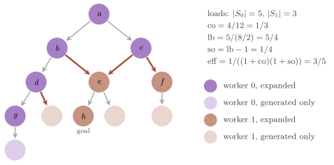
The estimates have measured counterparts in the SearchStats of a run
(§8.2): communication_overhead() is the
CO of Definition 8.2; load_balance() the
LB of Definition 8.3 on the expansions of
each worker; storage_balance() (Solution.h:121) the
same ratio on the nodes stored by each worker at the end (stored_by, the
states that it owns and has received), which is the LB of equation (3) of
[5], measured on all the states generated
rather than on those of \(f < C^*\); and search_overhead( sequential )
(Solution.h:134) the SO of
Definition 8.1, \(\mathrm{expanded} /
\mathrm{sequential} - 1\), given the expansions of a sequential run (and 0
if they are 0). The storage balance returns 1, as load_balance() does,
when the vector is empty or all 0
(src/Solution.cpp:62-79).
We remark on what the estimates do not see. They ignore the states of \(f \ge C^*\) that a parallel search expands because of the order of the expansions (the band and burst effects of section 3.1 of [5]), the re-expansions, the latency of the messages and the cost of the hash itself; and the model of Proposition 10.7 assumes that the imbalance of the states of \(f < C^*\) is the imbalance of the work, which holds only if the workers expand the other states at the same rate. A sample that is a prefix of the layer \(f < C^*\) measures the balance of the states nearest to the root, which may fall into fewer classes than those of the whole layer (cf. Corollary 10.13). The estimates are therefore a means of ranking distributions on an instance, not a prediction of its speedup.
10.4 The key as a linear map¶
All the distributions of this chapter are Zobrist hashing on some table, and Zobrist hashing is linear over the field GF(2) of two elements; this gives a single statement of what each of them keeps on the worker of the parent, and of what it costs in balance. We identify a set of features with its indicator vector in \(GF(2)^n\), so that \(x(s) \in GF(2)^n\) is the vector of \(F(s)\), the exclusive or of sets is the sum of vectors, and \(e_x\) is the vector of the single feature \(x\).
Definition 10.9 (The key matrix and the change vector). The key matrix of a table \(R\) is the \(32 \times n\) matrix \(H\) over GF(2) whose column \(x\) holds the high 32 bits of \(R[x]\). The change vector of a move from \(s\) to \(t\) is \(\delta = x(s) + x(t)\), i.e., the vector of \(F(s) \triangle F(t)\). For a subspace \(V\) of \(GF(2)^n\), a table vanishes on \(V\) if \(H v = 0\) for every \(v \in V\).
Theorem 10.10 (The moves that keep the key). Let \(H\) be the key matrix of a table. (i) The key of \(s\) is \(k(s) = H x(s)\), and a move with change vector \(\delta\) gives \(k(t) = k(s) + H \delta\); hence it keeps the key if and only if \(\delta \in \ker H\), and a move that keeps the key keeps the owner for every \(p\). (ii) For \(p = 2^b\), the owner of a key is its first \(b\) bits, and a move keeps the owner if and only if the first \(b\) rows of \(H\) vanish on \(\delta\).
Proof. (i) The key is the high 32 bits of \(\bigoplus_{x \in F(s)}
R[x]\), and taking the high bits commutes with \(\oplus\); hence \(k(s) =
\sum_{x \in F(s)} H e_x = H x(s)\), and by linearity \(k(t) = H(x(s) +
\delta) = k(s) + H \delta\). The owner is a function of the key. (ii)
key_owner( k , 2^b ) is \(\lfloor k \, 2^b / 2^{32} \rfloor\), i.e., \(k\)
shifted right by \(32 - b\) bits, which is its first \(b\) bits (the high
ones). Two keys have the same first \(b\) bits if and only if their sum
vanishes there, and \(k(s) + k(t) = H \delta\). \(\square\)
For other values of \(p\) the owners of two distinct keys may coincide, and a move outside \(\ker H\) keeps the owner with probability about \(1 / p\) (Corollary 10.13 below). Each distribution of this chapter is the choice of a subspace \(V\) on which its table vanishes, together with a table drawn among those that vanish on \(V\); the larger \(V\), the more moves keep their owner, but also the fewer distinct keys the states take. The following lemma, in which we take the free entries of the table independent and uniform (a model of the table drawn from the seed, as in Proposition 9.11), states what a table drawn uniformly among those that vanish on \(V\) does.
Lemma 10.11 (Uniform tables vanishing on a subspace). Let \(H\) be uniform among the \(32 \times n\) matrices that vanish on a subspace \(V\), and let \(V^\perp = \{r \in GF(2)^n : r \cdot v = 0 \text{ for all } v \in V\}\) be its annihilator. (i) The rows of \(H\) are independent and uniform on \(V^\perp\). (ii) For \(\delta \in V\), \(H \delta = 0\); for \(\delta \notin V\), \(H \delta\) is uniform on \(GF(2)^{32}\). (iii) For \(\delta, \delta'\) with \(\delta\), \(\delta'\) and \(\delta + \delta'\) outside \(V\), the pair \((H \delta, H \delta')\) is uniform on \(GF(2)^{64}\).
Proof. (i) \(H v = 0\) means that each row \(r\) of \(H\) has \(r \cdot v = 0\); hence the matrices that vanish on \(V\) are the matrices whose 32 rows lie in \(V^\perp\), a product of 32 copies of \(V^\perp\), and the uniform measure on a product is the product of the uniform measures. (ii) The first claim is the definition. If \(\delta \notin V\), then, since \((V^\perp)^\perp = V\) in a finite-dimensional space, some \(r \in V^\perp\) has \(r \cdot \delta = 1\); the map \(r \mapsto r \cdot \delta\) is then a nonzero linear form on \(V^\perp\), which takes each value on half of \(V^\perp\), so that each bit of \(H \delta\) is uniform, and the bits are independent by (i). (iii) The map \(r \mapsto (r \cdot \delta, r \cdot \delta')\) from \(V^\perp\) to \(GF(2)^2\) is linear; if it were not onto, its image would be annihilated by some nonzero \((\alpha, \beta)\), i.e., \(r \cdot (\alpha \delta + \beta \delta') = 0\) for all \(r \in V^\perp\), and \(\alpha \delta + \beta \delta' \in V\), which is one of \(\delta\), \(\delta'\), \(\delta + \delta'\). Hence it is onto, each pair of bits is uniform, and the 32 pairs are independent by (i). \(\square\)
Corollary 10.12 (The subspaces of Z and AZ).
(i) Zobrist hashing is the uniform table vanishing on \(V = \{0\}\). (ii) For
a projection \(A\), let
$\(V_A = \mathrm{span}\left(\{e_x + e_y : A(x) = A(y)\} \cup \{e_x : x
\text{ ignored}\}\right) ;\)$
then \(\delta \in V_A\) if and only if, for every abstract feature \(a\), an
even number of the features of \(\delta\) have \(A(x) = a\); and the table of
FeatureAbstraction::table() is uniform among the tables that vanish on
\(V_A\). Hence a move keeps the key with probability 1 if every abstract
feature appears an even number of times among its changed features, and
with probability \(2^{-32}\) otherwise.
Proof. (i) The entries of Zobrist hashing are independent and uniform, and every matrix vanishes on \(\{0\}\). (ii) A generator of \(V_A\) changes by 0 or 2 the number of its features in each abstract feature, or adds an ignored feature; hence the counts of a sum of generators are even. Conversely, a vector with even counts is, in each abstract feature, a set of an even number of features \(x_1, \ldots, x_{2m}\), the sum of the pairs \(e_{x_{2j-1}} + e_{x_{2j}}\), plus a set of ignored features, a sum of the \(e_x\). A matrix vanishes on \(V_A\) if and only if its columns are equal within each abstract feature and 0 at the ignored features; the table of the projection has the columns given by \(R'[A(x)]\) and 0, with \(R'\) uniform, and the map from \(R'\) to these matrices is a bijection, so that the table is uniform among them. The last claim is Lemma 10.11(ii). \(\square\)
This is the form of Corollary 9.13 for any projection. Figure 10.2 shows the key matrices of Z, of AZ and of a kernel table (§10.8) on six features.
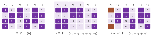
The price of a larger \(V\) is in the balance. The key of a state depends only on its class \(x(s) + V\), and the classes of the states of the sample are the units that the hash distributes.
Corollary 10.13 (The classes of a subspace). Let the table be uniform among those vanishing on \(V\), and partition the expanded states \(E\) of the sample into the classes \(C_1, \ldots, C_m\) of the relation \(x(s) + x(t) \in V\). (i) All the states of a class have one key, and therefore one owner. (ii) Two states of distinct classes, neither of which has \(x(s) \in V\), have independent uniform keys, and therefore the same owner with probability in \([1/p, 1/p + 2^{-32}]\). (iii) Whatever the table, \(\mathrm{lb} \ge p \max_j |C_j| / |E|\).
Proof. (i) By Theorem 10.10, \(k(s) + k(t) = H(x(s) + x(t)) = 0\). (ii) Lemma 10.11(iii) with \(\delta = x(s)\) and \(\delta' = x(t)\), whose sum is outside \(V\) since the classes differ; the bound on the probability is then the proof of Corollary 9.12. (iii) The worker that owns the largest class owns at least \(\max_j |C_j|\) states. \(\square\)
The corollary is the trade-off of the chapter in its exact form: the communication falls with the moves whose change vectors enter \(V\), and the balance is bounded by the largest class, whose size grows with \(V\); in the limit \(V = GF(2)^n\) every state has the key 0 and \(\mathrm{lb} = p\). Of course, a distribution need not be uniform among the tables that vanish on its \(V\) to keep the moves of \(V\); but all the constructions of the library are, as the following sections show, so that each of them is described by its subspace alone.
10.5 Cutting the transition graphs¶
GAZHDA\(^*\), GRAZHDA\(^*\) and FAZHDA\(^*\) cut the DTG of each group in two
sides \(S_1\) and \(S_2\), which become two abstract features of the group
(section 4.2.1 of [5] and section 6 there); for
\(G\) groups the states are partitioned into at most \(2^G\) classes, the
patterns of the sides of their features, which Abstract Zobrist hashing
maps to the workers. The projection is built by detail::cut_abstraction()
(AutoDistribution.h:700-727): the members
of a cut group get the abstract feature of their side, two new abstract
features per group; the features of an ignored group are ignored; and
every other feature (those of a group of fewer than two members, those
with no group, and those of a group that hold in no state of the sample
and that no transition changes) is its own abstract feature.
Proposition 10.14 (The moves that a cut
keeps). Let the projection \(A\) be a cut abstraction and a move change, in
each group, either nothing or one member \(x_g\) into another member \(y_g\)
(as a move of a FeatureGroupDomain with one feature per group does).
Then the move keeps the key with probability 1 if, in each changed group
that is cut and not ignored, \(x_g\) and \(y_g\) lie on the same side, and with
probability \(2^{-32}\) if some such group has them on two sides.
Proof. The changed features of a group \(g\) are \(x_g\) and \(y_g\). If \(g\) is ignored, both are; if \(g\) is cut, \(A(x_g) = A(y_g)\) exactly when they are on the same side, and the two abstract features of \(g\) appear in no other group. Hence every abstract feature appears an even number of times among the changed features if and only if no cut group has its two features on two sides, and the claim is Corollary 10.12(ii). \(\square\)
Hence the CO of a cut abstraction on the sample is, up to the factor of about \(1 - 1/p\) of Corollary 10.13(ii), the fraction of the moves that cross the cut of some group, i.e., the sampled weight of the edges cut in all the DTGs over the moves, if the moves change one group each; this is why the sampled weights measure the communication of a cut.
GAZHDA\(^*\): the greedy halves¶
greedy_abstraction() (AutoDistribution.h:943)
cuts each DTG by Algorithm 4 of [5], which
detail::greedy_cut() implements with the degrees and the links of the
static DTG (Algorithm 10.3); the degree of a node is the number of its
neighbours among the members, and its link the number of its neighbours
already in \(S_1\).
Algorithm 10.3 (GAZHDA\(^*\): the greedy halves of a DTG).
 1  function GREEDY-CUT(X)                    ▷ X the n members of the group
 2     if n < 2 then return (∅, X)
 3     deg(x) ← the static neighbours of x in X, for each x ∈ X
 4     link(x) ← 0 for each x ∈ X
 5     x₀ ← the node of least deg, of least index on ties
 6     S₁ ← {x₀}; link(y) ← link(y) + 1 for each static neighbour y of x₀
 7     while 2 |S₁| < n do
 8        x ← the node of X ∖ S₁ of largest link, of least index on ties
 9        S₁ ← S₁ ∪ {x}; link(y) ← link(y) + 1 for each static neighbour y of x
10     return (S₁, X ∖ S₁)
Lemma 10.15 (The greedy halves are balanced). For \(n \ge 2\), Algorithm 10.3 returns \(|S_1| = \lceil n / 2 \rceil\) and \(|S_2| = \lfloor n / 2 \rfloor\), i.e., \(|S_2| \le |S_1| \le |S_2| + 1\), whatever the edges, in \(O(n^2 + |E_X|)\) time for the static edges \(E_X\) of the DTG.
Proof. Each iteration of the loop adds one node, and the loop runs while \(2 |S_1| < n\), i.e., until \(|S_1| \ge n / 2\), the least such integer being \(\lceil n / 2 \rceil\). Each iteration scans the \(n\) nodes, and each node updates the links of its neighbours once, when it enters \(S_1\). \(\square\)
The cut is balanced in the number of members, not in the mass of the sample, and the paper notes (section 6.2.1 of [5]) that the balance is paid with the edges it cuts: on the logistics DTG of Figure 16 there, it cuts 21 edges where the sparsest cut cuts one. On the grid graph of a tile of the 15-puzzle the greedy side grows from the corner cell 0 along the rows and stops after the first two rows, which is the projection of a tile onto the half of the board of §9.4 (Exercise 10.4).
GRAZHDA\(^*\): the cut of largest sparsity or efficiency¶
sparsest_cut_abstraction()
(AutoDistribution.h:987) cuts each DTG at the
two sides of best objective, by detail::best_cut(). For a cut with side
masses \(m_1 = q(S_1)\) and \(m_2 = q(S_2)\) (of total \(M\)) and cut weight
\(\omega\) (of total \(W\)), the three objectives of CutObjective are:
sparsity: \(m_1 m_2 / \omega\) with the static weights, a node weighing 1 and an edge the ground operators that realize it, which is equation (6) of [5] for two parts (with the sizes as fractions and the weights normalized, a constant factor that changes no maximizer);sampled_sparsity: the same ratio with the weights of the sample, a node weighing its mass and an edge the moves that cross it, so that a cut weighs the part of the state space that the search visits rather than the domain of the variable;efficiency: \(1 / ((1 + c \, \omega / W) \max(m_1, m_2) / (M / 2))\) with the weights of the sample, the estimated efficiency of Definition 10.6 for this DTG alone and two workers.
A cut of weight 0 counts as a cut of weight \(10^{-9} W\), so that among the cuts that cut nothing the most balanced wins; if no member has a mass (a group seen only in generated states), the nodes weigh 1. The paper proposes the sparsity, finds the objective that minimizes \(\mathrm{CO} + \mathrm{LB}\) comparable to it, and leaves the others open (section 6.2 there); the two variants weighed by the sample are ours. The DTGs of up to 20 nodes are cut optimally by Algorithm 10.4, in which the node 0 stays on side 0 and the other nodes visit all their \(2^{n-1}\) assignments in the order of a Gray code.
Algorithm 10.4 (GRAZHDA\(^*\): the best cut of a DTG of at most 20 nodes).
 1  function BEST-CUT(X, q, w, value)   ▷ nodes 0, …, n − 1; q, w their weights
 2     side(x) ← 0 for each x; m₁ ← 0; ω ← 0
 3     best ← side; v* ← value(0, 0)
 4     for i ← 1 to 2^(n−1) − 1 do
 5        k ← 1 + (the number of the trailing zero bits of i)
 6        for each neighbour u of k do
 7           ω ← ω + w(k, u) if side(u) = side(k), ω − w(k, u) otherwise
 8        side(k) ← 1 − side(k)
 9        m₁ ← m₁ + q(k) if side(k) = 1, m₁ − q(k) otherwise
10        if value(m₁, ω) > v* then best ← side; v* ← value(m₁, ω)
11     return best
Lemma 10.16 (The enumeration is exact). For a DTG of \(n \ge 2\) nodes, Algorithm 10.4 evaluates every cut with node 0 on side 0 exactly once, the trivial cut (all the nodes on side 0) included, with its exact mass \(m_1\) and weight \(\omega\), and returns the first cut of largest value in the order of the enumeration; it takes \(O(2^{n-1} (\Delta + n))\) time for the largest degree \(\Delta\).
Proof. Let \(g(i) = i \oplus \lfloor i / 2 \rfloor\), the reflected Gray code of \(i\), read as the set of the nodes \(j + 1\) for the bits \(j\) of \(g(i)\), which are on side 1. Since \(g(i) \oplus g(i - 1) = (i \oplus (i - 1)) \oplus \lfloor (i \oplus (i - 1)) / 2 \rfloor\), and \(i \oplus (i - 1) = 2^{t + 1} - 1\) for the number \(t\) of the trailing zeros of \(i\), the two codes differ in the bit \(t\) only; hence the assignment after step \(i\) is \(g(i)\), by induction from \(g(0) = 0\). The map \(g\) is a bijection of \(\{0, \ldots, 2^{n-1} - 1\}\) (its inverse is the prefix exclusive or of the bits), so that the steps visit every nonzero assignment once, and line 3 the zero one. When \(k\) changes side, an edge \(\{k, u\}\) becomes cut if \(u\) was on the side of \(k\) and uncut otherwise, and no other edge changes, which is line 7; line 9 is the change of the mass of side 1. The strict comparison of line 10 keeps the first maximum. A step costs the degree of \(k\), and a new best cut a copy of \(n\) sides. \(\square\)
The header states the cost as \(O(2^n \bar{d})\) for the mean degree \(\bar{d}\); since the node \(k\) changes side \(2^{n-1-k}\) times, the cost of line 7 is \(\sum_k 2^{n-1-k} \deg(k)\), which is \(O(2^n \bar{d})\) on the regular grid graphs of the puzzles but is governed in general by the degrees of the low-numbered nodes, hence the bound with \(\Delta\). The paper cuts DTGs of fewer than 10 nodes by a depth-first branch-and-bound (section 6.2.3 of [5]) and suggests the algorithm of Fiduccia and Mattheyses [142] for the larger ones, which is what the library does above 20 nodes (Algorithm 10.5), from the greedy halves of Algorithm 10.3 and from the halves grown in breadth-first order from up to 16 nodes, the \(j\)-th from the node \(\lfloor j n / \min(n, 16) \rfloor\).
Algorithm 10.5 (GRAZHDA\(^*\): the passes of Fiduccia and Mattheyses from a cut \(s\)).
 1  function FM-PASSES(s)
 2     v ← value(s)
 3     repeat
 4        unlock every node; moved ← (); b ← v; l ← 0
 5        for step ← 1 to n do
 6           k ← the unlocked node whose move to the other side gives the largest value
 7           move k to the other side; lock k; append k to moved
 8           if value(s) > b · (1 + 10^−12) then b ← value(s); l ← |moved|
 9        move back the nodes moved after the l-th one
10        improved ← l > 0; if improved then v ← b
11     until not improved
12     return s
Proposition 10.17 (The passes). Algorithm
10.5 terminates, returns a cut whose value is at least that of \(s\), and
costs \(O(n (n + |E_X|))\) time per pass; the cut that best_cut() returns
is at least as good as each of its starts and as the trivial cut.
Proof. A pass ends with the cut after the best prefix of its moves
(line 9), whose value \(b\) is at least the value \(v\) at the start of the pass,
since \(\ell = 0\) restores the start. A pass is repeated only if
\(b > v (1 + 10^{-12})\), so that the values at the starts of the passes strictly
increase; as there are finitely many cuts, finitely many passes are made.
A step evaluates every unlocked node with the change of the cut weight at
that node, i.e., \(O(n + |E_X|)\) for the whole step, and a pass has \(n\)
steps. Finally, best_cut() starts from the trivial cut and keeps the
result of a start only if its value is larger. \(\square\)
No bound better than the finiteness of the cuts is known to us on the
number of passes, and the result is a local optimum, not the optimum. The
test distributions checks the enumeration against an independent
enumeration of the \(2^{15}\) cuts of three DTGs of the 15-puzzle with the
weights of the sample, and the passes on the 24-puzzle, whose DTGs have 25
nodes, by the cut of the paper: with the static weights GRAZHDA\(^*\) cuts
the 15-puzzle in two halves of two rows and the 24-puzzle in two rows
against three, the abstract features of Figure 19 of
[5] (Exercise 10.6). Figure 10.3
compares the two cuts on a tile of the 24-puzzle.
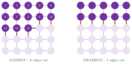
FAZHDA\(^*\): the fluent groups ignored¶
A group that nearly every move changes makes nearly every move change its
abstract feature, whatever the cut of the other groups (the hand of the
blocks world, Figure 12 of [5]);
fluency_abstraction()
(AutoDistribution.h:1010) ignores the
\(\lfloor \phi G \rfloor\) groups of largest fluency, for the fraction \(\phi\)
(0.3 by default, the best of 10% to 70% on the planning domains of section
5.2.1 of [5]), the ties going to the group of
least index, and cuts the others by Algorithm 10.3. By
Corollary 10.12, the subspace of FAZHDA\(^*\) contains \(e_x\) for
every feature of an ignored group, so that a move that changes only
ignored groups, or crosses no cut elsewhere, keeps its owner; by
Corollary 10.13 the classes grow by the combinations of the members of the
ignored groups that the sample holds. The paper notes (section 6.1) that
the fluency counts the changes of the features, whereas the owner changes
with the abstract features: a fluent group whose moves stay on one side of
its cut costs nothing, and ignoring it only coarsens the classes. On the
15-puzzle, with 15 groups and \(\phi = 0.3\), the 4 most fluent tiles are
ignored, as the test distributions checks.
10.6 State abstractions: AHDA\(^*\) and DAHDA\(^*\)¶
AHDA\(^*\) of Burns et al. [3] keeps the states with the same abstract state on one worker, the abstract state being, on a planning task, the values of a set \(P\) of variables chosen by the greedy abstraction of Zhou and Hansen [139] for structured duplicate detection. That algorithm adds one group at a time, the one that minimizes the locality
of the abstract graph \(S_P\) of \(P\) (equation (1) of
[139], self loops omitted), until the abstract
graph exceeds a bound \(N_{\max}\). The library computes \(\delta\) on the
abstract graph of the sample: the abstract state of a state for \(P\) is the
exclusive or of the words of its features in the groups of \(P\)
(words(), Definition 10.3), and an arc joins the abstract states of the
two ends of an edge of the sample that changes it. Algorithm 10.6 is
detail::zhou_hansen_groups()
(AutoDistribution.h:1049-1106).
Algorithm 10.6 (The greedy groups of Zhou and Hansen on the sample, with a stopping rule).
 1  function GREEDY-GROUPS(stop)
 2     P ← ∅; F ← 0; key(k) ← 0 for each state k of the sample
 3     loop
 4        for each group g ∉ P with members do
 5           cand(k) ← key(k) xor word(k, g) for each state k
 6           N(g) ← the distinct values cand(k)
 7           δ(g) ← (the most distinct cand(t) ≠ cand(s) over the edges (s, t) from one cand(s)) / |N(g)|
 8        if no group is left then break
 9        g* ← the group of least δ, then of least fluency, then of least index
10        if stop(F + |members(g*)|, |N(g*)|) then break
11        P ← P ∪ {g*}; F ← F + |members(g*)|
12        key(k) ← key(k) xor word(k, g*) for each state k
13        if F is the number of the members of all the groups then break
14     return P
state_abstraction() (AutoDistribution.h:1154)
stops before the group whose addition would give more than \(N_{\max}\)
abstract states on the sample (1000 by default), and
dynamic_state_abstraction()
(AutoDistribution.h:1125), DAHDA\(^*\) of
[138], stops before the group whose addition
would make the groups hold more than the fraction \(\rho\) of the members of
all the groups (0.3 by default, the best of 10%, 30%, 50% and 70% in
appendix A of [5]), but always keeps the first
group; both ignore the features of the groups not chosen, and keep every
other feature by itself.
Lemma 10.18 (The state abstractions). Let \(P\) be the groups chosen. (i) The key of a state depends only on its features in the groups of \(P\) and on its features without a group, and the subspace of the table contains \(e_x\) for every feature of a group outside \(P\). (ii) For DAHDA\(^*\), \(P\) is not empty if some group has members, and the members of \(P\) are at most \(\rho\) times those of all the groups unless \(P\) is the first group alone. (iii) For AHDA\(^*\), the states of the sample take at most \(N_{\max}\) abstract states for \(P\); in particular, if the first group chosen exceeds \(N_{\max}\) alone, \(P\) is empty and every state of the sample has the same key. (iv) Each round costs \(O(G (N + |M|))\) expected time for \(G\) groups, \(N\) states and \(|M|\) edges of the sample, and there are at most \(G\) rounds.
Proof. (i) The projection maps the features of the groups outside \(P\)
to no_abstract_feature, i.e., to the entry 0, and the others to their
own abstract features; Corollary 10.12 gives the subspace. (ii) The rule
of DAHDA\(^*\) returns false at its first call and then true exactly when
the members of the union would exceed \(\rho\) times the total. (iii) The
rule of AHDA\(^*\) stops before any addition that would give more than
\(N_{\max}\) values of the abstract key on the states of the sample, which
are its abstract states (the words of distinct sets of features being
distinct, with probability 1 in the model of random words); if the first
candidate exceeds the bound, nothing is added, and the features that
remain are those that no move changes, which are the same in every state
of the sample, since each state of the sample is reached from the root by
moves. (iv) A candidate costs a pass over the states and one over the
edges, with hash sets of the abstract states and of the arcs. \(\square\)
Thus the distribution of AHDA\(^*\) is Zobrist hashing of the abstract state
of \(P\), i.e., HDA\(^*\)[Z, Astate/SDD] of section 2.5 of
[5], with the abstract graph of the sample in
place of the abstract graph of the task. The difference between the two
rules is the one of [138]: a fixed bound on the
abstract states balances the load badly on instances of varying size (with
the bound of \(10^4\), AHDA\(^*\) ran out of memory on Blocks10-2 and Gripper8
on 48 cores, section 5 there), while a fraction of the features scales with
the instance. The ties of line 9 go to the group of least fluency, which
the papers do not specify; the abstraction of the nblocks of the planning
tasks breaks them by the larger graph instead
(Chapter 16). The test distributions checks that
DAHDA\(^*\) keeps at most 30% of the features of the 15-puzzle and that one
more tile would exceed the bound, and that AHDA\(^*\) with \(N_{\max} = 200\)
gives the states of the sample between 2 and 200 abstract states.
10.7 Operator-based Zobrist hashing: OZHDA\(^*\)¶
Instead of projecting the features, OZHDA\(^*\) (section 4 of
[138] and section 2.4 of
[5]) changes the table of Zobrist hashing so
that the hash of an operator, the exclusive or of the entries of the
features that it adds and deletes, is 0; a move by such an operator then
keeps the hash of its parent. operator_table()
(AutoDistribution.h:1191-1226) is
Algorithm 10.7.
Algorithm 10.7 (OZHDA\(^*\): the operator-based table).
 1  function OPERATOR-TABLE(φ, paper)
 2     R ← the table of Zobrist hashing drawn from the seed
 3     ops ← the operators of the sample, by decreasing weight
 4     if paper then sort ops stably by increasing number of features
 5     mask ← all the 64 bits if paper, the high 32 bits otherwise
 6     for each of the first ceil(φ · |ops|) operators a of ops do
 7        if a has fewer than 2 features then continue
 8        x ← the first feature of a, by index, that is not fixed
 9        if there is none then continue
10        set the bits of mask of R[x] to the xor of those of R[y], y ∈ a ∖ {x}
11        fix every feature of a
12     return R
Proposition 10.19 (The operators that OZHDA\(^*\) keeps). Call an operator fixing if it reaches line 10, and let \(x_a\) be the feature that it sets. (i) For every fixing operator \(a\), the bits of mask of \(\bigoplus_{y \in a} R[y]\) are 0 in the returned table; hence a move by \(a\) keeps its key, and its owner, for every \(p\). (ii) The change vectors \(\delta_a\) of the fixing operators are linearly independent, and the returned key matrix is uniform among those vanishing on their span \(V_O\); hence, by Lemma 10.11, a move whose change vector is outside \(V_O\) keeps its key with probability \(2^{-32}\).
Proof. (i) Right after line 10 the masked bits of \(R[x_a]\) are the sum of those of the other features of \(a\), so that the masked bits of the sum over \(a\) vanish. An entry is changed only at line 10, and only for a feature that is not fixed; since line 11 fixes every feature of \(a\), no entry of a feature of \(a\) changes afterwards, and the sum stays 0. (ii) Order the fixing operators as they are processed. An operator \(a\) cannot contain \(x_b\) for a fixing \(b\) processed after it, since every feature of \(a\) is fixed after \(a\) whereas \(x_b\) is not fixed when \(b\) is processed; hence \(x_a\) is in \(\delta_a\) and in no earlier \(\delta_b\) (it was not fixed before \(a\)), and the vectors are independent, since in a vanishing sum the latest operator would be the only one with its feature \(x_a\). The key matrix has random columns at the features that no fixing operator sets, and at each \(x_a\) the sum of the columns of the other features of \(a\), which are features set earlier or never set; this is a bijection from the free columns onto the matrices that vanish on \(V_O\) (in such a matrix the column \(x_a\) is determined by the others, by induction on the order), so that the key matrix is uniform among them. \(\square\)
The paper processes all the actions, by increasing number of
preconditions, and sets the whole entry; the library processes the
operators of the sample by decreasing weight up to the fraction \(\phi\)
(0.2 by default) and sets only the 32 bits of the key, and with
as_paper (the name OZP, all the operators by default) it sets the whole
entry and orders the operators by increasing number of changed features,
which stands for the number of preconditions that a FeatureDomain does
not give, the ties keeping the order of frequency. An operator whose
features are all fixed is skipped (line 9) even if its change vector is
outside \(V_O\), which Algorithm 10.7 cannot see; KZHDA\(^*\)
(§10.8) tests membership in the subspace instead. Since each
fixing operator joins its new feature to features already joined, the
operators of a DTG join whole paths of it into one class: on a tile of a
puzzle the operators are the edges of its grid, and a large fraction of
them makes most of the cells of a tile one class, which by
Corollary 10.13 balances the load badly (the paper's
criticism of the bottom-up clustering of OZHDA\(^*\), section 6.1 of
[5]). The test distributions checks (i) on
the most frequent operator of a sample of the 15-puzzle, and that the
estimated CO of OZHDA\(^*\) is below that of Zobrist hashing for \(p = 8\).
10.8 Kernel selection: KZHDA\(^*\)¶
By Theorem 10.10 and Corollaries 10.12 and 10.13, a distribution is, up to the draw of its table, the subspace \(V\) on which its key vanishes: Z is \(V = \{0\}\), AZ is \(V_A\), the cuts of the DTGs and the state abstractions are particular projections, and OZHDA\(^*\) is \(V_O\). KZHDA\(^*\) chooses \(V\) directly: the change vectors of the most frequent operators of the sample are inserted into a basis of \(V\) by Gaussian elimination over GF(2), an operator being kept if the table of the larger subspace has a larger estimated value, and the table is drawn uniformly among those that vanish on \(V\). This construction is ours; its starting point is the observation of section 6.1 of [5] that all the earlier distributions are clusterings followed by a partition of the DTGs.
The basis¶
Gf2Basis (AutoDistribution.h:1237-1295)
keeps a basis of a subspace of \(GF(2)^n\) as rows of 64-bit words, each with
a pivot:
class Gf2Basis {
 public:
 using Vector = std::vector< std::uint64_t >;
 explicit Gf2Basis( std::size_t n );
 std::size_t rank( void ) const noexcept;
 bool insert( const std::vector< std::uint32_t > & bits );
 std::pair< std::vector< Vector > , std::vector< std::uint32_t > >
  reduced( void ) const;
 };
Algorithm 10.8 (The basis over GF(2): the rows ρ(1), …, ρ(r) with the pivots π(1), …, π(r)).
 1  function INSERT(v)                       ▷ v the vector of the given bits
 2     for j ← 1 to r do
 3        if v has the bit π(j) then v ← v xor ρ(j)
 4     if v = 0 then return false
 5     r ← r + 1; ρ(r) ← v; π(r) ← the least bit of v
 6     return true
 7  function REDUCED()                        ▷ on a copy of the rows
 8     for j ← r down to 1 do
 9        for q ← j + 1 to r do
10           if ρ(j) has the bit π(q) then ρ(j) ← ρ(j) xor ρ(q)
11     return the rows and the pivots
Lemma 10.20 (The echelon form). (i) After each
insertion, every row \(\rho(j)\) has the bit \(\pi(j)\) and none of the bits
\(\pi(q)\), \(q < j\); the rows are independent and span the subspace spanned
by the vectors inserted. (ii) insert( v ) returns true if and only if
\(v\) is not in the span of the earlier vectors, i.e., the rank grows. (iii)
reduced() returns rows that span the same subspace, each with the bit of
its own pivot and none of the pivots of the other rows (reduced row
echelon form, up to the order of the rows). An insertion costs \(O(r n /
64)\) and the reduction \(O(r^2 n / 64)\).
Proof. (i) and (ii), by induction on the insertions. At step \(j\) of lines 2 and 3, \(v\) loses the bit \(\pi(j)\) if it had it; a later step \(q > j\) adds \(\rho(q)\), which by induction lacks \(\pi(j)\), so that the bit stays at 0. Hence the final \(v\) lacks every pivot; if it is not 0, its least bit is a new pivot, and the new row satisfies (i). The vector given is the final \(v\) plus a sum of rows, so that the span grows by it exactly when \(v \ne 0\), which is (ii). The rows are independent: in a vanishing sum of rows, the row of least index \(j\) in it is the only one with the bit \(\pi(j)\), since the rows after it lack it. (iii) We show, for \(j\) from \(r\) down to 1, that after its loop the row \(j\) has its own pivot and no other one, and that every row keeps the property of (i). The rows \(q > j\) already have only their own pivots; adding \(\rho(q)\) to \(\rho(j)\) clears the bit \(\pi(q)\) and changes no other pivot bit, so that after the loop \(\rho(j)\) has no \(\pi(q)\), \(q > j\), still none of the \(\pi(q)\), \(q < j\) (the rows added lack them), and still \(\pi(j)\) (the rows \(q > j\) lack it). Row operations keep the span. The costs are those of the loops on vectors of \(\lceil n / 64 \rceil\) words. \(\square\)
The kernel table¶
kernel_table() (AutoDistribution.h:1310-1326)
draws the table of Zobrist hashing from the seed and overwrites the high
32 bits of the entry of each pivot.
Algorithm 10.9 (The kernel table of a basis \(B\)).
 1  function KERNEL-TABLE(n, B)
 2     R ← the table of Zobrist hashing on n features, drawn from the seed
 3     (ρ, π) ← REDUCED() of B
 4     for j ← 1 to r do
 5        y ← the xor of the high 32 bits of R[x], for x ∈ ρ(j), x ≠ π(j)
 6        replace the high 32 bits of R[π(j)] by y
 7     return R
Theorem 10.21 (The kernel table). Let \(V\) be the span of \(B\). (i) The table vanishes on \(V\); hence every move whose change vector is in \(V\) keeps its key and its owner. (ii) If the entries drawn from the seed are independent and uniform, the key matrix is uniform among the matrices that vanish on \(V\), and its rows are independent and uniform in \(V^\perp\); hence a move whose change vector is outside \(V\) keeps its key with probability \(2^{-32}\), and the owners of the classes of \(V\) are those of Corollary 10.13. (iii) The low 32 bits of every entry, and the high bits of every non-pivot feature, are those of Zobrist hashing with the same seed.
Proof. (i) By Lemma 10.20(iii) the features of \(\rho(j)\) other than \(\pi(j)\) are not pivots, so that their entries are not changed by line 6, for any \(j\); hence after line 6 the high bits of \(\bigoplus_{x \in \rho(j)} R[x]\) are \(y \oplus y = 0\), i.e., \(H \rho(j) = 0\), and by linearity \(H\) vanishes on the span of the rows, which is \(V\). Theorem 10.10 gives the moves. (ii) A matrix that vanishes on \(V\) has, at each pivot \(\pi(j)\), the column equal to the sum of the columns of the other features of \(\rho(j)\), all non-pivots; conversely any choice of the non-pivot columns gives, by lines 4 to 6, a matrix that vanishes on \(V\). Hence the map from the non-pivot columns to the result is a bijection onto the matrices that vanish on \(V\), and uniform non-pivot columns give a uniform matrix; Lemma 10.11 and Corollary 10.13 apply. (iii) Line 6 changes only the high bits of the pivots. \(\square\)
The test distributions checks (i) on a basis of 8 features with a
dependent vector (Exercise 10.10), and on the subspace of the 40 most
frequent operators of a sample of the 15-puzzle.
The selection of the subspace¶
kernel_selection_table()
(AutoDistribution.h:1362-1402) grows \(V\)
greedily over the candidate operators of largest weight (1024 by default),
by decreasing weight, from \(\{0\}\) or from the subspace \(V_A\) of a
projection \(A\) given by the caller (Algorithm 10.10). The value of a table
is the smaller of its estimated efficiencies among \(p\) and among \(2p\)
workers (estimate_table()): the sample holds the states of least \(f\),
which A\(^*\) expands first, and a subspace that balances them among \(p\)
workers only through a few classes balances the later states badly,
which the estimate among \(2p\) workers exposes. The table of every
subspace is drawn from the same seed, so that two steps differ only in
the entries of the pivots, and an operator already in \(V\) costs nothing.
Algorithm 10.10 (KZHDA\(^*\): the selection of the kernel).
 1  function KERNEL-SELECTION(p, c, K, A)
 2     B ← the basis of {0}
 3     if a projection A is given then
 4        for each feature x, by index, do
 5           if A ignores x then INSERT(e_x) into B
 6           else if some y < x has A(y) = A(x) then INSERT(e_y + e_x) into B, y the last one
 7     T ← KERNEL-TABLE(n, B); v ← min(eff(T, p), eff(T, 2p))
 8     for each of the first K operators a, by decreasing weight, do
 9        B' ← a copy of B
10        if not INSERT(δ_a) into B' then continue        ▷ already in the span
11        T' ← KERNEL-TABLE(n, B')
12        if min(eff(T', p), eff(T', 2p)) > v then B ← B'; T ← T'; v ← that value
13     return T
Proposition 10.22 (The selection). (i) The vectors inserted at lines 4 to 6 span \(V_A\), so that the start is a table uniform among those that vanish on \(V_A\), i.e., Abstract Zobrist hashing with \(A\) in law (not entry by entry). (ii) The returned table vanishes on the span of the start and of the accepted operators, so that every move by an accepted operator keeps its owner. (iii) Its value \(\min(\mathrm{eff}(T, p), \mathrm{eff}(T, 2p))\) is at least that of the start, and so is its estimated efficiency among \(p\) workers, i.e., \(\mathrm{eff}(T, p)\) is at least the value of the start. (iv) A step costs \(O(r^2 n / 64 + n + N_F)\) time, for the rank \(r\) and the number \(N_F\) of the features of all the states of the sample.
Proof. (i) In each abstract feature, the vectors \(e_y + e_x\) of consecutive members form a path, whose sums are the even subsets of the class, and the \(e_x\) of the ignored features span the rest; this is the set of Corollary 10.12(ii). Theorem 10.21(ii) gives the law. (ii) Theorem 10.21(i) for the final basis, which contains the start and the accepted vectors. (iii) \(v\) only increases at line 12, and the returned table is the one of the last increase, or the start; and \(\mathrm{eff}(T, p) \ge \min(\mathrm{eff}(T, p), \mathrm{eff}(T, 2p)) = v \ge v_0\). (iv) A copy and an insertion cost \(O(r n / 64)\), the reduction \(O(r^2 n / 64)\), the table \(O(n)\), and two estimates read the features of the states of the sample. \(\square\)
We remark that (iii) does not say that the estimated efficiency of the
result among \(p\) workers is at least that of the start among \(p\) workers:
the start may be better among \(p\) workers and worse among \(2p\). The test
distributions compares the efficiency of KZHDA\(^*\) among 8 workers with
that of Zobrist hashing among 8 workers, which holds on its instance but
does not follow from the code (Exercise 10.11). The names KZ:GRAZ,
KZ:GRAZS, KZ:GRAZE and KZ:DAHDA start from the subspace of that
projection, built on the same model; with KZ the start is Zobrist
hashing. With \(p\) a power of 2, Theorem 10.10(ii) shows that a table need
only vanish with its first \(b\) rows to keep the owners; the library makes
all 32 rows vanish, so that the key, and not only the owner, is kept, and
the moves that keep their owner are the same for every \(p\).
10.9 The automatic choice¶
auto_distribution() (AutoDistribution.h:1522-1545)
builds every distribution of auto_distribution_names()
(AutoDistribution.h:1409), the methods of this
chapter with their parameters at a few values around the default,
Z  GAZ  GRAZ  GRAZS  GRAZE  FAZ:0.1  FAZ:0.3  FAZ:0.5  OZ:0.1  OZ:0.2  OZ:0.3
DAHDA:0.2  DAHDA:0.3  DAHDA:0.5  AHDA:100  AHDA:1000  AHDA:10000
KZ  KZ:GRAZS  KZ:GRAZE  KZ:DAHDA
(21 names; OZP and KZ:GRAZ are accepted by make_distribution() but
are not among them), adds the distributions of extra, estimates each one
on the sample among \(p\) workers with the cost \(c\), and returns the one of
largest estimated efficiency.
Algorithm 10.11 (The automatic choice).
 1  function AUTO-DISTRIBUTION(m, p, c, extra)
 2     C ← MAKE-DISTRIBUTION(m, name, c, seed, p) for each name, then extra
 3     best ← the first X ∈ C of largest eff of ESTIMATE(X, p, c)
 4     if est is given then est ← the estimate of best
 5     return the table distribution of the table of best, named "auto:" and its name
Proposition 10.23 (The automatic choice). The
returned distribution has the table of a candidate of largest estimated
efficiency among \(p\) workers, the first in the order of the names and then
of extra on ties, and therefore the owners of that candidate; HDA\(^*\)
with it returns an optimal path (Proposition 10.1). The construction draws
nothing but the table from the seed, so that two processes that build it
on the same instance, with the same parameters and the same order of the
successors, obtain the same table.
Proof. Line 3 keeps the first candidate of strictly largest efficiency. The returned distribution is built from the table of that candidate, and the owner is a function of the table (Proposition 10.1(i)). The sample is A\(^*\) with a deterministic OPEN list; the maps that the constructions iterate are ordered, the hash tables are only searched or counted, and every tie is broken by index or by order, so that the result depends on the instance, the parameters and the seed only. \(\square\)
The choice rests on the correlation of the estimated with the actual
efficiency found in section 5.2.1 of [5]; beyond
the choice of the method, it tunes the fractions of FAZHDA\(^*\), OZHDA\(^*\)
and DAHDA\(^*\) and the bound of AHDA\(^*\), which the papers fix once for all
the instances. Its cost is that of building the 21 candidates and of 21
estimates, of which the 4 kernel selections, each of up to 1024 steps of
Proposition 10.22(iv), are by that bound the most expensive. The test
distributions checks that the chosen name begins with auto: and that
no candidate has a larger estimate, and solves logistics-4-0 with the
automatic distribution on 1 and 3 workers; on blocks-6-2 it solves the
task with every candidate.
The hand-made projections of the sliding-tile puzzles¶
The projections of the sliding-tile puzzles compared by Jinnai and
Fukunaga (footnote 4 of section 3.1.4, footnote 6 of section 3.2 and
Figure 8 of [5], and
[141]) are
given by SlidingTile::tile_abstraction()
(SlidingTile.h:493-515), which returns, for a
TileRegions and a list of tiles, the table of a FeatureAbstraction:
enum class TileRegions { single , pair , line , block , half , quad , cross ,
                         odd };
[[nodiscard]] static std::vector< std::uint32_t > tile_abstraction(
 TileRegions r , const std::vector< int > & tiles = {} );
The abstract feature of "tile \(t\) in cell \(c\)" is the pair of \(t\) and of
the region of \(c\) for the tiles of the list (all if it is empty), and the
other tiles are ignored; the regions are the following
(SlidingTile.h:844-875).
TileRegions |
The regions of the cells of a board of \(W \times H\) cells |
|---|---|
single |
each cell by itself, i.e., Zobrist hashing |
pair |
the cells \(2k\) and \(2k + 1\), in the order of the rows |
line |
the rows |
block |
the blocks of \(2 \times 2\) cells (smaller on the last row or column of an odd board) |
half |
the first \(\lfloor W H / 2 \rfloor\) cells and the others |
quad |
four blocks of 6 cells, the center ignored (\(5 \times 5\) only) |
cross |
five regions of 5 cells around the center (\(5 \times 5\) only) |
odd |
the middle column and four regions of 5 cells (\(5 \times 5\) only) |
Ignoring all the tiles but a few gives the AHDA\(^*\) of Burns et al. as
Zobrist hashing of the abstract state (e.g., the tiles 1 to 3 on the
15-puzzle, the abstraction chosen for AHDA\(^*\) in footnote 4 of
[5]). A region that the board has not, or a
tile outside \([1, W H)\), throws std::invalid_argument. These projections
can be passed to auto_distribution() in extra, as
TableZobristDistribution< D >( d , FeatureAbstraction::of( D::tile_abstraction( r ) ) , seed , name ),
so that the automatic choice compares them with the constructions. The
test distributions counts the regions of each projection on the
15-puzzle and on the 24-puzzle, and solves two instances of the 24-puzzle
with HDA\(^*\) on 2 workers under every construction and under the
projections quad, cross, odd, line and half on the tiles 1 to 5.
The benchmark tool¶
The option --dist of tools/AStarBench.cpp takes, besides
the distributions of Chapter 9 (Z, AZ, A,
P, H, R) and the hyperplanes (HWD, Chapter 15),
every name of make_distribution(), AUTO for auto_distribution() (whose
choice is printed in the column chosen), and tile:<regions>[:<tiles>] for
a hand-made projection, e.g., tile:block:1-4; --sample sets the
expansions of the sample (32768) and --cost the cost \(c\) of a message (1).
The constructions are offered on the domains that are an
AbstractFeatureDomain or a FeatureGroupDomain (the puzzles, the grids and
the planning tasks), and run on the C++ threads or over MPI
(tools/AStarBenchSolve.h:473-553). Each run
prints the estimates of its distribution on the sample (the columns estCO,
estLB, sparsity and effesti) next to the measured CO, LB and
LBstored (the storage balance), and, with --so 1, the search overhead
SO against a run of A\(^*\) on the same instance; with --estimate 1 the
distributions of Chapter 9 are estimated as
well.
10.10 The engineering of the implementation¶
- The constructions read only a
FeatureGraph, which holds no state of theDomain: the features of each state are stored in one array with offsets (state_features()), and the words of the states in the groups in one array of \(N G\) words. Hence the constructions, the estimates of a table and the kernel selection are compiled once, and only the sample andFeatureModel::estimate()are instantiated perDomain. - The sample keeps each state in a hash map indexed by the hash of the
Domain, its values in parallel arrays, and the entries of OPEN as triples in a binary heap; the states are copied once more into the final order, the expanded ones first, so that the loads of an estimate are the firstnum_expanded()owners. - The operators are counted in an ordered map from their change sets, and the DTG edges in ordered maps from their pairs, which makes the construction deterministic (Proposition 10.23) at the price of a logarithmic factor per move.
estimate_table()computes the hash of each state from its stored features, i.e., in \(N_F\) lookups, which is what makes the two estimates of each step of the kernel selection affordable; the estimate of a distribution that is not a table calls itsowner()on the stored states.- The cuts use the static weights for the greedy halves and for the sparsity of the paper, and the sampled weights otherwise, both kept per feature as adjacency lists sorted by neighbour; the enumeration of the cuts reads the adjacency of the node that changes side only.
- The kernel table is recomputed from the seed at each step instead of being updated, which keeps every step independent of the rejected operators (Theorem 10.21(iii)).
10.11 Benchmark¶
Table 10.1. The distributions of this chapter and of Chapter 9, and the hand-made projections, on the 24-puzzle: estimated and measured overheads, and the speedup of HDA\(^*\) on the threads.
| distribution | estCO | estLB | effesti | CO | LB | LBstored | SO | seconds (speedup), 8 cores | seconds (speedup), 32 cores |
|---|---|---|---|---|---|---|---|---|---|
Placeholder: the results of this table are to be measured on an idle machine and written here by manual/build/tables.py; no number is given until then.
Table 10.2. The distributions of this chapter and of
Chapter 9 on the planning tasks of
data/planning.
| distribution | estCO | estLB | effesti | CO | LB | LBstored | SO | seconds (speedup), 8 cores | seconds (speedup), 32 cores |
|---|---|---|---|---|---|---|---|---|---|
Placeholder: the results of this table are to be measured on an idle machine and written here by manual/build/tables.py; no number is given until then.
The experiment runs HDA\(^*\) on the C++ threads with each distribution, on
the instances of the 24-puzzle distributed with the code of Jinnai and
Fukunaga (Table 10.1) and on the largest planning tasks of the tester
(Table 10.2), with batches of 64 nodes and flushes every 64 expansions,
on 8 and 32 cores, with samples of 32768 expansions and \(c = 1\). A row is
a distribution, by its name in --dist (for AUTO, the constructions
chosen on the instances are listed in the note under the table), and a
column gives, for a number of cores, the estimates on the sample
(\(\mathrm{co}\), \(\mathrm{lb}\) and \(\mathrm{eff}\)), the measured CO, LB and
storage balance, the search overhead against A\(^*\), and the time summed
over the instances with the speedup over A\(^*\) in parentheses. The time of
solve() is measured as in §9.8; the
time of the sample and of the construction of the distribution, which it
does not include, is given in a separate column, since it is the price
that an automatic distribution pays over a hand-made one. We remark that
the tables are placeholders until the campaign is run on an idle machine.
10.12 Notes and references¶
Abstract Zobrist hashing, and the greedy cut of the DTGs (GAZHDA\(^*\)), are from Jinnai and Fukunaga [141]; the fluency filter (FAZHDA\(^*\)), the operator-based Zobrist hashing (OZHDA\(^*\)) and the dynamic threshold of AHDA\(^*\) (DAHDA\(^*\)) from [138]; and the workload graph, the estimates of equations (3) to (5), the sparsity of equation (6), GRAZHDA\(^*\) and the reading of the earlier methods as clusterings followed by a partition of the DTGs from the journal paper [5], which also gathers the experiments of the two conference papers (on planning with the merge-and-shrink heuristic [140], on a cluster and on 128 virtual cores, and on the 24-puzzle). AHDA\(^*\) is from Burns et al. [3], who took the greedy abstraction of Zhou and Hansen [139] for structured duplicate detection; the DTG is that of SAS+ [133], as the planner Fast Downward [134] computes it; and the local search of the cuts is that of Fiduccia and Mattheyses [142]. In section 6.2.2 of [5] the correlation between the sparsity and the estimated efficiency is shown on partitions of the workload graph made by a graph partitioning package, which the library does not use.
The following facts are stated from the code and the papers, not from
measurements. The papers implement these distributions in Fast Downward,
for planning tasks, with the DTGs of the task and with the workload graph
computed by a full run of A\(^*\); the library builds them on a bounded
sample of any FeatureDomain, for which the DTGs, the operators and the
fluency are those of the moves of the sample, and the groups may be
inferred. The weights of the sample in the cuts, the objective of
efficiency, KZHDA\(^*\) and the choice by the estimate among all the
constructions are ours, and we have no measurement of them yet
(§10.11). The reading of every distribution as a subspace of
the kernel of a linear map (§10.4) makes precise the remark of
section 6.1 of [5] that all the earlier methods
are instances of GRAZHDA\(^*\) with a clustering; we are not aware of a
statement of it in this form. Finally, the hyperplane work distribution of
Kobayashi et al. [43] for the multiple
sequence alignment, which uses the levels of the alignment rather than its
features, is treated in Chapter 15.
10.13 Exercises¶
Exercise 10.1 (ctest -R PBeFS.distributions). Using
Proposition 10.1(iii), show that make_distribution( m , "Z" )
assigns every state to the same owner as ZobristDistribution with the
same seed, and say what would change if the generator drew the table
backwards; the test checks the owners of the states of a sample of the
15-puzzle for \(p = 7\).
Exercise 10.2 (ctest -R PBeFS.distributions). Prove that the DTG of
every tile of the 15-puzzle in a FeatureModel is its grid graph, i.e.,
that every edge joins two cells at Manhattan distance 1, and that the
groups inferred without num_feature_groups() are the tiles
(Lemma 10.5). Would the inference still give the tiles if the
puzzle listed no ground transitions and the sample were small?
Exercise 10.3 (ctest -R PBeFS.distributions). Show that for \(p = 1\)
the estimates of every distribution are \(\mathrm{co} = 0\) and
\(\mathrm{lb} = 1\), and explain by
Corollary 9.12 why the estimated CO of
Zobrist hashing among 8 workers exceeds 0.8 on a sample of the 15-puzzle.
Why is it not exactly \(7/8\)?
Exercise 10.4 (ctest -R PBeFS.distributions). Run Algorithm 10.3 by
hand on the grid graph of a tile of the 15-puzzle and show that it adds
the cells \(0, 1, \ldots, 7\) in this order, so that GAZHDA\(^*\) is there the
projection onto the halves of the board of
§9.4; then run it on the \(5 \times 5\)
grid and check the cut of Figure 10.3. The test checks that
each cut has two sides whose sizes differ by at most one
(Lemma 10.15).
Exercise 10.5 (ctest -R PBeFS.distributions). Prove that the
enumeration of Algorithm 10.4 is exact (Lemma 10.16) by
writing out its seven steps for \(n = 4\), with the side of each node and
the weight of the cut. The test compares the cut of GRAZHDA\(^*\) with the
weights of the sample against all the \(2^{15}\) cuts of three DTGs of the
15-puzzle.
Exercise 10.6 (ctest -R PBeFS.distributions). With the static
weights, show that the sparsest cut of the \(4 \times 4\) grid is two rows
against two and that of the \(5 \times 5\) grid two rows against three
(hint: a cut of \(k\) edges that does not cross the board from side to side
isolates a corner of at most \(k^2 / 4\) cells, and one that crosses it cuts
at least \(w\) edges of the \(w \times w\) grid). The test checks both cuts,
the second one found by the passes of Algorithm 10.5.
Exercise 10.7 (ctest -R PBeFS.distributions). Show that
fluency_abstraction( m , 0.3 ) ignores exactly 4 of the 15 groups of the
15-puzzle, those of largest fluency, and describe by
Corollary 10.13 how the classes of the states grow when one
more tile is ignored.
Exercise 10.8 (ctest -R PBeFS.distributions). Show that DAHDA\(^*\)
with \(\rho = 0.3\) keeps on the 15-puzzle at most 4 tiles, i.e., 64 of the
240 members of the 15 groups, and that a fifth tile would exceed the
bound; then find the conditions under which AHDA\(^*\) with \(N_{\max} = 200\)
keeps no group at all (Lemma 10.18(iii)), and what HDA\(^*\)
does with that distribution.
Exercise 10.9 (ctest -R PBeFS.distributions). Prove
Proposition 10.19(i) for the most frequent operator of a
sample of the 15-puzzle, and give an operator of the 15-puzzle that
Algorithm 10.7 may skip although its change vector is not in \(V_O\). Why
does a fraction close to 1 give a poor load balance?
Exercise 10.10 (ctest -R PBeFS.distributions). Insert the vectors
\(\{0, 1\}\), \(\{1, 2\}\), \(\{0, 2\}\) and \(\{5\}\) into a Gf2Basis of 8
features by Algorithm 10.8, and show that the third insertion returns
false and the rank is 3. Compute the reduced rows and the high bits of the
entries 0, 1, 2 and 5 of the kernel table, and the probability that the
high bits of the entry 3 are 0 (Theorem 10.21).
Exercise 10.11 (discussion, no test). Build a sample and two tables
\(T_0\) and \(T_1\) such that \(\min(\mathrm{eff}(T_1, p), \mathrm{eff}(T_1, 2p)) >
\min(\mathrm{eff}(T_0, p), \mathrm{eff}(T_0, 2p))\) but \(\mathrm{eff}(T_1,
p) < \mathrm{eff}(T_0, p)\), and conclude which part of the check of
KZHDA\(^*\) in the test distributions is guaranteed by
Proposition 10.22(iii) and which is not.
Exercise 10.12 (ctest -R PBeFS.distributions). Show that
auto_distribution() returns the table of a candidate of largest
estimated efficiency (Proposition 10.23), and that HDA\(^*\)
with it, or with any construction, returns an optimal plan on a planning
task (Proposition 10.1); the test solves blocks-6-2 with every candidate
and logistics-4-0 with the automatic choice, on 1 and 3 workers.
Exercise 10.13 (ctest -R PBeFS.hda-owners). Using
Theorem 10.10(ii), show that for \(p = 64\) the owner of a key
is its first 6 bits, that each owner has \(2^{26}\) keys, and that a move
keeps its owner among 64 workers if and only if the first 6 rows of the
key matrix vanish on its change vector; the test checks the owners of the
keys for \(p = 64\) among other values (cf.
Exercise 9.13).
Exercise 10.14 (discussion, no test). Write the subspace \(V\) of the
projection quad of the 24-puzzle (the center ignored) and that of
line, and compare by Corollary 10.13 the number of classes
that each gives to the positions of a tile. Which of them can keep a move
of a tile into or out of the center on its worker?