5. Heuristics and pattern databases¶
[Source: include/PBeFS/astar/PatternDatabase.h
(BlankRule, PDBOptions, TilePattern, the encodings, PatternTable,
AdditivePDB, SlidingTilePDB),
include/PBeFS/astar/SlidingTile.h,
include/PBeFS/astar/Grid.h,
include/PBeFS/astar/TravelingSalesman.h,
include/PBeFS/astar/SequenceScore.h,
include/PBeFS/astar/AbstractionPDB.h (AbstractSpace,
abstract_distances, AbstractionTable), Permutation.h
(the rankings), PermutationPDB.h,
Pancake.h, TopSpin.h,
RubiksCube.h, TowersOfHanoi.h; the tests
pdb, pdb-search, tiles24 and grid of test/test.cpp, and
permutation, abstraction, pancake, topspin, rubik, rubik-pdb and
hanoi of test/permutation.cpp;
tools/PDBBench.cpp and tools/bench/pdb.sh]
We are concerned in this chapter with the heuristic \(h\) that a domain gives to the searches, i.e., with how admissible and consistent heuristics are obtained (the definitions and their consequences on A\(^*\) are those of §2.4 to §2.7). Most of the chapter is devoted to the pattern databases of the sliding-tile puzzles, which store the exact distances of an abstraction of the puzzle in a table: the databases of Culberson and Schaeffer [21], summed over a partition of the tiles as in the disjoint databases of Korf and Felner [22] and of Felner, Korf and Hanan [23]. We first derive the heuristics of the domains of the library from relaxations and abstractions. Then we define the abstraction of a pattern under the two rules of the blank of the library, rank its states and build its table by a backward breadth-first search. We prove that the sum of the tables of a partition and its maximum with the reflection about the main diagonal are admissible, and we establish when they are consistent; then we give the encodings of the entries, from one byte down to one bit, with the argument by which the relative encodings recover the exact value. Then come the files of the tables, their sizes and a guide to the searches whose heuristic does not help. Sections 5.13 to 5.16 leave the puzzles of tiles: they build by layers the table of any abstraction whose states are ranked, rank the \(k\)-permutations in three ways, define the pattern databases of the permutation puzzles (the pancakes, TopSpin and Rubik's cube) with the conditions under which their maximum and their sum are admissible and consistent, and prove the properties of the heuristics of these puzzles and of the additive tables of the Towers of Hanoi. The benchmark, the notes and the exercises of both parts close the chapter (sections 5.17 to 5.19).
5.1 Relaxations and abstractions¶
A heuristic is usually the exact cost of a simpler problem. In a relaxation, the problem is given more edges or cheaper ones, and each path of the original graph is still a path, of no larger cost; hence the optimal cost of the relaxation from \(u\) is a lower bound on \(h^*(u)\). For instance, the Manhattan distance of the sliding-tile puzzles is the optimal cost of the relaxation in which a tile may move onto an occupied cell. An abstraction maps the states to fewer abstract states and keeps the edges between their images; the distances of the abstract graph, which may be small enough to be computed once and stored, are again lower bounds. We state the property in general, since the pattern databases of the next sections are abstractions of this kind.
Definition 5.1 (Abstraction). Let \(G = (V, E)\) be the graph of a domain, with costs \(c\) and goals \(T \subseteq V\). An abstraction is a map \(\psi : V \to V'\) onto the states of a graph \(G' = (V', E')\) with costs \(c'\) and goals \(T'\), such that (i) \(\psi(t) \in T'\) for each \(t \in T\), and (ii) for each edge \((u, v) \in E\), either \(\psi(u) = \psi(v)\), or \((\psi(u), \psi(v)) \in E'\) with \(c'(\psi(u), \psi(v)) \le c(u, v)\). The abstraction heuristic is \(h_\psi(u) = d'(\psi(u))\), the least cost in \(G'\) of a path from \(\psi(u)\) to a goal of \(T'\).
Proposition 5.2 (Abstraction heuristics are consistent). The heuristic \(h_\psi\) of an abstraction is consistent, and hence admissible.
Proof. At a goal \(t\), \(\psi(t) \in T'\) and \(h_\psi(t) = 0\). For an edge \((u, v)\) with \(\psi(u) = \psi(v)\), \(h_\psi(u) = h_\psi(v) \le c(u, v) + h_\psi(v)\); otherwise, a path of \(G'\) from \(\psi(v)\) to a goal, preceded by the edge \((\psi(u), \psi(v))\), gives \(h_\psi(u) \le c'(\psi(u), \psi(v)) + h_\psi(v) \le c(u, v) + h_\psi(v)\). Admissibility follows from Lemma 2.4. \(\square\)
A relaxation is the special case in which \(\psi\) is the identity and \(G'\) has the same states, more edges or cheaper ones, and the same goals; its heuristic is thus consistent too.
Of course, the more states \(\psi\) merges, the smaller \(G'\) and the (typically) weaker the bound, and the art of an abstraction is to keep the part of the state that makes the problem hard. Two abstractions combine by the maximum, which keeps both properties (Lemma 2.5); they combine by the sum only when they do not count the same cost twice, which is the subject of §5.6.
5.2 The heuristics of the domains of the library¶
Each domain of Chapter 14 comes with one of the following heuristics, most of which are the exact costs of a relaxation.
- Sliding-tile puzzles (
SlidingTile.h): the Manhattan distance, the sum over the tiles of the distance, in moves of a rook of one cell, between the cell of the tile and its goal cell. A move changes the cell of one tile by one unit, and hence the distance by exactly one, at the cost of one. Thus the heuristic is consistent, it has the parity of the true distance, and the domain computes it incrementally, from the value of the parent passed tofor_each_successor. The number of the tiles out of their goal cell (the heuristic \(h_1\) of the example8Puzzle) is also consistent, and weaker. - Grids (
Grid.h): with 4 moves, the Manhattan distance between the cell and the goal; with 8 moves, the octile distance \(\max(\Delta x, \Delta y) + (\sqrt{2} - 1)\min(\Delta x, \Delta y)\), the cost of the path with as many diagonal moves as possible. Both are multiplied by the least cost of a cell (Grid.h:851-854), since a move pays the cost of the cell it leaves, times \(\sqrt{2}\) on a diagonal. Both are consistent by Proposition 5.2, being the exact distances of the relaxation in which no cell is a wall, each cell costs the least cost \(c_{\min}\) and every diagonal move is allowed: each move of the grid is a move of the relaxation, at a cost not smaller. In the relaxation, a path from \((x, y)\) to \((u, v)\) with \(a\) diagonal moves needs at least \(\Delta x - a\) and \(\Delta y - a\) straight moves along the two axes if \(a \le \mu = \min(\Delta x, \Delta y)\), and at least \(\max(\Delta x, \Delta y) - a\) if \(a > \mu\); its cost over \(c_{\min}\) is thus at least \(\Delta x + \Delta y - (2 - \sqrt{2}) a\) in the first case and \(\max(\Delta x, \Delta y) + (\sqrt{2} - 1) a\) in the second, both at least \(\max(\Delta x, \Delta y) + (\sqrt{2} - 1) \mu\), the cost of the path with \(\mu\) diagonals. With the life costs of the boards of Burns et al., the heuristic is instead the exact cost of a relaxation in closed form (Proposition 14.32 and Proposition 14.33). - Traveling salesperson (
TravelingSalesman.h): the cost of a minimum spanning tree of the cities still to be visited, together with the current one and the first (cf. exercise 3.30 of [13]). The rest of the tour is a path through all these cities, and a path costs at least as much as a spanning tree of its cities; hence the heuristic is admissible. It is also consistent when the distances are symmetric. Let \(U\) be the set of the unvisited cities with the current one \(a\) and the first; a move to an unvisited city \(k\), of cost \(c(a, k)\), leaves the set \(U \setminus \{a\}\) (or \(U\) itself if \(a\) is the first city), and a spanning tree of that set plus the edge \((a, k)\) is a spanning tree of \(U\), so that \(h(s) \le c(a, k) + h(t)\); the last move, back to the first city, costs exactly the spanning tree of the two cities left, and the goal has \(h = 0\) (the full proof, and the role of the symmetry, are in Proposition 14.23). - Explicit graphs (
ExplicitGraph.h): the heuristic given node by node byset_heuristic, e.g., the straight-line distance of the map of Romania [13], which is consistent when each road is at least as long as the segment between its ends. - Permutation puzzles, Towers of Hanoi, road graphs and navigation: the gaps of the pancakes and the breakpoints of TopSpin, which are not the costs of a relaxation but are consistent by the arguments of §5.16, the tables of §5.15 and §5.16 (Rubik's cube and the Towers of Hanoi have no other heuristic), the great-circle distance scaled to the least ratio of the cost of a road to its length on the road graphs of DIMACS (Proposition 14.30), and the Euclidean distance to the disk of the goal for the navigation of a robot (Proposition 14.31).
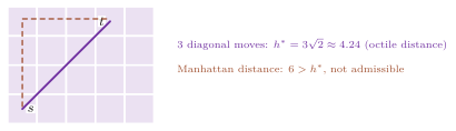
On a grid with 8 moves the Manhattan distance is not admissible,
whatever the cost of a diagonal move between 1 and \(\sqrt{2}\). For
instance, three diagonal moves of unit cells cost \(3\sqrt{2} \approx
4.24\), while the Manhattan distance of their ends is 6 (Figure
5.1); the Euclidean distance is admissible
there, and consistent, but it is weaker than the octile distance, which
is the distance of the relaxation without walls. Finally, the sequence
score of Nilsson (SequenceScore.h) adds to the Manhattan
distance a term that counts the tiles out of sequence; it is not admissible,
and A\(^*\) then usually expands fewer nodes, but it may return a path that is
not optimal (§2.4).
5.3 The abstraction of a pattern¶
In a sliding-tile puzzle, the board has \(n = W H\) cells, and a state
\(s\) places the tiles \(1, \ldots, n - 1\) and the blank on distinct
cells; a move exchanges the blank with a tile in an adjacent cell, at
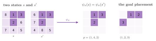
cost 1. A pattern is a set \(\pi = \{t_1, \ldots, t_k\}\) of tiles,
and the placement of \(\pi\) in \(s\) is the vector
\(p = \psi_\pi(s) = (q_{t_1}, \ldots, q_{t_k})\) of the cells of its
tiles, the other tiles being "don't care"
(Figure 5.2).
Thus, the placements are the \(k\)-permutations of the \(n\) cells, i.e.,
\(N = n! / (n - k)!\) of them, and the goal placement is the placement
of the goal. In this chapter \(\pi\) denotes a pattern, as in the
literature of the pattern databases and in the comments of
PatternDatabase.h, and not a path as in Table 1.2 of
§1.4. In the library, TilePattern
(PatternDatabase.h:243) takes a pattern as the list
of its tiles, in a chosen order, and the board of the goal. Its constructor
refuses a goal that is not a permutation of the cells
(PatternDatabase.h:289), an empty pattern or one of
more than \(n - 2\) tiles (:292), and a tile outside \(1, \ldots, n - 1\) (the
blank, in particular) or a tile given twice (:300).
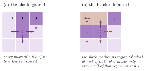
The abstract space of \(\pi\) is a graph on the placements whose edges
move one tile of \(\pi\) to an adjacent cell, at cost 1. As Figure
5.3 shows, the library builds it under two
rules of the blank (BlankRule,
PatternDatabase.h:204).
- With the blank ignored, an abstract state is a placement, and each move of a tile of \(\pi\) to an adjacent cell free of the other tiles of \(\pi\) is allowed, as if the blank were wherever needed. The table holds the distance \(d_\pi(p)\) from \(p\) to the goal placement in this graph, which is undirected and has unit costs.
- With the blank minimized, an abstract state is a placement together with the cell \(b\) of the blank, a move of the blank into a cell that no tile of \(\pi\) holds costs 0 (it moves a tile out of the pattern), and a move of a tile of \(\pi\) into the cell of the blank costs 1. The blank thus reaches at no cost each cell of its region, i.e., of its connected component among the cells free of \(\pi\), and the table holds the least distance over the cells of the blank, \(d_\pi(p) = \min_b d_\pi(p, b)\); this is the rule of the disjoint databases of [22].
In both cases a move of the puzzle that moves a tile of \(\pi\) is an edge of cost 1 of the abstract space. A move of any other tile changes no placement (with the blank ignored) or is an edge of cost 0 (with the blank minimized); hence \(\psi_\pi\), with the cell of the blank added in the second case, is an abstraction in the sense of Definition 5.1. We now compare the two rules.
Lemma 5.3 (The minimized blank dominates). For each placement \(p\), \(d_\pi(p)\) with the blank minimized is at least \(d_\pi(p)\) with the blank ignored.
Proof. A path of the minimized space from \((p, b)\) to the goal, deprived of its moves of the blank, is a sequence of moves of the tiles of \(\pi\), each into a cell free of the other tiles of \(\pi\), i.e., a path of the space with the blank ignored, of the same cost. Hence the distance with the blank ignored is at most \(d_\pi(p, b)\) for each \(b\), and at most their minimum. \(\square\)
Note that the test pdb checks the values of the tables, under both
rules, against a breadth-first search of the abstraction written apart
from the library, on each placement of patterns of 1 to 7 tiles of the
8-puzzle and with two goals; it does not compare the two rules with each
other, and Lemma 5.3 rests on its proof.
5.4 Ranking the placements¶
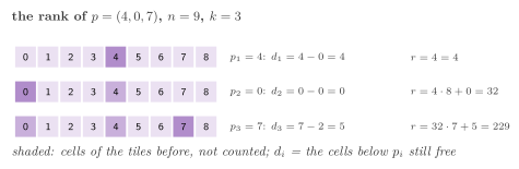
A table is an array indexed by the placements, which need a perfect ranking, i.e., a bijection \(\mathrm{rank}\) from the placements onto \([0, N)\), computed at each lookup. We rank a placement as a \(k\)-permutation in lexicographic order: the digit of the \(i\)-th tile is the number \(d_i\) of the cells below \(p_i\) that the tiles before it do not hold, and
which is the number \(d_1 d_2 \cdots d_k\) written in the mixed radix \((n, n - 1, \ldots, n - k + 1)\), the \(i\)-th digit \(d_i\) being in \([0, n - i + 1)\) since \(p_i\) has at most \(n - i + 1\) free cells below it, itself excluded (Figure 5.4).
TilePattern::rank and TilePattern::unrank compute the map and its
inverse by Algorithm 5.1, in which the set \(U\) of the cells already
used, and the set \(F\) of the free ones, are words of \(n \le 32\) bits.
Hence the count of line 4 is one population count of \(U\) restricted to
the cells below \(p_i\), and the selection of line 13 clears the \(d_i\)
lowest bits of \(F\), one at a time, and takes the lowest one left.
Algorithm 5.1 (RANK and UNRANK, the lexicographic rank of a placement of \(k\) tiles on \(n\) cells).
 1  function RANK(p)              ▷ p = (p_1, …, p_k), distinct cells
 2     r ← 0;  U ← ∅              ▷ U: the cells of the tiles before
 3     for i ← 1 to k do
 4        d_i ← p_i − |{c ∈ U : c < p_i}|
 5        r ← r · (n − i + 1) + d_i
 6        U ← U ∪ {p_i}
 7     return r
 8  function UNRANK(r)            ▷ 0 ≤ r < N
 9     for i ← k down to 1 do
10        d_i ← r mod (n − i + 1);  r ← r div (n − i + 1)
11     F ← {0, 1, …, n − 1}       ▷ the free cells
12     for i ← 1 to k do
13        p_i ← the (d_i + 1)-th least cell of F;  F ← F ∖ {p_i}
14     return p
Lemma 5.4 (The rank is a bijection). (i) The map \(\mathrm{rank}\) is a bijection from the \(k\)-permutations of \(n\) cells onto \([0, n! / (n - k)!)\), RANK computes it in \(O(k)\) operations on words of \(n\) bits, and UNRANK computes its inverse in \(O(k + \sum_i d_i) = O(k\,n)\) of them. (ii) Two ranks \(r\) and \(r'\) with \(\lfloor r / (n - k + 1) \rfloor = \lfloor r' / (n - k + 1) \rfloor\), i.e., in the same block of \(n - k + 1\) consecutive ranks, are the ranks of placements that differ only in the cell of the last tile.
Proof. (i) The cells below \(p_i\) are \(p_i\), of which \(|\{c \in U : c < p_i\}|\) are used, and hence line 4 computes the digit \(d_i\); lines 3 to 6 evaluate the mixed radix sum by the rule of Horner. The mixed radix representation is a bijection from the vectors of digits with \(d_i \in [0, n - i + 1)\) onto \([0, \prod_i (n - i + 1)) = [0, n! / (n - k)!)\), and lines 9 and 10 compute its inverse. The map from a placement to its digits is a bijection too: given the cells \(p_1, \ldots, p_{i-1}\), the cell \(p_i\) is the \((d_i + 1)\)-th of the \(n - i + 1\) cells that they leave free, in increasing order, which is line 13, so that \(p\) is rebuilt from its digits one cell after the other. Each iteration of lines 3 to 6 takes \(O(1)\) operations, and that of lines 12 and 13 takes \(O(1 + d_i)\), one per bit cleared. (ii) The digit of the last tile is \(d_k = r \bmod (n - k + 1)\), and the other digits are those of \(\lfloor r / (n - k + 1) \rfloor\); two ranks of the same block thus have the same digits \(d_1, \ldots, d_{k-1}\), hence by (i) the same cells of the first \(k - 1\) tiles. \(\square\)
Thus, the entries of one block are the placements that differ in the cell of the last tile, which the max-compression of §5.9 exploits. The linear-time ranking of Myrvold and Ruskey [34] would do as well, and it does without the population counts (it serves the permutation puzzles, §5.14). The lexicographic one keeps close placements in close entries, as (ii) shows, and its cost of \(k\) population counts is small against the cache miss that the lookup of a large table pays anyway (a judgement on the hardware, not a theorem).
5.5 Building a table¶
Each table is filled by a breadth-first search of the
abstract space, backward from the goal placement and by layers: at the
layer \(d\) each entry of value \(d\) is expanded, and its neighbours not
seen yet get the value \(d + 1\); the search ends when a layer adds no
entry. Since the abstract space with the blank ignored is undirected,
the backward distances are the forward ones. We give the pseudocode of
the Doxygen comment of PatternDatabase.h.
Algorithm 5.2 (BUILD-IGNORED, the table of a pattern with the blank ignored).
 1  procedure BUILD-IGNORED(π)               ▷ the blank ignored
 2     for each r ∈ [0, N) do h[r] ← ∞          ▷ N = n! / (n − k)!
 3     h[rank(goal(π))] ← 0;  d ← 0
 4     loop
 5        new ← 0
 6        for each r with h[r] = d do        ▷ by blocks, in parallel
 7           p ← unrank(r)
 8           for each tile i of π, each cell c next to p_i, c ∉ p do
 9              r' ← rank(p with p_i ← c)
10              if h[r'] = ∞ then          ▷ by compare-and-swap
11                 h[r'] ← d + 1;  new ← new + 1
12        if new = 0 then return h
13        d ← d + 1
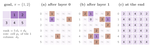
Figure 5.5 follows Algorithm 5.2 on the board of \(3 \times 2\) cells with the pattern \(\{1, 2\}\), whose 30 placements are laid out by rank as a \(6 \times 5\) matrix: the layer 0 is the goal placement, the layer 1 its three neighbours, and the table is complete after the layer 5.
Each layer is scanned in blocks of \(2^{14}\) consecutive ranks, which the
workers of a runtime take from a shared counter, each block at a time.
The entries take one byte each during the construction, with the value
255 standing for \(\infty\), and an entry is claimed by an atomic
compare-and-swap from 255 to \(d + 1\) (line 10): of the workers that try
to claim the same entry in a layer, exactly one succeeds and counts it
in new, and the others fail and count nothing. A layer \(d\) with \(d + 1
\ge 255\) throws std::logic_error
(PatternDatabase.h:1507), and a placement still at
255 at the end makes PatternTable::distances throw too
(PatternDatabase.h:1137). A pattern of \(k = n - 1\)
tiles, for which the abstraction would be the puzzle itself and only half of
the placements would be reachable (Exercise 5.3), is refused by the constructor
of TilePattern; for \(k \le n - 2\) we do not prove that each placement is
reachable, and the throw is the check of it. Also, the test that throws is made
at the start of each layer \(d\) with \(d + 1 \ge 255\), before the entries of that
layer are scanned; hence a table whose largest distance is exactly 254 is
refused too (no table of the library comes near that value).
With the blank minimized the states are the pairs \((p, b)\), with \(b\) coded by its index among the \(n - k\) cells free of the pattern. Each state takes 2 bits (unseen, current, next, old), as in the two-bit breadth-first search of Korf [26]. A state is expanded once per region, from the least cell of the region, and its successors are marked together with all the cells of the region of the blank after the move, which realizes the moves of cost 0 without a second queue.
Algorithm 5.3 (BUILD-MINIMIZED, the table of a pattern with the blank minimized).
 1  procedure BUILD-MINIMIZED(π)             ▷ the blank minimized
 2     S[r, b] ← unseen for each r and each cell b ∉ unrank(r)
 3     S[rank(goal(π)), b] ← current for each b ∉ goal(π)
 4     h[r] ← ∞ for each r;  h[rank(goal(π))] ← 0;  d ← 0
 5     loop
 6        for each (r, b) with S[r, b] = current do    ▷ in parallel
 7           p ← unrank(r);  R ← region(p, b)  ▷ the cells b reaches
 8           if b ≠ min R then continue      ▷ one cell per region
 9           for each c ∈ R, each tile i of π with p_i next to c do
10              p' ← p with p_i ← c;  r' ← rank(p')
11              for each b' ∈ region(p', old p_i) do
12                 if S[r', b'] = unseen then S[r', b'] ← next
13              if h[r'] = ∞ then h[r'] ← d + 1
14        if no state is next then return h
15        S ← S with current → old and next → current;  d ← d + 1
Line 3 starts from the goal placement with the blank anywhere, since the
backward search looks for the states from which the goal placement is
reached, with the blank wherever it ends. Line 11 marks the whole region
of the blank after the move, which contains the cell left by the tile,
since the states of a region are at the same distance (the blank moves
within it at no cost), and line 13 writes the table of the placements.
Both marks are made by a compare-and-swap, as in Algorithm 5.2. The
patterns of a partition are built one after the other, each with all
the workers (PDBOptions::threads, all the cores if 0). We now prove
that the two procedures compute the tables, whatever the interleaving
of the workers, and give their cost.
Theorem 5.5 (The construction of the tables). Let \(D\) be the largest distance in the table. (i) Algorithm 5.2, with the layers scanned by any number of workers in any interleaving, gives each entry the distance \(d_\pi\) of its placement from the goal placement in the space with the blank ignored. (ii) Algorithm 5.3, in the same conditions, gives each entry \(\min_b d_\pi(p, b)\), the least distance in the space with the blank minimized over the cells \(b\) of the blank. (iii) Algorithm 5.2 takes \(O(N (D + k\,n))\) operations and \(N\) bytes; Algorithm 5.3 takes \(O(N (n - k)(D + k\,n))\) operations, \(N\) bytes for the table and \(N (n - k) / 4\) bytes for the states.
Proof. (i) We show by induction on \(d\) that at the start of the layer \(d\) the entries of value at most \(d\) are the placements at distance at most \(d\), with their distances, and the others are \(\infty\); it holds for \(d = 0\) by line 3. During the layer \(d\), the workers read the entries equal to \(d\) and write only the value \(d + 1\) into entries equal to \(\infty\). Hence the set of the entries equal to \(d\) does not change during the layer, whatever the interleaving; each neighbour of such an entry that was \(\infty\) at the start of the layer is set to \(d + 1\) by exactly one compare-and-swap; and no other entry changes. The placements so set are those at distance \(d + 1\): a placement at distance \(d + 1\) has a neighbour at distance \(d\) (the space being undirected, the next placement of a shortest path to the goal), and a neighbour of a placement at distance \(d\) is at distance at most \(d + 1\), hence exactly \(d + 1\) if it was \(\infty\). The search ends at the first layer that sets no entry, when every placement reachable from the goal has its distance. (ii) The moves of the space with the blank minimized are reversible at the same cost: a tile of \(\pi\) moved from \(a\) into the blank \(b\) moves back from \(b\) into the blank, now in \(a\), and a move of the blank inside a region is undone by the opposite move. The space is thus undirected, the distance \(d_\pi(p, b)\) is constant over the cells \(b\) of a region, and the states at distance \(d + 1\) are those that are not at distance at most \(d\) and are reached from a state at distance \(d\) by one move of cost 1 followed by moves of cost 0 (a shortest path from such a state to the goal begins with moves of cost 0 inside its region and then makes a move of cost 1, read backward). Lines 7 to 12 enumerate, from the least cell of each region of the layer \(d\), every cell \(c\) of the region and every tile of \(\pi\) next to it, which are all the moves of cost 1 out of the states of the region, and line 11 marks the whole region of the new blank. By the induction of (i), with the 2 bits in place of the entries, the states marked current at the start of the layer \(d\) are those at distance \(d\), the old ones those at a smaller distance, and the marks of the layer are those at distance \(d + 1\). Line 13 writes \(d + 1\) into \(h[r']\) only if no state of the placement \(r'\) has been reached before, i.e., at the least \(d\) at which some state \((r', b')\) is at distance \(d\), which is \(\min_b d_\pi(p, b)\). (iii) Each layer scans the \(N\) entries, or the \(N (n - k) / 32\) words of the states, and there are \(D + 2\) layers. With the blank ignored, each placement is expanded once, at the layer of its distance, by one unrank of \(O(k\,n)\) operations and at most \(4 k\) moves with as many ranks of \(O(k)\) operations, i.e., \(O(k\,n + k^2) = O(k\,n)\) operations by Lemma 5.4. With the blank minimized, each state is current in one layer only and costs an unrank, of \(O(k\,n)\) operations, and the computation of its region, of \(O(n)\) operations, since the region grows by one step of adjacency per operation on its word; the least state of a region also makes, for each of its cells, the at most 4 tests of a neighbour, and for each of the at most \(4 k\) pairs of a cell of the region and a tile next to it a rank, a region and the marks of that region, i.e., \(O(k + n)\) operations each. The memory is that of the arrays. \(\square\)
The test pdb checks (i) and (ii) against a breadth-first search of
the abstraction written apart from the library, on 1 and on 3 workers.
The bounds of (iii) are linear in \(N\) for a fixed size of the pattern
and a fixed largest distance \(D\).
5.6 Additive pattern databases¶
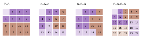
Clearly, the table of one pattern is a rather weak heuristic, since it ignores the other tiles. Taking the maximum of the tables of several patterns is admissible (Lemma 2.5), but it is not much stronger than the best of them; the sum is much stronger, and it is admissible when the patterns are disjoint and each table counts only the moves of its own tiles. Let \(\pi_1, \ldots, \pi_m\) be disjoint patterns (a partition of the tiles, or of a subset of them; Figure 5.6), and let
Theorem 5.6 (Admissibility of the additive heuristic). If the patterns are disjoint and none holds the blank, \(h\) is admissible, with either rule of the blank, and \(h = 0\) at the goal.
Proof. Consider a path \(P\) from \(s\) to the goal, and let \(c_j(P)\) be the number of its moves that move a tile of \(\pi_j\). The projection of \(P\) on \(\pi_j\) (with the cell of the blank, under the minimized rule) is a path of the abstract space from \(\psi_{\pi_j}(s)\) to the goal placement whose cost is \(c_j(P)\), since the moves of the other tiles cost nothing there. Hence \(d_{\pi_j}(\psi_{\pi_j}(s)) \le c_j(P)\) (with the minimized rule, \(d_{\pi_j}\) is the minimum over the cells of the blank, and the projection starts from one of them). Each move of the puzzle moves one tile, which belongs to at most one pattern; thus \(\sum_j c_j(P) \le c(P)\), and summing over \(j\) gives \(h(s) \le c(P)\) for each path, i.e., \(h(s) \le h^*(s)\). At the goal each placement is the goal placement, of distance 0. \(\square\)
This is the argument of Korf and Felner
[22], which Yang et al.
[28] cast for any family of abstractions
whose costs split the cost of each edge. This argument needs the
patterns to be disjoint and the abstract spaces to charge only the moves
of their tiles. For this reason the blank belongs to no pattern: a table
that charged the moves of the blank would count each move twice, once
for the blank and once for the tile. AdditivePDB
(PatternDatabase.h:1733) refuses a tile in two
patterns, and TilePattern refuses the blank. In fact, the Manhattan distance
is the additive database of the \(n - 1\) patterns of one tile each, and a
partition into larger patterns dominates it (Proposition
5.14). The partitions of Figure
5.6 are given by the functions
partition_15_7_8(), partition_15_5_5_5(), partition_15_6_6_3() and
partition_24_6_6_6_6() of PatternDatabase.h.
The heuristic of a state \(s\) is computed from the array \(q\) of the
cells of all the tiles, \(q[t]\) being the cell of the tile \(t\) and
\(q[0]\) that of the blank. Algorithm 5.4 gives the lookup H of
AdditivePDB::heuristic (the maximum with the reflection of
§5.8, when it is used), the value VALUE of
an entry for each encoding of §5.9, in
which \(m_j(p)\) is the Manhattan distance of the tiles of \(\pi_j\) read
from a table of \(k_j n\) bytes and \(e_j\) the stored excess, and the
heuristic CHILD-H of a successor, which SlidingTilePDB computes for
each successor that it generates; DELTA and the residues \(\mathrm{res}_j\)
belong to the relative encodings of §5.9.
Algorithm 5.4 (The lookups of an additive pattern database).
 1  function H(q)
 2     a ← SUM(q)
 3     if not reflected then return a
 4     for each tile t, the blank included, do q'[σ(t)] ← T(q[t])
 5     return max(a, SUM(q'))              ▷ q': the reflection of s
 6  function SUM(q)
 7     v ← 0
 8     for each pattern π_j do
 9        p ← (q[t] for the tiles t of π_j, in their order)
10        v ← v + VALUE_j(RANK_j(p), m_j(p))
11     return v
12  function VALUE_j(r, m)                 ▷ by the encoding of the table
13     byte: d_j[r];  nibble: m + 2 e_j[r];  min: m + 2 e_j[r div c]
14     sparse: m if B_j[r] = 0, else m + 2 x_j[rank₁(B_j, r)]
15  function CHILD-H(q, h, x, b)   ▷ the tile x moves into the blank cell b
16     if the encoding is relative then return h + DELTA(q, x, b)
17     a ← q[x];  q[x] ← b;  q[0] ← a
18     v ← H(q);  q[x] ← a;  q[0] ← b
19     return v
20  function DELTA(q, x, b)
21     if x belongs to no pattern then return 0
22     j ← the pattern of x
23     y ← res_j(q);  y' ← res_j(q with q[x] ← b)
24     return ((y' − y + 1) mod M) − 1
The symbols of Algorithm 5.4 that the later sections define are the
following: \(T\) and \(\sigma\) of line 4 are the transposition of the cells
and the renaming of the tiles of the reflection
(§5.8); in line 13, \(d_j\) is a table of
bytes, \(e_j\) a table of stored excesses and \(c\) the group of
MinNibbleEntries; in line 14, \(B_j\) is the bit vector of
SparseEntries, \(\mathrm{rank}_1(B_j, r)\) the number of its ones before
the position \(r\) and \(x_j\) the array of its nonzero excesses
(§5.9); and \(M\) in line 24 is 3 or 4
(Lemma 5.10). Line 17 makes \(q\) the array
of the successor (the tile \(x\) in the cell
\(b\), the blank in the cell that \(x\) leaves), and line 18 restores it, so
that the same array serves all the successors of \(s\). Thus,
SlidingTilePDB (PatternDatabase.h:1935) is the
domain SlidingTile whose heuristic is that of an AdditivePDB, and each
search of the library runs on it unchanged; it calls H, or EXACT of
§5.9 with a relative encoding, only for the
initial state, and CHILD-H for each successor. Proposition
5.13 gives the cost of these functions.
The options of the construction, and the classes that a user declares, are the following; the first excerpt is from the header, the constructors are quoted by hand, since in the header they come with their bodies.
enum class BlankRule : std::uint8_t {
 ignored ,   ///< the blank is not in the abstract state: consistent tables
 minimized   ///< the blank is, and the table keeps the least distance
 };

/*- - - - - - - - - - - - - - - - - - - - - - - - - - - - - - - - - - - - -*/
/// a partition of the tiles into disjoint patterns

using Partition = std::vector< std::vector< int > >;

/*- - - - - - - - - - - - - - - - - - - - - - - - - - - - - - - - - - - - -*/
/// the options of the construction of an AdditivePDB

struct PDBOptions {
 BlankRule blank = BlankRule::ignored;     ///< the rule of the blank
 bool reflect = true;          ///< also the reflection, where it is valid
 unsigned compress = 1;        ///< ranks per entry of MinNibbleEntries
 unsigned threads = 0;         ///< workers of the construction (0: all)
 std::string cache;            ///< directory of the tables ("": none)
 };
template< int W , int H , class Enc = NibbleEntries >
class AdditivePDB {
 public:
 AdditivePDB( const Partition & partition ,
              const board_type & goal = Pattern::korf_goal() ,
              const PDBOptions & o = {} );
 [[nodiscard]] int heuristic( const std::uint8_t * q ) const;
 [[nodiscard]] bool reflected( void ) const;
 };

template< int W , int H , class Enc = NibbleEntries >
class SlidingTilePDB : public SlidingTile< W , H > {
 public:
 SlidingTilePDB( const board_type & start ,
                 const AdditivePDB< W , H , Enc > & pdb );
 };
The constructor of AdditivePDB builds the table of each pattern, or
takes it from the directory cache (§5.10),
with threads workers, and reflect asks for the reflection where it
is valid; compress is the group \(c\) of MinNibbleEntries. A second
constructor takes the tables already built, and make() builds them on
another runtime of the workers (§1.6).
heuristic requires an absolute encoding, exact (H with EXACT in
place of VALUE) and delta (DELTA) a relative one. The SlidingTilePDB
keeps a reference to the AdditivePDB, which must outlive it, and it
refuses a relative encoding with the reflection
(§5.9). The following test case builds the
partition 4-4 of the 8-puzzle with two encodings and searches with
both.
PDBOptions o;
o.blank = BlankRule::ignored;   // consistent tables (the default)
o.reflect = true;               // also the reflection about the diagonal
o.threads = 2;                  // workers of the construction
// a directory in o.cache: the tables built once, then read from there
const Partition part{ { 1 , 2 , 3 , 4 } , { 5 , 6 , 7 , 8 } };
const AdditivePDB< 3 , 3 > pdb( part , EightPuzzle::korf_goal() , o );
const auto board = EightPuzzle::parse( "7 2 4 5 0 6 8 3 1" );
const SlidingTilePDB< 3 , 3 > d( board , pdb );
const auto s = astar( d );      // s.cost and s.stats.expanded
// the residues modulo 3 need the tables without the reflection
o.reflect = false;
const AdditivePDB< 3 , 3 , Mod3Entries > pdb3( part ,
                                               EightPuzzle::korf_goal() ,
                                               o );
const SlidingTilePDB< 3 , 3 , Mod3Entries > d3( board , pdb3 );
const auto s3 = astar( d3 );
5.7 Consistency¶
With the blank ignored the additive heuristic is consistent, and the proof gives a finer property of the tables, on which the encodings of §5.9 rest. Let \(m_\pi(p)\) be the Manhattan distance of the tiles of \(\pi\) in the placement \(p\).
Lemma 5.7 (Parity and excess). With either rule of the blank, \(d_\pi(p) \ge m_\pi(p)\) and \(d_\pi(p) \equiv m_\pi(p) \pmod 2\) for each placement \(p\). With the blank ignored, two adjacent placements \(p\) and \(p'\) have \(|d_\pi(p) - d_\pi(p')| = 1\).
Proof. A move of cost 1 moves one tile of \(\pi\) by one cell, and hence changes \(m_\pi\) by exactly one unit, while a move of cost 0 (of the blank, with the minimized rule) does not change it. Along a path of least cost from \(p\) to the goal placement, where \(m_\pi = 0\), the value of \(m_\pi\) thus goes to 0 by \(d_\pi(p)\) steps of \(\pm 1\), which gives both claims of the first sentence. With the blank ignored, the abstract space is undirected with unit costs, so that \(|d_\pi(p) - d_\pi(p')| \le 1\) for adjacent placements, and the parity of \(d_\pi\), which is that of \(m_\pi\), differs between them, since \(m_\pi(p)\) and \(m_\pi(p')\) differ by one; hence the difference is not zero. \(\square\)
Theorem 5.8 (Consistency with the blank ignored). With the blank ignored, the additive heuristic of disjoint patterns is consistent.
Proof. A move of the puzzle moves one tile; if it belongs to no pattern, no placement changes and \(h\) does not change; otherwise only the placement of its pattern changes, to an adjacent one, and by Lemma 5.7 \(h\) changes by one. In either case \(h(s) \le 1 + h(s')\) for each move \((s, s')\), and \(h = 0\) at the goal by Theorem 5.6. \(\square\)
With the blank minimized, the same move may change the value of a table
by more than one. In fact, the minimum over the cells of the blank
forgets in which region the blank actually is, and the region that the
true blank occupies after the move may be far from the one that realized
the minimum before it. Hence, the sum is admissible but usually not
consistent. On the 8-puzzle with the goal of Korf and the partition
4-4, the two ends of 18840 of its 241920 moves differ by more than one
without the reflection, and of 16986 with it, as a computation of the
tables written apart from the library gives (the test pdb prints the
same counts as ordered pairs of a state and a successor, i.e., twice
these numbers), and A\(^*\) stays optimal by reopening the closed nodes
(§2.7 and [31]).
In exchange, the heuristic is larger: by Lemma
5.3 each table with the blank minimized is at
least the one with the blank ignored, which in turn is at least the
Manhattan distance of its tiles (Lemma 5.7);
PDBBench --mode table reports the mean of each heuristic on \(10^6\)
random states (column mean_h), against that of the Manhattan distance
(column mean_manhattan). By default, PDBOptions has the blank
ignored, which all the encodings accept and which keeps the heuristic
consistent; the sequential A\(^*\) then never expands a node twice. One
chooses the blank minimized explicitly, as in the example of
§5.6.
5.8 The reflection about the main diagonal¶
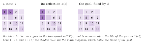
Let the board be square, and let the goal have the blank on the main diagonal, as the goal of Korf (the blank in the first cell) does. The transposition \(T\) of the cells, \(T(\text{row } i, \text{column } j) = (\text{row } j, \text{column } i)\), maps adjacent cells to adjacent cells. Let \(\sigma(t)\) be the tile that the goal holds in the cell \(T(c^*_t)\), with \(c^*_t\) the goal cell of \(t\), and let \(\phi(s)\) be the state that holds the tile \(\sigma(t)\) in the cell \(T(q_t)\), for each tile \(t\) of \(s\) (the blank included, Figure 5.7).
Lemma 5.9 (The reflection is an automorphism). The map \(\phi\) is a bijection of the states, maps the moves of the puzzle to moves, and fixes the goal; hence \(h^*(\phi(s)) = h^*(s)\) for each state \(s\).
Proof. Since \(T\) and \(\sigma\) are bijections, so is \(\phi\). The blank is fixed by \(\sigma\), since \(T(c^*_0) = c^*_0\) when the goal cell of the blank is on the diagonal. A move of \(s\) exchanges the blank, in the cell \(b\), with the tile \(x\) in an adjacent cell \(a\); in \(\phi(s)\) the blank is in \(T(b)\) and \(\sigma(x)\) in \(T(a)\), which is adjacent to \(T(b)\), and exchanging them gives \(\phi\) of the successor. The goal holds \(t\) in \(c^*_t\), and \(\phi\) puts in \(T(c^*_t)\) the tile \(\sigma(t)\), which is by definition the tile of the goal in \(T(c^*_t)\), i.e., it gives the goal back. Hence \(\phi\) maps the paths from \(s\) to the goal onto the paths from \(\phi(s)\) to the goal, of the same costs. \(\square\)
Thus, the sum of the same tables on \(\phi(s)\) is another admissible heuristic of \(s\), since \(h(\phi(s)) \le h^*(\phi(s)) = h^*(s)\), and it is consistent if \(h\) is, since \(\phi\) maps moves to moves; the library takes
which is the reflection of [22], admissible
and, with the blank ignored, consistent by
Lemma 2.5. The reflection costs a second
lookup per table; it is used only when it is valid, i.e., on a square
board whose goal has the blank on the diagonal, and when
PDBOptions::reflect asks for it (AdditivePDB::reflected() tells
whether it is used). The constructor of AdditivePDB computes the
arrays \(T\) and \(\sigma\) once, in \(O(n)\) time, and line 4 of Algorithm
5.4 builds the cells of \(\phi(s)\) from them: the tile \(\sigma(t)\) of
\(\phi(s)\) is in the cell \(T(q_t)\).
The dual lookup of Zahavi et al. [29], which looks up the placement of the inverse permutation of the state, is another admissible lookup of the same tables; it is not consistent, and it pays off with the bidirectional pathmax of IDA\(^*\), which the library does not have.
5.9 The encodings of the entries¶
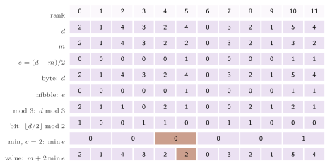
A table of the partition 7-8 of the 15-puzzle has more than half a billion entries (§5.11), and the memory of the entries decides both whether the tables fit and how often a lookup misses the cache. Let \(e_\pi(p) = (d_\pi(p) - m_\pi(p)) / 2\) be the excess of the distance over the Manhattan distance of the tiles of the pattern; by Lemma 5.7 it is a nonnegative integer, typically much smaller than the distance (cf. Figure 5.8). At the lookup, the Manhattan distance of the tiles is computed from a table of \(k n\) bytes, and the entries store the excess, or less. We list the encodings of the library below (Figure 5.8).
ByteEntries(PatternDatabase.h:526) stores \(d_\pi\) in 8 bits per entry.NibbleEntries(PatternDatabase.h:591, the default) stores \(e_\pi\) in 4 bits per entry, saturated at 15; the value is \(m_\pi + 2 e_\pi\). A saturated entry gives a smaller value, which is still admissible, andclamped()counts them (the testpdbchecks that the tables of the 8-puzzle have none).Mod3Entries(PatternDatabase.h:679) stores \(d_\pi \bmod 3\), five residues in a byte as the digits of a number in base 3 (\(3^5 = 243 \le 256\)), i.e., \(8 / 5 = 1.6\) bits per entry, after Breyer and Korf [25].ParityBitEntries(PatternDatabase.h:758) stores \(\lfloor d_\pi / 2 \rfloor \bmod 2\), one bit per entry: with the parity of \(d_\pi\), which is that of \(m_\pi\), it gives \(d_\pi \bmod 4\), as in the 1-bit encoding of Clausecker and Reinefeld [27].MinNibbleEntries(PatternDatabase.h:838) stores, for each group of \(c\) consecutive ranks (\(c\) a power of 2,PDBOptions::compress), the least excess of the group in 4 bits, i.e., \(4 / c\) bits per entry: the lossy max-compression of Felner et al. [24], which here keeps the Manhattan distance of each placement exact.SparseEntries(PatternDatabase.h:940) stores a bit per entry that records whether its excess is nonzero, with a directory of rank and select of about \(0.4\) bits per entry, and the nonzero excesses in 4 bits each, in the order of their ranks; it is smaller thanNibbleEntrieswhen fewer than about 65% of the excesses are nonzero, at the price of a rank per lookup.
The values of ByteEntries, of NibbleEntries when no entry saturates,
and of SparseEntries (which saturates in the same way) when no entry
saturates, are the distances themselves, so that they are admissible and
consistent as in §5.6 and
§5.7. Each of the other three needs an
argument.
The relative encodings¶
In Mod3Entries and ParityBitEntries, the residues do not give the
value of a placement, but they give the change of the value along a
move.
Lemma 5.10 (The change from the residues). With the blank ignored, let \(p\) and \(p'\) be adjacent placements and \(r\), \(r'\) the residues of their distances modulo \(M \in \{3, 4\}\). Then
Proof. By Lemma 5.7 the difference \(\delta\) is \(+1\) or \(-1\). If \(\delta = 1\), then \(r' - r \equiv 1\) and the right-hand side is \(2 - 1 = 1\); if \(\delta = -1\), then \(r' - r \equiv -1\), \((r' - r + 1) \bmod M = 0\), and the right-hand side is \(-1\). Both cases are told apart since \(1 \not\equiv -1 \pmod M\) for \(M \ge 3\). \(\square\)
A move of the puzzle moves the tile of one pattern only, so that the
heuristic of a successor is that of its parent plus the change of one
table. This is DELTA in Algorithm 5.4 (AdditivePDB::delta()), whose
line 24 is the formula of Lemma 5.10, and CHILD-H calls it for each
successor; A\(^*\) thus never needs the absolute value but for the initial state.
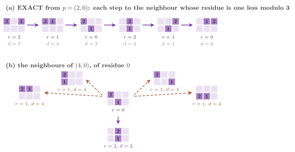
That one is found from the residues only, by a descent to the goal
(Figure 5.9).
Theorem 5.11 (The value from the residues). With the blank ignored, starting from a placement \(p\) and moving each time to a neighbour whose residue is that of the current placement minus one modulo \(M\), one reaches the goal placement in exactly \(d_\pi(p)\) steps; such a neighbour exists at each step before the goal.
Proof. Let \(q\) be the current placement, not the goal. The abstract space is undirected with unit costs, and the next placement on a path of least cost from \(q\) to the goal is a neighbour of distance \(d_\pi(q) - 1\), whose residue is \(r - 1 \bmod M\). Each neighbour has distance \(d_\pi(q) \pm 1\) (Lemma 5.7), and those of distance \(d_\pi(q) + 1\) have residue \(r + 1 \bmod M \ne r - 1 \bmod M\); hence each neighbour with the residue sought is one step closer, and the descent reaches the goal placement, the only one of distance 0, after exactly \(d_\pi(p)\) steps. \(\square\)
The descent is Algorithm 5.5 (PatternTable::exact()), which throws
std::logic_error if it finds no neighbour with the residue sought, a
case that Theorem 5.11 excludes for the tables that the library builds.
Algorithm 5.5 (EXACT, the value of a placement from the residues
alone; \(M = 3\) for Mod3Entries, 4 for ParityBitEntries).
1  function EXACT_j(p)
2     v ← 0
3     while p ≠ goal(π_j) do
4        y ← (res_j(p) − 1) mod M
5        p ← a neighbour p' of p, i.e., p with one tile moved to an
6            adjacent cell free of the others, with res_j(p') = y
7        v ← v + 1
8     return v
Each step tries at most \(4 k\) neighbours, i.e., \(4 k\) ranks and lookups; the value of the initial state thus costs \(O(k\, d_\pi(p))\) lookups per table (Proposition 5.13).
We remark that the argument needs adjacent placements to differ by
exactly one, i.e., the blank ignored (the constructor of PatternTable
refuses a relative encoding with the blank minimized,
PatternDatabase.h:1110), and the heuristic to be
the sum of the tables, since from the maximum of two sums the change of one
table cannot be told: this is why SlidingTilePDB refuses a relative encoding
with the reflection (PatternDatabase.h:1958).
The max-compression¶
In MinNibbleEntries, the ranks are grouped by \(c\) consecutive ones,
\(G(p)\) being the group of the rank of \(p\), and the value of \(p\) is
\(m_\pi(p) + 2 \min_{p' \in G(p)} e_\pi(p')\), the least excess being
saturated at 15.
Proposition 5.12 (The max-compression). For each placement \(p\), \(m_\pi(p) \le m_\pi(p) + 2 \min_{p' \in G(p)} e_\pi(p') \le d_\pi(p)\); hence the sum of the max-compressed tables of disjoint patterns is admissible and at least the Manhattan distance of the tiles of the patterns. It is not consistent in general.
Proof. The excesses are nonnegative (Lemma 5.7), which gives the first inequality, and the least excess of the group is at most \(e_\pi(p)\), while the saturation can only lower it, which gives the second, since \(m_\pi(p) + 2 e_\pi(p) = d_\pi(p)\). The sum is then at most the sum of the distances, which is admissible by Theorem 5.6. For the last claim, on the table of Figure 5.5 with \(c = 2\) the adjacent placements \((1, 0)\) and \((2, 0)\), of ranks 5 and 10, have the values 2 and 5 (Exercise 5.10), and a heuristic consistent along a move of cost 1 changes by at most 1. \(\square\)
A\(^*\) may thus reopen nodes on these tables. Felner et al. [24] store the least distance of the group instead of the least excess. Neither value dominates the other in general (the placement of least excess may have a larger Manhattan distance than \(p\), or a smaller one), but only the second is always at least the Manhattan distance of the pattern, by Proposition 5.12; that it loses less on the tables of the sliding-tile puzzles is a motivation, not a theorem. The groups are aligned to \(c\) and the blocks of Lemma 5.4 (ii) to \(n - k + 1\), so that a group with \(c \le n - k + 1\) meets at most two blocks and holds placements that differ mostly in the cell of the last tile.
The cost of the lookups and the size of the patterns¶
Proposition 5.13 (The cost of a lookup). Let
the partition have \(m\) patterns of \(k_1, \ldots, k_m\) tiles, \(\sum_j k_j
\le n - 1\). With an absolute encoding, H of Algorithm 5.4 takes \(O(n)\)
operations and \(m\) accesses to the tables, twice as many with the
reflection, plus one rank of the directory per table with
SparseEntries; CHILD-H takes the same. With a relative encoding,
CHILD-H takes \(O(k_j)\) operations and 2 accesses to the table of the
tile moved, and EXACT of a placement \(p\) of \(\pi_j\) takes \(O(k_j^2\,
d_{\pi_j}(p))\) operations and at most \(4 k_j\, d_{\pi_j}(p) + 1\)
accesses.
Proof. SUM gathers \(k_j\) cells and computes a rank and a Manhattan
distance in \(O(k_j)\) operations per pattern (Lemma
5.4), with one access to the entries, and
line 4 of Algorithm 5.4 takes \(O(n)\); VALUE takes \(O(1)\) operations but
for the rank of SparseEntries. CHILD-H changes two cells of \(q\) and
calls H, or DELTA, which computes two residues of one table. By
Theorem 5.11, EXACT makes \(d_{\pi_j}(p)\)
steps, each of which tries at most \(4 k_j\) moves, each with a rank of
\(O(k_j)\) operations and one access. \(\square\)
Proposition 5.14 (Larger patterns). (i) The additive heuristic of the \(n - 1\) patterns of one tile, with either rule of the blank, is the Manhattan distance. (ii) If \(\pi\) and \(\pi'\) are disjoint, then \(d_{\pi \cup \pi'}(p, p') \ge d_\pi(p) + d_{\pi'}(p')\) for each placement \((p, p')\) of \(\pi \cup \pi'\), with either rule; hence merging two patterns of a partition never decreases the additive heuristic.
Proof. (i) With the blank ignored the abstract space of one tile is the board, in which the distance between two cells is their Manhattan distance. With the blank minimized, the blank reaches every cell but that of the tile at no cost, since the board less one cell is connected on the boards of at least \(2 \times 2\) cells; the tile thus moves to any adjacent cell at cost 1, and the distance is again the Manhattan distance. (ii) A path of the space of \(\pi \cup \pi'\) moves one tile per move of cost 1, each time into a cell free of the tiles of \(\pi \cup \pi'\) (and with the blank minimized, into the region of the blank); its moves of the tiles of \(\pi\) are then moves of the space of \(\pi\), into a cell free of the tiles of \(\pi\) (and of the region of the blank of that space, which contains the region in the larger space), and its other moves change no placement of \(\pi\), or are moves of the blank of cost 0 in the space of \(\pi\). Its cost is thus at least the sum of the costs of its projections on \(\pi\) and on \(\pi'\), which are paths to the goal placements, and at least \(d_\pi(p) + d_{\pi'}(p')\). \(\square\)
By (i), (ii) and Theorem 2.15, a partition into patterns larger than single tiles dominates the Manhattan distance, which is the reason for the patterns; between consistent heuristics, Theorem 2.15 bounds the expansions when the domination is strict on the states that are not goals, and a mere domination bounds them only below the last layer of \(f\).
5.10 Files and the cache of the tables¶
Building the largest tables (the 24-puzzle, the partition 7-8 of the
15-puzzle) is far more expensive than a search on them; hence the tables
are built once and saved. PatternTable::save()
(PatternDatabase.h:1288) writes a table, in
little-endian order, with a header (the magic PBeFSPDB, the version of the
format, the board, the rule of the blank, the code of the encoding and its
parameter, the tiles and the goal), the number of the entries, the length and
the bytes of the payload, and a checksum of everything before it. The file
is written under a temporary name in the same directory and then
renamed; since a rename within a directory replaces the name at once on
the file systems of POSIX, a reader never sees a file half written.
Conversely, load() rejects a file that is truncated, of another
version, whose checksum differs, or that holds another table (another
pattern, goal, rule or encoding), by throwing std::runtime_error. With
a cache directory (PDBOptions::cache), PatternTable::cached()
(PatternDatabase.h:1379) runs Algorithm 5.6, in
which the file of a table is the name that file_name() derives from the
board, the rule, the encoding, its parameter, the tiles and a checksum of the
goal.
Algorithm 5.6 (CACHED, a table from a cache directory).
1  function CACHED(dir, π, rule, Enc, c)
2     if the file of (π, rule, Enc, c) is in dir and loads then
3        return it
4     if the file of (π, rule, byte, 1) is in dir and loads then
5        d ← its distances
6     else d ← BUILD(π, rule);  save d as (π, rule, byte, 1)
7     t ← the encoding Enc of d with the parameter c
8     if (Enc, c) ≠ (byte, 1) then save t as (π, rule, Enc, c)
9     return t
Here BUILD is Algorithm 5.2 or 5.3. A table returned by CACHED is the
encoding of the distances of Theorem 5.5, up to the corruptions of a file
that its checksum does not detect: a checksum of 64 bits detects any
change of a file with a probability close to 1 but not with certainty,
and this is the only claim of this section that we do not prove. The
test pdb checks the round trip, the rejection of a truncated, a
corrupted and a foreign file, and the reuse of the cache.
5.11 Sizes¶
The table of a pattern of \(k\) tiles has \(N = n! / (n - k)!\) entries. The partitions of the library (7-8 and 6-6-6-6 of [22], 6-6-3 and 5-5-5 of [23], on the 15-puzzle or the 24-puzzle as the number in parentheses indicates) give the following sizes, computed from \(N\) and from the bits per entry of each encoding. In the last column we give the max-compression by \(c = 8\) for 7-8 and by \(c = 16\) for 5-5-5, the groups of the benchmark of §5.17. We remark that the entries are summed over the patterns, e.g., \(57657600 + 518918400\) for the patterns of 7 and 8 tiles of the partition 7-8.
| partition | entries | 8 bits | 4 bits | mod 3 | 1 bit | min |
|---|---|---|---|---|---|---|
| 7-8 (15) | 576576000 | 576 MB | 288 MB | 115 MB | 72 MB | 36 MB |
| 6-6-3 (15) | 11534880 | 11.5 MB | 5.8 MB | 2.3 MB | 1.4 MB | |
| 5-5-5 (15) | 1572480 | 1.6 MB | 786 KB | 314 KB | 197 KB | 49 KB |
| 6-6-6-6 (24) | 510048000 | 510 MB | 255 MB | 102 MB | 64 MB |
A table with the blank minimized has the same size (cf. §5.5), but its construction needs \(N (n - k) / 4\) more bytes for the states of Algorithm 5.3, i.e., about 1 GB for the pattern of 8 tiles of the 15-puzzle.
5.12 When the heuristic does not help¶
Recall that the time of a search is the number of its expansions times
the time of an expansion (§2.10). A search
that is too slow is thus too slow for one of these two reasons, and the
counters of the SearchStats usually indicate which one, and what one may try.
- Reexpansions. If
reexpandedis positive, the heuristic is not consistent (Theorem 2.13); a heuristic meant to be consistent then has an error, and an inconsistent one (e.g., the blank minimized) may cost more in reexpansions than it saves in expansions. On a domain whose states can all be enumerated, the tests of the library check the admissibility and the consistency of a heuristic on each state and each move (the 8-puzzle has \(9!/2 = 181440\) states,check_heuristic8intest/test.cpp). The same check on a small instance of a new domain is the quickest diagnosis. - Expansions. The number of expansions is fixed by the heuristic up to
the ties (Theorem 2.14); a stronger
admissible heuristic (larger patterns, the reflection, the blank
minimized) reduces it, and the mean heuristic over a sample of states,
which
PDBBench --mode tablereports, is a first estimate of the gain. If even a heuristic with a large weight does not solve the instance (a weighted A\(^*\), which the library obtains by a wrapper of the domain, §2.2), the instance is probably very hard for any optimal search. If an instance seems never to be solved, one should check that it is solvable at all:SlidingTilerefuses a start whose permutation has the wrong parity (SlidingTile.h:242), while on a grid A\(^*\) proves the absence of a path only after exhausting the component of the start. - Time per expansion. The rate of expansions (
expanded / seconds) falls when the heuristic is costly: a lookup of a table much larger than the cache misses on most expansions, and a smaller encoding (§5.9) may then be faster even with more expansions. The data structures of Chapter 3 are the other cost. - Memory. If the search stops with
Status::node_limit, or the memory runs out,storedmeasures the nodes held. Furthermore, the searches of Chapter 4 trade time for memory, and IDA\(^*\) with a pattern database is the method of [22] for the 24-puzzle (the testtiles24runs it with patterns of 3 tiles).
5.13 The pattern databases of any abstraction¶
The tables of the previous sections rest on the structure of the
sliding-tile puzzles: the rank of a placement, the moves of a tile and
the Manhattan distance of a pattern are those of the board. The header
AbstractionPDB.h gives instead the construction for any
abstraction whose states are ranked, i.e., indexed by the integers of \([0, N)\),
and whose edges have small integer costs; the permutation puzzles of
§5.15 and the Towers of Hanoi of
§5.16 are built on it. Such an abstraction
is described by the concept AbstractSpace, in which size() is \(N\),
for_each_goal( f ) calls f( r ) for each abstract goal \(r\), and
for_each_predecessor( r , f ) calls f( r' , c ) for each edge \((r',
r)\) of cost \(c \in \{1, \ldots, 254\}\); both are const and may be
called by many threads at once.
template< class S >
concept AbstractSpace = requires( const S & s , std::uint64_t r ) {
 { s.size() } -> std::convertible_to< std::uint64_t >;
 s.for_each_goal( detail::rank_sink{} );
 s.for_each_predecessor( r , detail::rank_cost_sink{} );
 };
The edges are meant to be those of an abstraction of the moves of a
domain in the sense of Definition 5.1, so
that the distance of the image of a state is at most the cost of each of
its paths to a goal, and its table is a consistent heuristic by
Proposition 5.2; the concept cannot check
this, which is the responsibility of whoever writes the space. The
table holds, for each abstract state \(r\), the least cost \(\delta(r)\) of
a path from \(r\) to an abstract goal, which abstract_distances( space ,
threads ) computes on threads workers of an executor (all the cores
if 0) by Algorithm 5.7, the pseudocode of the Doxygen comment of the
header. It is the algorithm of Dial [65],
whose buckets are here not lists but the layers of the table itself: the
entries of value \(d\) are final when the layer \(d\) is scanned, since
every edge costs at least 1, and each of them lowers the value of its
predecessors to \(d + c\). The table is cut into blocks of \(2^{14}\)
entries, each with the least value \(\mathrm{lo}[B]\) not yet scanned, so
that a layer skips the blocks that hold none of its entries, which are
most of them in the first and in the last layers.
Algorithm 5.7 (DISTANCES, the table of an abstract space by layers).
 1  procedure DISTANCES(S)
 2     h[r] ← ∞ for each r ∈ [0, N);  h[g] ← 0 for each goal g
 3     lo[B] ← least h of the block B;  next[B] ← ∞
 4     d ← 0
 5     while d < ∞ do
 6        for each block B with lo[B] ≤ d do          ▷ in parallel
 7           m ← ∞
 8           for each r ∈ B do
 9              if h[r] = d then
10                 for each predecessor r' of r, by an edge of cost c, do
11                    if d + c < h[r'] then          ▷ by compare-and-swap
12                       h[r'] ← d + c
                         next[B(r')] ← min(next[B(r')], d + c)
13              else if d < h[r] < ∞ then m ← min(m, h[r])
14           lo[B] ← m
15        lo[B] ← min(lo[B], next[B]);  next[B] ← ∞ for each block B
16        d ← min_B lo[B]
The entries take one byte each, the value 255 standing for \(\infty\); the
blocks are handed to the workers by a shared counter, one at a time, and
lines 11 and 12 are a loop of compare-and-swap on the entry, which ends
as soon as the entry holds at most \(d + c\), followed, when the entry was
lowered, by a loop of compare-and-swap that lowers \(\mathrm{next}\) of its
block. The writes of a layer go to \(\mathrm{next}\) and not to
\(\mathrm{lo}\), which the workers read during the layer: a block scanned
at line 14 forgets the entries lowered after it read them, and line 15,
which runs after the workers of the layer have joined, brings them back.
With unit costs Algorithm 5.7 is a breadth-first search by layers, as
Algorithm 5.2; with integer costs it is a uniform-cost search, backward
from the goals. Two checks are made at the end of each layer: if some
relaxation of the layer had \(d + c \ge 255\) (whether or not it would have
lowered the entry), abstract_distances throws std::logic_error
(AbstractionPDB.h:218), and it throws as well if the
least value of line 16 is not above \(d\), which only an edge of cost 0, excluded
by the concept, can cause (AbstractionPDB.h:226).
Theorem 5.15 (The construction by layers). Let
the edges of an AbstractSpace have the costs of \(\{1, \ldots, 254\}\),
let \(\delta(r)\) be the least cost of a path from \(r\) to a goal (\(\infty\)
if there is none), and let \(D_0 < D_1 < \cdots < D_L\) be the distinct
finite values of \(\delta\). (i) If no edge \((r', r)\) of cost \(c\) has
\(\delta(r) + c \ge 255\) with \(\delta(r)\) finite, Algorithm 5.7, on any
number of workers and in any interleaving, runs its loop with \(d = D_0,
D_1, \ldots, D_L\) in this order, scans at the layer \(D_k\) exactly the
blocks that hold an entry at distance \(D_k\), and returns \(h[r] =
\delta(r)\) for each \(r\) with \(\delta(r)\) finite and \(h[r] = 255\) for the
others. (ii) Otherwise it throws std::logic_error, at the end of the
first layer \(D_k\) for which such an edge enters an entry at distance
\(D_k\). (iii) Let \(\beta_k\) be the number of the blocks that hold an entry
at distance \(D_k\), \(n_b = \lceil N / 2^{14} \rceil\) the number of the
blocks, and \(N_f\) the number of the entries of finite distance. The
construction makes \(N_f\) calls of for_each_predecessor, reads at most
\(2^{14} \sum_k \beta_k \le 2^{14} \min\{(L + 1)\, n_b, N_f\}\) entries,
and takes \(O((L + 1)\, n_b)\) operations more for lines 6 and 15; it
takes \(N + 2 n_b\) bytes.
Proof. Every value written at line 12 is \(d + c\), with \(d = h[r]\) the
cost of a path from \(r\) to a goal (by induction on the writes) and \((r',
r)\) an edge of cost \(c\); hence \(h[r'] \ge \delta(r')\) holds at all
times, and an entry of infinite distance is never written. We show by
induction on \(k\) that the \(k\)-th iteration of the loop starts with \(d =
D_k\) and with (a) \(h[r] = \delta(r)\) for each \(r\) with \(\delta(r) <
D_k\), which was scanned at the layer \(\delta(r)\); (b) \(h[r] = D_k\) if and
only if \(\delta(r) = D_k\); and (c) \(\mathrm{lo}[B]\) equal to the least
value in \((D_{k-1}, 255)\) of the entries of \(B\) (in \([0, 255)\) for \(k =
0\)), 255 if there is none. For \(k = 0\), the goals are the entries of
value \(0 = D_0\), the others are 255, and line 3 gives (c). Assume (a)
to (c) at the start of the layer \(d = D_k\). The workers write only values
\(d + c > d\), and only to lower an entry, so that the set of the entries
of value \(d\) does not change during the layer, and by (b) it is the set
of the entries at distance \(D_k\); by (c), the blocks with \(\mathrm{lo}[B]
\le d\) are exactly those that hold one of them, and each block is taken
by one worker, so that each such entry is scanned exactly once. The
loop of compare-and-swap of a relaxation ends with \(h[r'] \le d + c\);
hence, after the layer, \(h[r'] \le D_k + c\) for each edge \((r', r)\) of
cost \(c\) into an entry \(r\) at distance \(D_k\). Now (a) holds for \(k + 1\),
since the entries at distance less than \(D_{k+1}\) are those at distance
at most \(D_k\). For (b), let \(\delta(r) = D_{k+1}\), and let \(q\) be the
next state on a path of least cost from \(r\) to a goal, by an edge of
cost \(c \ge 1\); then \(\delta(q) = D_{k+1} - c \le D_k\), \(q\) has been
scanned with its exact value, and \(h[r] \le \delta(q) + c = \delta(r)\),
i.e., \(h[r] = D_{k+1}\) since \(h[r] \ge \delta(r)\); an entry at a larger
distance has \(h[r] \ge \delta(r) > D_{k+1}\), and one at a smaller
distance has \(h[r] \le D_k\). For (c), consider a block \(B\) after line 15
and an entry \(e\) of \(B\) whose current value \(v\) is in \((D_k, 255)\). If
\(e\) was last written during the layer, \(v\) was also offered to
\(\mathrm{next}[B]\) by the compare-and-swap that follows the write;
otherwise, \(v\) is the value that the scan of \(B\) read at line 13, if \(B\)
was scanned, or a value that \(e\) had at the start of the layer, which
by (c) is at least the old \(\mathrm{lo}[B]\), if it was not (such a block
holds no entry of value \(D_k\)). Hence the new \(\mathrm{lo}[B]\) is at most
\(v\). Conversely, each term of the minimum of line 15 is a value that an
entry of \(B\) held during the layer, in \((D_k, 255)\), and the current
value of that entry is not larger and still above \(D_k\), since entries
are only lowered, to values above \(D_k\). Thus (c) holds for \(k + 1\),
and line 16 sets \(d\) to the least value above \(D_k\) in the table, which
by (b) is \(D_{k+1}\); after \(D_L\) no value is in \((D_L, 255)\), line 16
sets \(d = 255\), and the loop ends. The end of each layer is a join of
the workers, which orders the writes of a layer before the reads of the
next one; within a layer the entries and \(\mathrm{next}\) are accessed by
atomic operations, and \(\mathrm{lo}[B]\) only by the worker that took
\(B\). (ii) By the induction, the entries scanned at the layer \(D_k\) are
those at distance \(D_k\), and the check of
AbstractionPDB.h:193 is made for each edge entering
them, before the comparison with \(h[r']\); the first layer at which an edge with
\(D_k + c \ge 255\) enters a scanned entry raises the flag, and the throw follows
the join. If some entry had a finite distance above 254, a path of least cost
from it would contain an edge \((r', r)\) with
\(\delta(r) \le 254 < \delta(r') = \delta(r) + c\), and the throw would occur.
(iii) Each entry of finite distance is scanned once, with one call of
for_each_predecessor, and a scanned block costs \(2^{14}\) reads; a block is
scanned at most once per layer and only at the layers of the distances of its
entries; hence \(\sum_k \beta_k \le (L + 1)\, n_b\), and
\(\sum_k \beta_k \le N_f\), since each pair of a block and of a layer at which it
is scanned holds an entry of its own. Lines 6 and 15 visit the \(n_b\) blocks
once per layer. The memory is the byte per entry and the two bytes of
\(\mathrm{lo}\) and \(\mathrm{next}\) per block. \(\square\)
Note that the condition of (i) is slightly stronger than "every distance
is at most 254": with unit costs and a space whose edges come in both
directions, as all those of the library, a table whose largest distance
is 254 is refused, exactly as in §5.5. Also,
the bound (iii) is better than the \(O((D + 1) N)\) reads of Algorithm 5.2
when the entries of each distance are concentrated in few blocks, which
the lexicographic ranking favours (Lemma 5.4
(ii)); with the ranking of Myrvold and Ruskey of
§5.14, whose ranks have no locality, it
degrades to the scan of every block at every layer. The test
abstraction checks (i) against the algorithm of Dijkstra on a space of
\(10^5\) states with the costs 1 to 2 and 1 to 4, with chords between \(r\)
and \(2r\) and 7 unreachable states, on 3 workers, and (ii) on a path of
300 states.
The distances are stored by the class template AbstractionTable< B >,
\(B \in \{4, 8\}\) bits per entry, whose constructor takes the vector of
abstract_distances; a value above \(2^B - 1\) is stored as \(2^B - 1\), so
that with \(B = 4\) an entry of 255 becomes 15. Its lookups are
operator[]( r ), and size(), bytes() and histogram() (the number
of the entries of each value) describe it. The saturation keeps both
properties of the table.
Lemma 5.16 (Saturation). If \(h\) is admissible, or consistent, with nonnegative costs, so is \(\min\{h, M\}\) for each constant \(M \ge 0\).
Proof. Admissibility is immediate, since \(\min\{h, M\} \le h\). For consistency, let \((u, v)\) be an edge of cost \(c \ge 0\). If \(h(v) \ge M\), then \(\min\{h(u), M\} \le M \le c + \min\{h(v), M\}\); otherwise \(\min\{h(u), M\} \le h(u) \le c + h(v) = c + \min\{h(v), M\}\). Both values are 0 at a goal. \(\square\)
A table is saved and loaded with a key of 64 bits that its owner
computes from the abstraction (the goal, the pattern, the ranking and
\(B\), for the tables of §5.15 and
§5.16). save( path , key )
(AbstractionPDB.h:310) writes, in little-endian
order, the magic PBeFSABS, the version of the format (file_version, 1),
\(B\), the key, the number of the entries, the words of 64 bits of the packed
entries, and a checksum of everything before it. The checksum chains the mixing
function of SplitMix64 (§1.5) over the
words of the file, and, as in §5.10, the
file is written under a temporary name in the same directory and then
renamed.
load( path , key , n ) throws std::runtime_error if the file cannot
be read, has a wrong length, fails the checksum, or holds another table
(another magic, version, \(B\), key or number of entries). Finally,
cached( dir , name , key , n , make ) returns the table of the file
dir/name if it exists and loads. Otherwise it builds the table by
make() (which returns the distances, typically by
abstract_distances), creates the directory if needed, and saves the
table there; with dir empty it only builds it. A file that does not
load is thus built again and overwritten. The only claim of this
paragraph that we do not prove is, as in §5.10, that a checksum of 64 bits
detects every corruption. The declarations are the following, quoted by
hand since they come with their bodies.
template< WorkerExecutor Executor = ThreadPool , AbstractSpace S >
[[nodiscard]] std::vector< std::uint8_t > abstract_distances(
 const S & space , unsigned threads = 0 );

template< unsigned B = 8 >
class AbstractionTable {
 public:
 static constexpr unsigned bits = B;
 static constexpr std::uint32_t file_version = 1;
 AbstractionTable( void ) = default;
 explicit AbstractionTable( const std::vector< std::uint8_t > & h );
 [[nodiscard]] unsigned operator[]( std::uint64_t r ) const noexcept;
 [[nodiscard]] std::uint64_t size( void ) const noexcept;
 [[nodiscard]] std::size_t bytes( void ) const noexcept;
 [[nodiscard]] std::vector< std::uint64_t > histogram( void ) const;
 void save( const std::string & path , std::uint64_t key ) const;
 [[nodiscard]] static AbstractionTable load( const std::string & path ,
                                             std::uint64_t key ,
                                             std::uint64_t n );
 template< class Make >
 [[nodiscard]] static AbstractionTable cached( const std::string & dir ,
                                               const std::string & name ,
                                               std::uint64_t key ,
                                               std::uint64_t n ,
                                               Make && make );
 [[nodiscard]] static std::uint64_t checksum( const std::uint8_t * b ,
                                              std::size_t n ) noexcept;
 };
Here WorkerExecutor is the concept of the executors of the workers and
ThreadPool the default one (§1.6). We
remark that the construction holds
at the same time the \(N\) bytes of the distances and the \(N B / 8\) bytes
of the packed table, into which the constructor of AbstractionTable
copies them; this peak, and not the table, is what decides whether a
table can be built on a machine.
5.14 Ranking the k-permutations¶
The abstract states of the permutation puzzles are the \(k\)-permutations
of \(n\) items, i.e., the sequences \(a = (a_0, \ldots, a_{k-1})\) of \(k\)
distinct values of \([0, n)\), \(a_i\) being the position of the \(i\)-th
object of a pattern; there are \(N = n! / (n - k)!\) of them, which
k_permutations( n , k ) computes (0 if \(k > n\) or if \(N\) does not fit
in 64 bits). The header Permutation.h gives three bijections
between them and \([0, N)\), each a model of the concept Ranking: R( n , k )
builds the ranking, size() is \(N\), rank( a ) is the rank of the \(k\)
values at a, and unrank( r , a ) writes the values of the rank \(r\)
into a; both use no state but the stack, so that many threads may call
them at once. Each ranking has a name ("lex", "tree" and "mr"), which
enters the names of the files of the tables, and its constructor throws
std::invalid_argument if \(n\) exceeds its limit, if \(k > n\), or if \(N\)
does not fit in 64 bits (for the full permutations, if \(n > 20\), since
\(20! < 2^{64} < 21!\)).
template< class R >
concept Ranking = std::constructible_from< R , unsigned , unsigned > &&
 requires( const R & r , const std::uint8_t * a , std::uint8_t * b ,
           std::uint64_t x ) {
  { r.size() } -> std::convertible_to< std::uint64_t >;
  { r.rank( a ) } -> std::convertible_to< std::uint64_t >;
  r.unrank( x , b );
  };
LexRanking, for \(n \le 64\), is the lexicographic rank of §5.4 with the indices from 0: the digits are \(d_i = a_i - |\{j < i : a_j < a_i\}| \in [0, n - i)\), the rank is \(\sum_i d_i \prod_{j > i} (n - j)\), and the set of the values already seen is a word of 64 bits, so that Algorithm 5.1 applies as it is: each digit is a population count, and each inverse digit clears the \(d_i\) lowest bits of the word of the free values and takes the lowest one left. By Lemma 5.4, its rank takes \(O(k)\) operations and its unrank \(O(k + \sum_i d_i) = O(k\,n)\), and two ranks of a block of \(n - k + 1\) consecutive ranks differ only in the last item.TreeRanking, for \(n \le 256\), gives the same lexicographic rank by a complete binary tree of counters over the values, after Bonet [62], Algorithm 5.8.MyrvoldRuskeyRanking, for \(n \le 256\), is the linear-time ranking of Myrvold and Ruskey [34] restricted to \(k\) items, Algorithm 5.9.
The header has no pseudocode for the last two; Algorithms 5.8 and 5.9 transcribe the formulas of its comments. In Algorithm 5.8 the tree has \(2^L \ge n\) leaves, \(L\) being the least such integer, the node \(v \ge 1\) has the children \(2v\) and \(2v + 1\), and the leaf of the value \(x\) is \(2^L + x\); the counters are a local array of 512 entries.
Algorithm 5.8 (RANK and UNRANK by a tree of counters).
 1  function RANK(a)
 2     c[v] ← 0 for each node v;  r ← 0
 3     for i ← 0 to k − 1 do
 4        v ← 2^L + a_i;  below ← 0
 5        while v > 1 do
 6           if v is a right child then below ← below + c[v − 1]
 7           c[v] ← c[v] + 1;  v ← ⌊v / 2⌋
 8        r ← r · (n − i) + (a_i − below)
 9     return r
10  function UNRANK(r)
11     for i ← k − 1 down to 0 do
12        d_i ← r mod (n − i);  r ← r div (n − i)
13     c[2^L + x] ← [x < n] for each x;  c[v] ← c[2v] + c[2v + 1] for v < 2^L
14     for i ← 0 to k − 1 do
15        v ← 1;  x ← d_i
16        while v < 2^L do
17           c[v] ← c[v] − 1;  v ← 2v
18           if x ≥ c[v] then x ← x − c[v];  v ← v + 1
19        c[v] ← 0;  a_i ← v − 2^L
20     return a
Lemma 5.17 (The tree of counters). Algorithm
5.8 computes the rank of LexRanking and its inverse. Its rank takes
\(O(k L) = O(k \log n)\) operations besides the clearing of line 2, and its
unrank \(O(2^L + k L) = O(n + k \log n)\), the term \(2^L\) being the
construction of the tree of line 13 at each call.
Proof. In RANK, \(c[v]\) counts, for each node \(v \ge 2\), the values of \(a_0, \ldots, a_{i-1}\) in the leaves below \(v\), since line 7 adds 1 to every node on the path of \(a_i\) but the root. The left siblings of the nodes on the path from the leaf of \(a_i\) to the root are the roots of disjoint subtrees whose leaves are exactly the values smaller than \(a_i\); hence line 6 sums to \(|\{j < i : a_j < a_i\}|\), and line 8 adds the digit \(d_i\) of the lexicographic rank by the rule of Horner. In UNRANK, \(c[v]\) counts the values below \(v\) not yet taken, by line 13 at the start. By induction on the depth, if \(x < c[v]\) then the \((x + 1)\)-th free value below \(v\) is the \((x + 1)\)-th below its left child when \(x < c[2v]\), and the \((x - c[2v] + 1)\)-th below its right child otherwise, which is line 18; hence the loop of lines 16 to 18 reaches the leaf of the \((d_i + 1)\)-th free value, which is line 13 of Algorithm 5.1, and lines 17 and 19 remove it from the counts on its path. The bounds follow from the \(L\) levels of each path and from the \(2^{L+1} - 1\) nodes of line 13. \(\square\)
The counters of RANK never exceed \(2^{L-1} \le 128\), the number of the leaves below a child of the root, and are bytes; those of UNRANK reach \(n \le 256\) at the root, and have 16 bits. We remark that the comment of the header gives \(O(k \log n)\) for both directions, which leaves out the \(O(n)\) of line 13; with \(n\) up to 256 and \(k\) often close to \(n\) the difference is a constant.
Algorithm 5.9 (RANK and UNRANK of Myrvold and Ruskey on \(k\) items).
 1  function UNRANK(r)
 2     π ← (0, 1, …, n − 1)
 3     for j ← 0 to k − 1 do
 4        e_j ← r mod (n − j);  r ← r div (n − j)
 5        exchange π[n − 1 − j] and π[e_j]
 6        a_j ← π[n − 1 − j]
 7     return a
 8  function RANK(a)
 9     π ← (0, 1, …, n − 1);  π⁻¹ ← π;  r ← 0;  m ← 1
10     for j ← 0 to k − 1 do
11        e_j ← π⁻¹[a_j]
12        r ← r + m · e_j;  m ← m · (n − j)
13        exchange π[n − 1 − j] and π[e_j], and update π⁻¹
14     return r
Thus the rank is \(\sum_j e_j \prod_{l < j} (n - l)\), with \(e_j \in [0, n - j)\) the position exchanged with \(n - 1 - j\) at the step \(j\); for \(k = n\), UNRANK runs the steps of the function unrank1 of [34], \(\pi[i - 1] \leftrightarrow \pi[r \bmod i]\) followed by \(r \leftarrow \lfloor r / i \rfloor\) for \(i = n, n - 1, \ldots\), and RANK is its function rank1. Figure 5.10 follows UNRANK on an example.
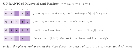
Lemma 5.18 (The ranking of Myrvold and Ruskey). Algorithm 5.9 is a bijection between \([0, N)\) and the \(k\)-permutations of \(n\) items, with RANK its inverse; both take \(O(n + k)\) operations.
Proof. Let \(\pi_j\) be the array before the step \(j\), in UNRANK or in RANK. The step \(l\) moves a value into the position \(n - 1 - l\), and the later steps exchange only positions below it; hence the positions \(n - j, \ldots, n - 1\) of \(\pi_j\) hold \(a_{j-1}, \ldots, a_0\), and the positions \(0, \ldots, n - 1 - j\) hold the other \(n - j\) values. In UNRANK, \(e_j \le n - 1 - j\), and line 6 gives \(a_j = \pi_j[e_j]\), a value not among \(a_0, \ldots, a_{j-1}\): the output is a \(k\)-permutation. In RANK on a \(k\)-permutation \(a\), the array \(\pi_j\) depends only on \(e_0, \ldots, e_{j-1}\), as in UNRANK, and \(a_j\), not among \(a_0, \ldots, a_{j-1}\), lies in a position \(e_j = \pi_j^{-1}[a_j] \le n - 1 - j\); thus the digits are in range, and UNRANK applied to them makes the same exchanges and outputs \(\pi_j[e_j] = a_j\) at each step. Hence \(\mathrm{UNRANK}(\mathrm{RANK}(a)) = a\) for each \(a\), and UNRANK, which maps the \(N\) vectors of digits (in bijection with \([0, N)\) by the mixed radix of lines 4 and 12) onto the \(N\) \(k\)-permutations, is surjective between two sets of the same size, i.e., a bijection whose inverse is RANK. Each step takes \(O(1)\) operations, and line 2 or 9 takes \(O(n)\). \(\square\)
The three rankings thus differ in the order of the ranks and in the
cost. The lexicographic order keeps close abstract states in close
entries, which serves the blocks of Algorithm 5.7 and of the
max-compression; the tree of counters extends it beyond 64 items; the
ranking of Myrvold and Ruskey has no locality, and its cost does not
depend on the digits. The test permutation checks that each ranking is
a bijection, and that LexRanking and TreeRanking enumerate the
\(k\)-permutations in lexicographic order, for \(n = 1, 4, 7\) and every
\(k \le n\), that the two lexicographic rankings agree on 64 items, and
that MyrvoldRuskeyRanking and TreeRanking are inverse on 200 items;
which of the three is fastest in a lookup is a matter of the hardware,
not a theorem. Last, bytes_hash( b , n ) is the hash of the states of
the permutation puzzles, which are arrays of bytes: from the seed
0x9E3779B97F4A7C15 exclusive-or \(n\), it applies the mixing function of
SplitMix64 to the exclusive or of the hash and of each word of 8 bytes of
the array, the last one padded with zeros. It is not injective when \(n >
8\), and the searches need it only as a hash.
5.15 The pattern databases of the permutation puzzles¶
A permutation puzzle has groups of positions, each holding as many
objects as positions, and an object of a group of modulus \(m\) also has
an orientation in \([0, m)\). A move is, for each group, a permutation of
the positions with a turn per position: the object that comes to the
position \(i\) is the one that was at \(\mathrm{from}[i]\), and its
orientation grows by \(\mathrm{turn}[i]\) modulo \(m\). The pancakes, the
burned pancakes (\(m = 2\)), TopSpin, and the corners (\(m = 3\)) and the
edges (\(m = 2\)) of Rubik's cube are such puzzles (Chapter
14); the sliding-tile puzzles are not, since the
effect of a move depends on where the blank is, and they keep the tables
of the previous sections. In the library, PermutationGroup and
PermutationMove describe the groups and the moves, and the concept
PermutationDomain a Domain that is a permutation puzzle:
permutation_groups() and permutation_moves() give the groups and the
moves, every move of the domain being one of them,
permutation_of( s , g , obj , ori ) writes the object at each position
of the group \(g\) in the state \(s\) and its orientation, and
for_each_goal_permutation( g , f ) calls f( obj , ori ) for the group
\(g\) of each goal (of each of them, if they are several).
struct PermutationGroup {
 unsigned size = 0;         ///< the positions, and the objects
 unsigned modulus = 1;      ///< the orientations of an object (1: none)
 bool zero_sum = false;     ///< the orientations sum to 0 modulo modulus
 };

/*- - - - - - - - - - - - - - - - - - - - - - - - - - - - - - - - - - - - -*/
/// a move of a permutation puzzle, by group

struct PermutationMove {
 /// from[ g ][ i ]: the position whose object comes to i
 std::vector< std::vector< std::uint8_t > > from;
 /// turn[ g ][ i ]: what its orientation grows by
 std::vector< std::vector< std::uint8_t > > turn;
 unsigned cost = 1;         ///< the cost, 1 to 254
 };
template< class D >
concept PermutationDomain = Domain< D > &&
 requires( const D & d , const typename D::state_type & s , unsigned g ,
           std::uint8_t * o , std::uint8_t * r ) {
  { d.permutation_groups() }
   -> std::convertible_to< std::vector< PermutationGroup > >;
  { d.permutation_moves() }
   -> std::convertible_to< std::vector< PermutationMove > >;
  d.permutation_of( s , g , o , r );
  d.for_each_goal_permutation( g , detail::permutation_sink{} );
  };
A pattern is a set of \(k\) objects of one group, all the others being "don't care" as in Culberson and Schaeffer [21]: its abstract state is the sequence \(p\) of the positions of its \(k\) objects, a \(k\)-permutation of the \(n\) positions of the group, with their \(k\) orientations \(o\), and its rank is
where \(\mathrm{rank}_R\) is a Ranking and \(k' = k\), or \(k' = k - 1\) when
the pattern holds the whole group and the orientations of the group sum
to 0 modulo \(m\) in every state (PermutationGroup::zero_sum), the last
orientation being then implied by the others. The abstract space has
thus \(N = m^{k'}\, n! / (n - k)!\) states, e.g., the \(8! \cdot 3^7\) of the
corners of Rubik's cube in Korf [59].
PermutationSpace< R > is this space, a model of AbstractSpace: its
goals are the images of the goals of the puzzle, and the predecessor of
\((p, o)\) by a move is the abstract state whose object \(j\) is at
\(\mathrm{from}[p_j]\) with the orientation \(o_j - \mathrm{turn}[p_j]\)
modulo \(m\), the move being skipped when it changes no position and no
orientation of the pattern (it is then a loop of the abstract space). Its
constructor refuses (by std::invalid_argument) a group out of range,
of more than 256 positions or of a modulus of 0 or more than 256, an
empty pattern, an object out of the group or given twice, a move whose
permutation or turns of the group do not have \(n\) entries or whose cost
is not in \(\{1, \ldots, 254\}\), a goal of another size, and a space of
more than \(2^{64}\) states; the ranking refuses, in turn, a group beyond
its limit (64 positions for LexRanking). It does not check that each move permutes the
positions, nor that its turns keep the sum of the orientations when the
last one is implied; these are properties of the puzzle that the
following statement assumes.
Proposition 5.19 (The tables of the patterns
are consistent). Let the moves of a PermutationDomain be permutations
of the positions, each with the cost of the corresponding move of the
domain, and, when the group of a pattern has zero_sum, keep the sum of
the orientations. Then the map \(\psi\) of each state to the abstract state
of a pattern is an abstraction in the sense of Definition
5.1; the table of the pattern built by
Algorithm 5.7, stored in \(B\) bits, is a consistent heuristic; and so is
the maximum of the tables of any set of patterns, and its maximum with
any other consistent heuristic.
Proof. Let a move take the state \(s\) to \(t\). An object \(x\) of the
pattern at the position \(q\) with the orientation \(u\) in \(s\) is, in \(t\),
at the position \(p\) with \(\mathrm{from}[p] = q\) (the move being a
permutation), with the orientation \(o = u + \mathrm{turn}[p]\) modulo
\(m\). Hence \(\psi(s) = (q, u)\) is the predecessor of \(\psi(t) = (p, o)\)
that for_each_predecessor generates for this move, by an edge of the
cost of the move, unless the move changes no position and no orientation
of the pattern, in which case \(\psi(s) = \psi(t)\); with an implied
orientation, the rank uses only the first \(k - 1\) orientations, which
determine the last one in both states. The goals of the puzzle are mapped
to the abstract goals by construction. Hence \(\psi\) satisfies (i) and
(ii) of Definition 5.1, and by Theorem 5.15
the table holds the distances of the abstract space, whose heuristic is
consistent by Proposition 5.2; the
saturation to \(2^B - 1\) keeps it so (Lemma 5.16),
and the maxima are consistent by Lemma 2.5.
\(\square\)
The tables add up only under the condition of §5.6, stated here for any puzzle.
Proposition 5.20 (The sum of the tables). If no move moves (changes the position or the orientation of) objects of two of the patterns, of the same group or of different ones, the sum of their tables is admissible and consistent.
Proof. Let \(P\) be a path from \(s\) to a goal, and \(c_j(P)\) the cost of its moves that move an object of the pattern \(\pi_j\). The image of \(P\) in the abstract space of \(\pi_j\), without its loops, is a path from \(\psi_j(s)\) to an abstract goal of cost \(c_j(P)\), so that the table of \(\pi_j\) is at most \(c_j(P)\); since each move counts in at most one \(c_j(P)\), \(\sum_j c_j(P) \le c(P)\). Along a move \((s, t)\) of cost \(c\), only the abstract state of one pattern may change, by an edge of cost \(c\), and its table changes by at most \(c\) by Proposition 5.19, while the others do not change; at a goal every table is 0. \(\square\)
The condition holds for no puzzle of Chapter 14
but the Towers of Hanoi, whose moves move one disk
(§5.16): a flip of \(k\) pancakes, a turn of
TopSpin and a quarter turn of the cube move several objects, which may
belong to different patterns. In the library, the class template
PermutationPDB< R , B > is the table of one pattern: its constructor
takes the domain, the group, the objects of the pattern, the number of
workers and a cache directory, builds the PermutationSpace from the
domain, and obtains the table by AbstractionTable< B >::cached with
abstract_distances on the workers of an executor
(PermutationPDB.h:389). The key of the file is the
checksum of the groups of the puzzle, of the costs, permutations and turns of
its moves in the group, of the goals of the group, of the group, of the objects
of the pattern, of the name of the ranking and of \(B\). The file is named
perm- followed by the name of the ranking, \(B\) and the key in
hexadecimal, so that two patterns, puzzles or rankings never share a
file, up to the collisions of the checksum. value( loc , ori ) looks up the
abstract state whose object \(x\) is at loc[x] with the orientation
ori[x], and value( d , s ) that of a state of the domain, by
permutation_of. PermutationHeuristic< D , R , B > is the maximum of
several tables, or their sum when additive is true, which the
constructor does not check against Proposition 5.20; it reads the state
once per group and looks up each table of that group. Last,
PDBDomain< D , H > is the domain D with the heuristic \(\max\{h_D(s),
H(s)\}\) for a callable H of the states (such as a PermutationHeuristic
or the HanoiPDB of §5.16): it forwards
the members of D, and OperatorDomain, TreeOperatorDomain,
FeatureDomain, IncrementalFeatureDomain and PerfectHashDomain when
D models them, passes to the expansions of D the heuristic of D
itself (so that an incremental heuristic of D stays right), and
computes H anew for each successor. The declarations are the
following, quoted by hand.
template< Ranking R = LexRanking >
class PermutationSpace {
 public:
 PermutationSpace( const std::vector< PermutationGroup > & groups ,
                   const std::vector< PermutationMove > & moves , unsigned g ,
                   const std::vector< std::uint8_t > & objects ,
                   const std::vector< std::pair< std::vector< std::uint8_t > ,
                                                 std::vector< std::uint8_t >
                                                 > > & goals );
 [[nodiscard]] std::uint64_t size( void ) const noexcept;
 [[nodiscard]] std::uint64_t rank( const std::uint8_t * p ,
                                   const std::uint8_t * o ) const noexcept;
 [[nodiscard]] std::uint64_t rank_objects( const std::uint8_t * loc ,
                                           const std::uint8_t * ori ) const
  noexcept;
 void unrank( std::uint64_t r , std::uint8_t * p , std::uint8_t * o ) const
  noexcept;
 };

template< Ranking R = LexRanking , unsigned B = 8 >
class PermutationPDB {
 public:
 template< PermutationDomain D , WorkerExecutor Executor = ThreadPool >
 PermutationPDB( const D & d , unsigned g ,
                 const std::vector< std::uint8_t > & objects ,
                 unsigned threads = 0 , const std::string & cache = "" ,
                 Executor * = nullptr );
 [[nodiscard]] unsigned value( const std::uint8_t * loc ,
                               const std::uint8_t * ori ) const noexcept;
 template< PermutationDomain D >
 [[nodiscard]] unsigned value( const D & d ,
                               const typename D::state_type & s ) const;
 };

template< PermutationDomain D , Ranking R = LexRanking , unsigned B = 8 >
class PermutationHeuristic {
 public:
 using PDB = PermutationPDB< R , B >;
 PermutationHeuristic( const D & d , std::vector< PDB > pdbs ,
                       bool additive = false );
 [[nodiscard]] unsigned operator()( const typename D::state_type & s ) const;
 };

template< Domain D , class H >
class PDBDomain {
 public:
 PDBDomain( const D & d , const H & h );
 };
The domain and the tables given to PermutationHeuristic and to
PDBDomain must outlive them. A lookup costs permutation_of, i.e.,
\(O(n)\) operations for the group, and, for each table of the group, the
gathering of the \(k\) objects, one rank of §5.14
and one access to the table; the access, to a table of up to tens of
megabytes, is usually the cost that counts.
5.16 The heuristics of the permutation puzzles¶
Each permutation puzzle of Chapter 14 comes with
a heuristic of its own, computed from the state in time linear in its
size, and the tables of §5.15 are combined
with it by PDBDomain; Rubik's cube and the Towers of Hanoi have the
heuristic 0, and their heuristics are the tables alone. In this section
a stack, a ring or a cube is the sequence of its objects by position,
and we prove the properties of each heuristic.
The gaps of the pancakes¶
A stack of \(N\) pancakes of sizes \(0, \ldots, N - 1\) is a permutation
\(p\), \(p[0]\) being the top, and the flip of \(k \ge 2\) reverses \(p[0..k-1]\)
at cost 1; the goal is the identity. A gap is a pair of adjacent
pancakes whose sizes differ by more than one, or the pair of the bottom
pancake and of the plate, of size \(N\), when the bottom pancake is not
\(N - 1\); the gap heuristic of Helmert [60] is
the number of the gaps. In the variant GAP-\(x\) of Holte et al.
[61] the gaps between two pancakes one of
which is among the \(x\) smallest are not counted, while the gap with the
plate always is; it weakens the heuristic in a controlled way, by which
heuristics of graded strength are obtained for the evaluation of the
searches. PancakePuzzle< N > takes \(x\) as the second argument of its
constructor (0 for the gap heuristic itself).
Proposition 5.21 (The gaps). For every \(x \ge 0\), GAP-\(x\) is consistent, 0 at the goal, and the heuristic of the successor by the flip of \(k\) is \(h - \mathrm{gap}(p[k-1], b) + \mathrm{gap}(p[0], b)\), with \(b\) the pancake \(p[k]\) or the plate if \(k = N\); for \(x = 0\) it is 0 only at the goal.
Proof. The flip of \(k\) reverses the block \(p[0..k-1]\), so that the adjacent pairs inside the block are the same unordered pairs after the flip, and the pairs below the block do not change; only the pair at the boundary, \((p[k-1], b)\), becomes \((p[0], b)\), which gives the formula. Whether a pair is a gap depends only on the two sizes as an unordered pair (their difference and the smaller one), except for the plate, which is always the lower element of its pair; hence \(h\) changes by at most 1 along a move of cost 1, and it is consistent. The identity has no gap. Conversely, let \(x = 0\) and let a stack have no gap; then \(p[N - 1] = N - 1\), and if \(p[j] = j\) for each \(j > i\), the pancake \(p[i]\) is one of \(0, \ldots, i\) and differs from \(p[i + 1] = i + 1\) by at most one, i.e., \(p[i] = i\). By induction the stack is the identity. \(\square\)
For \(x > 0\) a stack other than the goal may have no gap that counts,
e.g., \((0, 2, 1, 3, 4, 5, 6)\) under GAP-2, so that GAP-\(x\) is weaker
than GAP-0 by construction (each gap it counts is a gap). In the burned
variant, each pancake also has a side burned, a flip turns every pancake
that it moves, and the goal is the identity with every burned side down.
A pair of adjacent pancakes, \(a\) above \(b\), is good if \(b = a + 1\) and
neither is turned, or if \(a = b + 1\) and both are turned (the pair is
then as after a flip of a block that holds it), and the bottom pancake is
good with the plate if it is \(N - 1\) and not turned; the heuristic of
BurnedPancakePuzzle< N > is the number of the pairs that are not good.
Proposition 5.22 (The burned gaps). The heuristic of the burned pancakes is consistent and 0 exactly at the goal, and the heuristic of the successor by the flip of \(k \ge 1\) is \(h - \mathrm{bad}(p[k-1], b) + \mathrm{bad}(\bar p[0], b)\), with \(\bar p[0]\) the top pancake turned and \(b\) as in Proposition 5.21.
Proof. A flip of \(k\) reverses the block and turns its pancakes; a pair \(a\) above \(b\) inside the block becomes the pair \(\bar b\) above \(\bar a\). If the pair was good with neither turned and \(b = a + 1\), the new pair has both turned and its upper element exceeds the lower by one, so it is good; symmetrically for a good pair with both turned; and a pair with exactly one pancake turned, or whose sizes are not consecutive in the required order, stays bad, since the map of a pair to its image is an involution that preserves the two kinds. Hence only the boundary pair changes, which gives the formula (with \(k = 1\) the flip only turns the top pancake), and the heuristic changes by at most 1 along a move of cost 1; the goal has only good pairs. Conversely, if every pair is good, the bottom pancake is \(N - 1\), not turned, and if the pancakes below the position \(i\) are \(i + 1, \ldots, N - 1\), none turned, the pair of \(p[i]\) and \(i + 1\) is good with \(i + 1\) not turned, so that \(p[i]\) is not turned and equals \(i\); by induction from the bottom the stack is the goal. \(\square\)
The breakpoints of TopSpin¶
A state of TopSpin is a ring of \(N\) tokens, and the move \(i\) reverses the
\(K\) tokens at the positions \(i, \ldots, i + K - 1\) modulo \(N\); the goals
are the \(N\) rotations of the identity. A breakpoint is a pair of
adjacent positions, the position \(N - 1\) being adjacent to 0, whose
tokens are not consecutive modulo \(N\) in either order, and the heuristic
of TopSpin< N , K > is \(\lceil b / 2 \rceil\) for \(b\) breakpoints.
TopSpin is the permutation puzzle of the experiments of Felner et al.
[167] on the dual lookups and of Holte et
al. [30] on the maximum of several
databases, whose tables the library builds by
§5.15.
Proposition 5.23 (The breakpoints). The heuristic \(\lceil b / 2 \rceil\) of TopSpin is consistent and 0 at the goals.
Proof. The move \(i\) reverses the tokens of the turnstile, so that the adjacent pairs inside it are the same unordered pairs after the move, and being consecutive modulo \(N\) in either order is a property of the unordered pair; the pairs outside it do not change. Only the two pairs at the ends of the turnstile, between the positions \(i - 1\) and \(i\) and between \(i + K - 1\) and \(i + K\), may change (when \(K = N\) they are the same pair, whose two tokens are both in the turnstile and simply exchange their positions, so that nothing changes). Hence \(b\) changes by at most 2, and \(\lceil b / 2 \rceil\) by at most 1, along a move of cost 1. A rotation of the identity has the tokens \(t\) and \(t + 1\) modulo \(N\) in adjacent positions, and no breakpoint. \(\square\)
The converse fails: the ring in decreasing order has no breakpoint and is not a goal, so that the heuristic is not 0 exactly at the goals; this does not affect admissibility, which follows from consistency.
The tables of Korf for Rubik's cube¶
RubikPDBHeuristic is the heuristic of Korf
[59]: the maximum of three tables, one of
the 8 corners and two of two sets of 6 of the 12 edges, with 4 bits per
entry, a PermutationHeuristic< RubiksCube , LexRanking , 4 >. The
pattern of the corners is their whole group, whose orientations sum to
0 modulo 3, and its table has \(8! \cdot 3^7 = 88179840\) entries; each
table of edges has \(12! / 6! \cdot 2^6 = 42577920\) entries; the three
take 86667840 bytes, about 83 MiB. The sets of edges are UR, UF, UL, UB, FR, FL and DR,
DF, DL, DB, BL, BR unless given to the constructor, two sets that the
half turn about the axis of the faces L and R maps into each other, so
that their tables have the same distribution of values. The sum of the
tables is not admissible, since a quarter turn moves 4 corners and 4
edges (Proposition 5.20 does not apply), and the heuristic is their
maximum, consistent by Proposition 5.19.
Since the largest values are 11 for the corners and 10 for the edges,
which are below 15, the entries of 4 bits are exact and no saturation
occurs. The test rubik-pdb checks, in an optimized build only (in the
others it only reports that it was skipped), the number of the entries
of each table, its largest value and its mean, 8.764 for the corners and
7.668 for the edges as in [59], within
\(5 \cdot 10^{-4}\); according to the comment of the header, the split into
the first and the last six edges of the order of the positions gives
the means 7.619 and 7.626 instead. The test rubik checks smaller
tables (4 corners and two sets of 4 edges) by IDA\(^*\) and the parallel
IDA\(^*\) against IDA\(^*\) without tables on random walks of 5 moves.
class RubikPDBHeuristic
 : public PermutationHeuristic< RubiksCube , LexRanking , 4 > {
 public:
 explicit RubikPDBHeuristic( const RubiksCube & d , unsigned threads = 0 ,
                             const std::string & cache = "" ,
                             const std::vector< std::uint8_t > & edges_a = {
                              0 , 1 , 2 , 3 , 8 , 9 } ,
                             const std::vector< std::uint8_t > & edges_b = {
                              4 , 5 , 6 , 7 , 10 , 11 } );
 };
The additive tables of the Towers of Hanoi¶
The Towers of Hanoi with four pegs of TowersOfHanoi< D > place \(D\)
disks on the pegs 0 to 3, the peg of the disk \(d\) in the bits \(2d\) and
\(2d + 1\) of a word, and a move takes the top disk of a peg to a peg whose
top disk is larger, or which is empty, at cost 1. The abstraction of the
range of the disks \(l, \ldots, l + k - 1\), HanoiSpace( lo , k , goal ),
keeps only them: its \(4^k\) states are the \(2k\) bits of their pegs (the
rank of the image of a state is a shift and a mask), its goal is the
image of the goal of the puzzle, and its moves are those of the top disks
among the range, each its own inverse, so that the predecessors of a
state are its successors; it admits \(1 \le k \le 16\) and \(l + k \le 32\).
The top disk of each peg is found by hanoi_tops( x , k , top ), which
writes in top[p] the smallest of the \(k\) disks of the word \(x\) on the
peg \(p\), or \(k\) if there is none. Let \(y = x \oplus (p \cdot
\mathtt{0x5555\ldots5})\); a field of two bits of \(x\) equals \(p\) if and
only if both bits of \(y\) in it are 0, i.e., if and only if the bit of
\(\lnot(y \mid (y \gg 1))\) at its low position is 1. A mask keeps the
low bits of the fields of the \(k\) disks, and the disk is the number of
the trailing zeros of the result divided by 2. The disks on a peg being stacked by size,
the smallest one is the top one, and the four pegs take \(O(1)\) operations
on the word each.
Proposition 5.24 (The ranges of disks).
HanoiSpace is an abstraction of TowersOfHanoi in the sense of
Definition 5.1, the table of the range of all
the disks is the exact distance to the goal, and the sum of the tables
of disjoint ranges is admissible and consistent.
Proof. A move of a disk \(d\) of the range from the peg \(a\) to the peg \(b\) requires \(d\) to be the top disk of \(a\) and the top disk of \(b\), if any, to be larger, among all the disks; then the same holds among the disks of the range, and the move is a move of the abstraction, of the same cost. A move of a disk out of the range leaves the image unchanged. The goal is mapped to the abstract goal, which gives Definition 5.1. With the range of all the disks the abstraction is the puzzle itself, and its distances are exact by Theorem 5.15. Each move moves one disk, which belongs to one range at most, and the argument of Proposition 5.20 gives the sum. \(\square\)
HanoiPDB( ks , goal , threads , cache ) is the sum of the tables of the
consecutive ranges of the sizes ks, from the smallest disk, which are
meant to sum to the number of the disks of the puzzle (the constructor
does not check it); each table is an AbstractionTable< 8 >, built by
Algorithm 5.7 or read from the cache directory, where it is named after
the first disk, the size of the range and the rank of the goal, with a
key that mixes the three. The heuristic of Siag et al.
[57] for their instances of 20 disks is the
sum of the tables of the 4 smallest and of the 16 largest disks, i.e., of
\(4^4 = 256\) and \(4^{16} = 2^{32}\) entries, the latter of 4 GiB at a byte
per entry, plus as much during its construction
(§5.13). The test hanoi checks, on the
\(4^8\) states of 8 disks and a random goal, that the table of all the
disks is the exact distance, that the tables of 3 and 5 disks are
admissible and consistent, and A\(^*\) and the parallel IDA\(^*\) with them
on 16 instances.
inline void hanoi_tops( std::uint64_t x , unsigned k , unsigned top[ 4 ] )
 noexcept;

class HanoiSpace {
 public:
 HanoiSpace( unsigned lo , unsigned k , std::uint64_t goal );
 [[nodiscard]] std::uint64_t rank( std::uint64_t s ) const noexcept;
 [[nodiscard]] std::uint64_t size( void ) const noexcept;
 [[nodiscard]] unsigned lo( void ) const noexcept;
 [[nodiscard]] unsigned k( void ) const noexcept;
 };

class HanoiPDB {
 public:
 HanoiPDB( const std::vector< unsigned > & ks , std::uint64_t goal ,
           unsigned threads = 0 , const std::string & cache = "" );
 [[nodiscard]] unsigned operator()( std::uint64_t s ) const noexcept;
 [[nodiscard]] const std::vector< AbstractionTable< 8 > > & tables( void )
  const noexcept;
 };
5.17 Benchmark¶
Our benchmark of the heuristics is the sequential A\(^*\) on the 100
instances of the 15-puzzle of Korf [7], with
the Manhattan distance and with the pattern databases, run by
tools/PDBBench from tools/bench/pdb.sh. First, the
script builds (or loads from its cache directory) the tables of the partitions
5-5-5, 6-6-3 and 7-8, with the blank ignored and, for 5-5-5 and 7-8, minimized;
the searches use the encodings in a nibble, in one bit (without the
reflection), max-compressed (by 16 for 5-5-5, by 8 for 7-8), and by rank
and select when it is available. Then it solves each instance with each
heuristic, twice, running up to JOBS searches at the same time (4 by
default). The costs are integers and exact, i.e., each heuristic is
admissible and each instance is solved to its optimal cost. The machine
and the compiler are those stated in the note of the table. The clock is
the Stopwatch of AStar::solve(), as in
§2.16: it does not include the construction
or the loading of the tables, which precede the search, nor the start of
the process and the reading of the instances.
Table 5.1. A\(^*\) with the Manhattan distance and with the pattern databases on the 100 instances of Korf: for each heuristic (the partition and its encoding), the instances solved, the nodes expanded summed over the instances, and the seconds summed over the instances, each instance the median of its repetitions.
| heuristic | solved | expanded | seconds |
|---|---|---|---|
Placeholder: the results of this table are to be measured on an idle machine and written here by manual/build/tables.py; no number is given until then.
The numbers of expansions do not depend on the machine, and those of the README of the repository (section "Pattern databases", from the same script) are the following, summed over the 100 instances, with the ratio to the Manhattan distance.
| heuristic | blank | entries | memory | expanded | ratio |
|---|---|---|---|---|---|
| Manhattan | 1557138490 | 1 | |||
| 5-5-5, max-compressed by 16 | ignored | min | 49 KB | 681766045 | 2.3 |
| 5-5-5, no reflection | ignored | 1 bit | 197 KB | 369972440 | 4.2 |
| 5-5-5 | ignored | 4 bits | 786 KB | 263234565 | 5.9 |
| 6-6-3 | ignored | 4 bits | 5.8 MB | 167667391 | 9.3 |
| 7-8, no reflection | ignored | 1 bit | 72 MB | 137386424 | 11.3 |
| 7-8, max-compressed by 8 | ignored | min | 36 MB | 119574805 | 13.0 |
| 7-8 | ignored | 4 bits | 288 MB | 43587167 | 35.7 |
| 5-5-5 | minimized | 4 bits | 786 KB | 59968561 | 26.0 |
| 7-8 | minimized | 4 bits | 288 MB | 2019506 | 771 |
The rule of the blank weighs more than the size of the patterns there: with the blank minimized the partition 7-8 expands about 20000 nodes per instance, 21 times fewer than with the blank ignored, at the price of about 6000 reexpansions over the 100 instances. On the 24-puzzle the same script solves with IDA\(^*\) and the partition 6-6-6-6 the ends of 50 random walks of 150 moves of the blank from the goal, with at most \(10^{10}\) expansions each; the README reports 49 of them solved, with optimal costs from 50 to 84, while the 50 instances used by Jinnai and Fukunaga [5] are beyond such a limit.
The tables of §5.13 to
§5.16 are measured by AStarBench on the
permutation puzzles and on the Towers of Hanoi (--domain pancake,
burned, topspin, rubik and hanoi, with the tables of --pdb,
built on --threads workers or read from the directory of --cache),
with the heuristic of the domain alone and with the tables. The clock of
a search does not include the construction of the tables, which is
measured apart, by the same program with an empty cache.
Table 5.2. The pattern databases of the permutation puzzles and of the Towers of Hanoi: for each puzzle, search and heuristic, the instances, the entries and the bytes of the tables, the seconds of their construction, and the instances solved, the nodes expanded and the seconds of the searches, summed over the instances.
| puzzle | search | heuristic | instances | entries | MB | seconds to build | solved | expanded | seconds |
|---|---|---|---|---|---|---|---|---|---|
Placeholder: the results of this table are to be measured on an idle machine and written here by manual/build/tables.py; no number is given until then.
5.18 Notes and references¶
Pattern databases were introduced by Culberson and Schaeffer [21] for the 15-puzzle, with patterns that count each move. Korf and Felner [22] made them additive by counting only the moves of the tiles of the pattern, with the partitions 7-8 and 6-6-6-6 and the reflection, and Felner, Korf and Hanan [23] studied the static and dynamic partitions, among them 5-5-5 and 6-6-3. Yang et al. [28] gave the general theory of the additive abstractions, and Holte et al. [30] showed that the maximum over several smaller databases can beat one larger database. Zahavi et al. [29] introduced the dual lookups, which Felner et al. [31] exploit with the bidirectional pathmax. Felner et al. [24] compressed the tables by the maximum (lossy) and without loss when the merged entries are known to differ by little. Breyer and Korf [25] stored the distances modulo 3, and Clausecker and Reinefeld [27] in one bit with the zero-aware encoding. Samadi et al. [33] learned a smaller model of the entries, and Nagahashi and Takahashi [32] built the largest tables on clusters, by partitioning the ranks among the processes as the blocks of the library are partitioned among the threads. The ranking of Myrvold and Ruskey [34] is the linear-time alternative to the lexicographic one, and the two-bit breadth-first search of Korf [26] is the model of the construction with the blank minimized. The library differs from these works in storing the excess over the Manhattan distance rather than the distance. According to the documentation of the repository, this makes 4 bits per entry enough for the tables of the library, and it keeps the Manhattan distance exact in the max-compression. Yet, the library has neither the dual lookups nor the lossless compression, and the searches that use the tables best on the 24-puzzle, i.e., IDA\(^*\) with the bidirectional pathmax [31], are beyond its IDA\(^*\), which has no pathmax (Chapter 4).
The construction of §5.13 is the algorithm of Dial [65] with the table itself as its buckets; the lexicographic ranking by a tree of counters is that of Bonet [62], and the ranking of Myrvold and Ruskey [34] is restricted to \(k\) items by stopping their unranking after \(k\) steps. The pancake problem is due to Dweighter [63], the gap heuristic to Helmert [60], and its variant GAP-\(x\) to Holte et al. [61]; TopSpin is the permutation puzzle of the experiments of Felner et al. [167] and of Holte et al. [30]. The three tables of Rubik's cube, in half a byte per entry, are those with which Korf [59] solved optimally random instances of the cube, and the additive tables of ranges of disks of the Towers of Hanoi with four pegs follow Felner, Korf and Hanan [23], with the split of Siag et al. [57] for 20 disks. We remark that the permutation puzzles are those on which the dual lookups of [29] and [167] apply most directly, and that the tables of §5.15 have neither the dual lookups nor the compressions of §5.9, whose relative encodings rest on a Manhattan distance that these puzzles do not have.
5.19 Exercises¶
Exercise 5.1 (ctest -R PBeFS.grid). On a grid with 8 moves, where
a move pays the cost of the cell it leaves and \(\sqrt{2}\) times that on
a diagonal, prove that the octile distance times the least cost of a
cell is consistent, that the Euclidean distance times the same cost is
consistent and dominated by it, and that the Manhattan distance is not
admissible (Figure 5.1). The test checks
A\(^*\) with the octile distance against the costs of Dijkstra.
Exercise 5.2 (ctest -R PBeFS.pdb). Compute by hand, by
Algorithm 5.1, the rank of the placement \((2, 7, 1)\) of three tiles on 9
cells, and unrank 229 back to \((4, 0, 7)\) (Figure
5.4). How many ranks does a block of Lemma
5.4 (ii) hold for the pattern of 8 tiles of
the 15-puzzle, and how many blocks does a group of MinNibbleEntries
with \(c = 8\) meet at most? The test checks that unrank and rank are
inverse on every placement of the patterns of the 8-puzzle.
Exercise 5.3 (ctest -R PBeFS.pdb). Prove that with \(k = n - 1\)
tiles (all the tiles in the pattern) both rules of the blank give the
puzzle itself, and deduce from the parity of Chapter
14 that only half of the placements are reachable,
which is why the constructor of TilePattern refuses such a pattern. Give a
placement of a pattern of 2 tiles of the 8-puzzle for which the two
rules give different distances. The test checks the tables of both
rules against a breadth-first search written apart from the library, on
each placement of patterns of 1 to 7 tiles of the 8-puzzle.
Exercise 5.4 (ctest -R PBeFS.pdb). Find a move of the 8-puzzle
along which the sum of the tables of the partition 4-4 with the blank
minimized decreases by more than one, and explain it by the regions of
the blank. Why does the proof of
Theorem 5.8 not apply? The test counts these
moves.
Exercise 5.5 (ctest -R PBeFS.pdb). Prove that the reflection of
Lemma 5.9 is not an automorphism when the
goal has the blank off the diagonal, by an example on the 8-puzzle, and
check that the library then does not use it. Show that
\(\phi(\phi(s)) = s\).
Exercise 5.6 (ctest -R PBeFS.pdb). Prove
Lemma 5.10 for \(M = 4\) with the bit of
ParityBitEntries and the parity of \(m_\pi\), and show by an example
that the residues modulo 2 would not suffice. Why does a relative
encoding with the reflection fail? The test checks that the value of
each state of the 8-puzzle is recovered from the residues only, and
that of each successor from its parent.
Exercise 5.7 (ctest -R PBeFS.pdb). Show by an example that the sum
of the tables of two patterns that share a tile, or of a pattern that
holds the blank, may exceed \(h^*\); the test checks that the library
refuses both.
Exercise 5.8 (ctest -R PBeFS.pdb-search). Show that the
domination of Proposition 5.14 (ii) may be
strict by a placement of the patterns \(\{1\}\) and \(\{2\}\) of the
8-puzzle in which the two tiles block each other. By Theorem
2.15, what can be said of the expansions of
A\(^*\) with the partition 4-4 of the 8-puzzle against those with the
Manhattan distance, and why only below the last layer of \(f\)? The test
checks that they are fewer on its instances.
Exercise 5.9 (ctest -R PBeFS.tiles24). The test builds the
additive database of the 24-puzzle with the 8 patterns of 3 consecutive
tiles, checks that it dominates the Manhattan distance on random walks
of 40 moves, and solves them with IDA\(^*\). Compute the number of the
entries of these tables, and compare it with that of the partition
6-6-6-6 (§5.11).
Exercise 5.10 (ctest -R PBeFS.pdb). Prove that the value of
MinNibbleEntries is admissible, and give two adjacent placements of
the table of Figure 5.5 whose values with
\(c = 2\) differ by 3. The test checks that the max-compressed tables
never exceed the exact ones, that SparseEntries gives the same values
as NibbleEntries, and that a corrupted file is rejected.
Exercise 5.11 (ctest -R PBeFS.abstraction). Run Algorithm 5.7 by
hand on the space of the states \(0, \ldots, n - 1\) with the goal 0 and
the edges between \(r\) and \(r + 1\) of cost \(1 + (r \bmod c)\), for \(c = 2\)
and \(n = 8\): list the layers \(D_k\) and the entries lowered at each of
them. Then show, by Theorem 5.15 (ii), that
the path of 300 states with unit costs is refused, and that so is a
path of 255 states, whose largest distance is 254. The test checks the
distances against the algorithm of Dijkstra on a space of \(10^5\) states
with chords and unreachable states, and the refusal of the path of 300.
Exercise 5.12 (ctest -R PBeFS.abstraction). Prove that the bound
of Theorem 5.15 (iii) on the entries read
is attained, up to a constant, by a ranking that puts the entries of
each distance in every block, and give the bound for a ranking that puts
them in consecutive ranks. Show by an example that the saturation of
Lemma 5.16 may make two adjacent abstract
states, whose distances differ, take the same value. The test checks that
the tables of 4 bits are the tables of 8 bits saturated at 15, their
save and load, the refusal of another key, and that a table of the cache
is built once.
Exercise 5.13 (ctest -R PBeFS.permutation). Unrank 2 by
Algorithm 5.9 with \(n = 4\) and \(k = 2\), compare the result with the
lexicographic rank of the same 2-permutation, and conclude that the
ranks of Myrvold and Ruskey are not in lexicographic order. Then rank
\((4, 0, 7)\) on 9 items by Algorithm 5.8, and check that it gives 229 as
in Figure 5.4. The test checks the three
rankings as bijections for \(n = 1, 4, 7\) and every \(k\), the lexicographic
order of the first two, and the agreement of the lexicographic rankings
on 64 items.
Exercise 5.14 (ctest -R PBeFS.pancake). Prove Proposition
5.21 in detail, and give a stack of 7
pancakes, other than the goal, on which GAP-2 is 0. Is GAP-0 an
abstraction heuristic in the sense of Definition
5.1? The test checks on the 5040 stacks of 7
pancakes that GAP-0 and GAP-2 are consistent and that the domain computes
them incrementally, and A\(^*\) and IDA\(^*\) against the exact distances.
Exercise 5.15 (ctest -R PBeFS.pancake). Compute the number of the
entries of the table of 3 of the 5 burned pancakes, and show that its
abstract space is connected. Then show that the maximum of the gap
heuristic and of a table is consistent, while the sum of the tables of
\(\{0, 1, 2, 3\}\) and of \(\{3, 4, 5, 6\}\) of 7 pancakes (which share an
object) or of \(\{0, 1, 2\}\) and \(\{3, 4, 5\}\) (which do not) may exceed
\(h^*\) (consider the stack in decreasing order), since Proposition
5.20 applies to neither. The test checks
the tables of 4 of 7 pancakes, with two rankings, and of 3 of 5 burned
ones against the exact distances, and the consistency of the maximum.
Exercise 5.16 (ctest -R PBeFS.topspin). Prove Proposition
5.23, and show that the ring in decreasing
order has no breakpoint; is it reachable in TopSpin with 8 tokens and a
turnstile of 4? Explain why the table of a pattern of TopSpin is built
from the \(N\) goals at once, and what its value would be if only the
identity were a goal. The test checks the breakpoints and a table of 5
tokens on the 40320 rings of TopSpin with 8 tokens, and A\(^*\) and IDA\(^*\)
with them.
Exercise 5.17 (ctest -R PBeFS.rubik-pdb). Derive the numbers of
the entries of the three tables of Korf, and show by the state after one
quarter turn from the goal that the sum of the table of the corners and
of a table of the edges is not admissible. Why does the half turn about
the axis of L and R give the two tables of the edges the same mean? The
test checks the sizes, the largest values and the means of the tables
against [59], in an optimized build.
Exercise 5.18 (ctest -R PBeFS.hanoi). Prove that hanoi_tops
returns the top disk of each peg, and Proposition
5.24. Show that the sum of the tables of two
ranges of disks that are not consecutive (e.g., the disks 0 and 2 in one
table and 1 in the other) is still admissible. The test checks, on the
\(4^8\) states of 8 disks, that the table of all the disks is exact and
that the tables of 3 and 5 disks are additive and consistent.