2. Best-first search and A*¶
[Source: include/PBeFS/astar/AStar.h (AStar, astar),
include/PBeFS/astar/Node.h (Node, trace_path),
include/PBeFS/astar/Solution.h (Solution, SearchStats,
SearchOptions, Status), include/PBeFS/astar/Domain.h
(OperatorDomain, for_each_child),
include/PBeFS/astar/ExplicitGraph.h;
include/PBeFS/astar/GreedySearch.h (GreedySearch,
GreedyOptions, GreedyNode, GreedyOpen, HeuristicCache,
QueueSpec, gbfs),
include/PBeFS/astar/EnforcedHillClimbing.h
(EnforcedHillClimbing, EHCOptions, ehc),
include/PBeFS/astar/IteratedSearch.h
(IteratedSearch, IteratedOptions, lama_phases),
include/PBeFS/astar/WidthSearch.h (NoveltyTable,
IteratedWidth, SerializedWidth, BestFirstWidth, WidthOptions,
iw, siw, bfws, features_of, added_features); the tests astar,
grid, graph, limits and reopen of test/test.cpp, and
gbfs, gbfs-queues, ehc, iterated, width and planning]
We are concerned in this chapter with the sequential best-first search
of the graph of a Domain (cf. Chapter 1,
whose notation we use throughout), and in particular with A\(^*\)
[9], on which the other searches of the
library are built. We first describe the generic best-first search, the
difference between a search of the tree of the paths and a search of the
graph, and the priorities that give breadth-first search, depth-first
search, the algorithm of Dijkstra and A\(^*\). Then we state A\(^*\) as the
library implements it, and we prove its correctness under an admissible
heuristic and its stronger properties under a consistent one. The last
sections discuss the reopening of the closed nodes, the breaking of the
ties, the pruning of the move back to the parent and the counters by
which a search is measured. The data structures of OPEN and CLOSED, with
the cost of their operations, are the subject of Chapter
3, and we only point to them here. Also,
the searches that hold less than CLOSED in memory (IDA\(^*\) and the
search with delayed duplicate detection on the disk) are those of
Chapter 4, and the heuristics themselves
are those of Chapter 5.
The second part of the chapter, from §2.11 to §2.15, first gives the goal test at the generation of a state, by which A\(^*\) saves the expansions of its last layer while keeping its guarantees (§2.11). It then turns to the searches that give up the optimality of the path for speed, as the satisficing planners do: greedy best-first search with the OPEN lists of the planners (§2.12), enforced hill-climbing (§2.13), the iterated searches of LAMA (§2.14) and the width-based searches (§2.15); the parallel greedy searches are those of Chapter 12. The benchmark, the notes and the exercises of both parts close the chapter (§2.16 to §2.18).
Throughout the chapter we assume that the costs of the edges are nonnegative, \(c(u, v) \ge 0\), and that the heuristic is nonnegative, \(h(u) \ge 0\), as it is in all the domains of the library. The second assumption is used only to have \(h(t) \le h^*(t) = 0\) imply \(h(t) = 0\) at a goal \(t\) (a heuristic that is positive at a goal may make A\(^*\) return a path that is not optimal, cf. Exercise 2.6).
2.1 Searching a tree and searching a graph¶
A best-first search keeps the nodes it knows in two sets: OPEN, the frontier, i.e., the nodes generated but still unexpanded, and CLOSED, the nodes already expanded. At each iteration it removes from OPEN a node of least priority \(f(u)\), tests whether it is a goal and, if it is not, expands it, i.e., generates its successors by the domain (which are then generated) and puts them in OPEN. A state is thus, at any time, in one of three conditions: not generated yet, generated and waiting in OPEN, or expanded and in CLOSED (the faint, light and darker states of the figures of this chapter).
In its simplest form, a search of this kind does not look at what it has already seen: each successor is put in OPEN as a new node, even if its state has been generated before. Such a search explores the tree of the paths from \(s_0\), in which a state typically appears many times, once for each path that reaches it, and it is called a tree search. Figure 2.1 shows a graph in which two paths reach \(c\), and the tree that a tree search explores on it: \(c\) and \(t\) appear twice, and so does everything below them. On a graph with many short cycles, e.g., a grid, the paths of length \(d\) are exponentially many in \(d\), while the states within distance \(d\) are only polynomially many, and a tree search may even fail to terminate on a finite graph, since a cycle gives paths of any length (cf. section 3.1 of [10]).
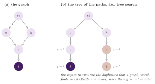
A graph search keeps, instead, one node per state: it looks each
successor up among the states already generated (the duplicate
detection), and it drops the successor if its state is known with a \(g\)
that is not larger. This needs CLOSED to be a dictionary of the
generated states, and the library keeps one (the NodeTable of Chapter
3), but it bounds the nodes by the states.
One case remains: a successor \(v\) whose state is known, but which has
now been reached through a cheaper path. If \(v\) is still in OPEN, its
\(g\) is lowered and its priority with it; if \(v\) has already been
expanded, it is reopened, i.e., moved from CLOSED back to OPEN with
the new \(g\), so that the cheaper path is propagated to its successors
when \(v\) is expanded again. Whether a search must reopen depends on the
priority and, for A\(^*\), on the heuristic (see
§2.6 and §2.7).
Dropping a duplicate without comparing the values of \(g\) is safe only
when the first copy of a state is known to be reached through a path of
least cost, e.g., in a breadth-first search with unit costs, or when an
optimal path is not required.
Algorithm 2.1 (best-first graph search with a priority \(f\)).
 1  procedure BEST-FIRST(s₀, f)
 2     CLOSED ← {s₀}, with g(s₀) ← 0 and parent(s₀) ← nil
 3     OPEN ← {s₀}
 4     while OPEN ≠ ∅ do
 5        u ← a node of OPEN of least f(u); remove it from OPEN
 6        if u is a goal then return the path to u, of cost g(u)
 7        mark u as expanded
 8        for each successor v of u do
 9           g' ← g(u) + c(u, v)
10           if v ∉ CLOSED then         ▷ a new state
11              add v to CLOSED, with g(v) ← g' and parent(v) ← u
12              put v in OPEN
13           else if g' < g(v) then     ▷ a cheaper path to v
14              g(v) ← g';  parent(v) ← u
15              put v in OPEN, whether it was expanded or not
16     return unsolvable
As in the library, CLOSED holds all the generated states, each with a
flag that records whether it has been expanded (line 7); the closed list
of the textbooks is the subset of CLOSED with the flag set, and OPEN is
a queue of the others. At line 6 the path is rebuilt by following the
pointers parent from the goal back to \(s_0\) (the function trace_path
of Node.h:168). Note that the goal test is done when a node is
selected at line 5, rather than when it is generated at line 10. In
fact, a goal generated through a path of cost \(g\) is not necessarily
reached optimally, since a node of OPEN of smaller priority may still
lead to a cheaper one; only the test at the selection gives the
guarantee of Theorem 2.9.
2.2 The priority¶
Algorithm 2.1 is a family of searches, one for each priority \(f\); the classical ones are the following, with \(d(u)\) the number of edges of the path found to \(u\) (cf. chapter 3 of [13] and chapter 2 of [10]).
- Breadth-first search (BrFS), \(f(u) = d(u)\), with the ties broken first in, first out: the nodes are expanded by layers of depth, and the first goal selected is one with the fewest edges, which is optimal when all the costs are equal.
- Depth-first search (DFS), \(f(u) = -d(u)\), with the ties broken last in, first out: the search follows one path as deep as it goes and backtracks only at a dead end; OPEN then behaves as a stack, and the recursive formulation does without it altogether, keeping only the current path (which is the basis of the memory-bounded searches of Chapter 4).
- The algorithm of Dijkstra, also called uniform-cost search, \(f(u) = g(u)\): the nodes are expanded by nondecreasing cost from \(s_0\), and the first goal selected is optimal for any nonnegative costs.
- A\(^*\), \(f(u) = g(u) + h(u)\), with \(h\) the heuristic of the domain: \(f(u)\) estimates the cost of a solution through \(u\), and with an admissible \(h\) the first goal selected is optimal (§2.5). With \(h = 0\), A\(^*\) is the algorithm of Dijkstra.
- Greedy best-first search, \(f(u) = h(u)\), which goes towards the goal that looks closest and is not optimal in general, and weighted A\(^*\), \(f(u) = g(u) + w\,h(u)\) with \(w \ge 1\), which returns a path of cost at most \(w\,C^*\) when \(h\) is admissible.
For a graph with branching factor \(b\) (the largest number of successors of a state), an optimal solution of \(d\) edges and cost \(C^*\) (the optimal cost of Table 1.2 of §1.4), costs of at least \(\varepsilon > 0\), and largest depth \(m\) of a state, the first four have the following properties, the time and the space being measured in nodes generated.
| search | complete | optimal | time and space |
|---|---|---|---|
| breadth-first | finite \(b\) | equal costs | \(O(b^{d+1})\) |
| depth-first, graph | finite graphs | no | \(O(b^{m})\) |
| Dijkstra | finite \(b\), \(c\ge\varepsilon\) | yes | \(O(b^{1+D})\) |
| A\(^*\) | as Dijkstra | \(h\) admissible | see the text |
Here \(D = \lfloor C^* / \varepsilon \rfloor\), and the cost of A\(^*\) is Proposition 2.19. The rows of breadth-first search and of the algorithm of Dijkstra are Proposition 2.20, which derives them from the theorems on A\(^*\) with \(h = 0\); the bound of breadth-first search has the exponent \(d + 1\) because the goal is tested when it is selected (with the test at the generation, as in section 3.4 of [13], it would be \(d\)). The row of the depth-first search of a graph, which the library does not implement, is taken from section 3.4 of [13]: it terminates on a finite graph since it expands each state at most once, and it is not optimal since it returns the first goal that it reaches, whatever the cost of its path.
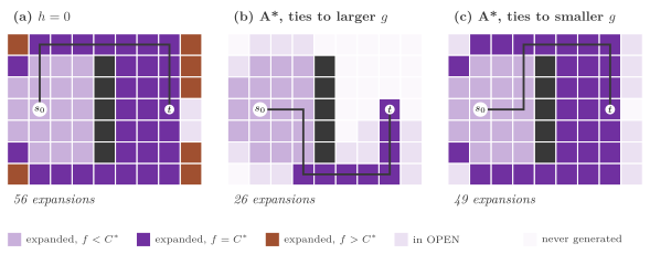
With a consistent heuristic, the nodes expanded by A\(^*\) are a subset of those expanded by the algorithm of Dijkstra, but for the ties of the last layer: by Theorem 2.14, A\(^*\) expands only nodes with \(g^*(u) + h(u) \le C^*\), hence with \(g^*(u) \le C^*\), while the algorithm of Dijkstra expands all those with \(g^*(u) < C^*\) (Theorem 2.15 with \(h_1 = 0\) gives the same conclusion when \(h\) is positive on the states that are not goals). Note that the depth-first search of a tree needs only \(O(b\,m)\) memory, the current path and the siblings of its nodes, which is the reason for its use in Chapter 4; the depth-first search of a graph keeps CLOSED and needs as much memory as the states it visits. Consider the graph of five states \(s_0, a, b, c, t\) drawn in Figure 2.2, whose seven edges \((s_0, a)\), \((s_0, b)\), \((a, b)\), \((a, c)\), \((b, c)\), \((b, t)\) and \((c, t)\) carry their costs and whose optimal path \(s_0, a, b, c, t\) costs 7 (the figure is read in §2.3). Breadth-first search expands \(s_0, a, b, c\) and \(t\) and returns the path \(s_0, b, t\) of two edges and cost 10; depth-first search (with the successors pushed in the order \(a, b\)) expands \(s_0, b, t\) and returns the same path; the algorithm of Dijkstra and A\(^*\) both expand \(s_0, a, b, c, t\) and return the optimal path. That A\(^*\) expands no fewer nodes than Dijkstra there is due to the size of the example. On the grid of Figure 2.6, a map of \(9 \times 7\) cells with 4 moves of unit cost and a wall between \(s_0\) and \(t\) (the figure is read in §2.6), a run of Algorithm 2.2 with \(h = 0\) and the ties broken first in, first out expands 56 cells, while A\(^*\) with the Manhattan distance and the ties broken in favor of the larger \(g\), and last in, first out among equal \(f\) and \(g\) (the rule of the bucket queue of the library), expands 26 of them. These counts come from a separate simulation of Algorithm 2.2 with these rules of the ties, not from a run of the library, whose heap breaks the ties among equal \(f\) and \(g\) in no fixed order.
Of these searches, the library implements A\(^*\) (AStar.h), and
gets the algorithm of Dijkstra from it with a domain whose heuristic is
zero. A wrapper of a Domain that returns 0 from heuristic and passes
0 as the heuristic of each successor is all that one needs, and the
tests use one (Blind, test/test.h:346) to check A\(^*\) on
the grids against the costs of Dijkstra (test grid). On a domain with unit
costs the same wrapper gives a breadth-first search, up to the order of the
ties within a layer. The breadth-first search is also a search of its own,
BreadthFirst, with the baselines of
§4.14; greedy best-first search is
GreedySearch (§2.12), and weighted A\(^*\) is
AStar with the weight of SearchOptions, the subject of
Chapter 6 (a wrapper of the domain whose
heuristic is \(w\,h\) gives it too, cf.
Exercise 2.7).
Status — planned. The library has no depth-first search of a graph as a search of its own. The depth-first searches of a tree are those of Chapter 4.
2.3 A* in the library¶
The interface¶
A search of the library takes a type D that models the concept Domain of
Domain.h:169. Such a type has the type state_type (a
copyable value compared with ==), the arithmetic type cost_type of \(g\), \(h\)
and the costs, and the members initial_state(), is_goal( s ),
heuristic( s ), hash( s ) (a well spread 64-bit hash, used by CLOSED) and
for_each_successor( s , h_s , f ). The last one calls f( t , c , h_t ) for
each successor \(t\) of \(s\), with \(c = c(s, t)\) and \(h_t = h(t)\); the value
\(h(s)\) is passed in, and hence the domain can compute \(h(t)\) incrementally, as
the sliding-tile puzzles do with the Manhattan distance (cf. Chapter
1 and Chapter 14).
The class template AStar< D , Open > (AStar.h:153) is
constructed from the domain, which must outlive it, and from the
SearchOptions of Solution.h:188. These are node_limit,
the number of stored nodes at which the search gives up and returns
Status::node_limit (0, the default, for no limit; Proposition
2.17 states when the test is made), and
expected_nodes, the number of nodes that CLOSED is sized for at the start,
instead of growing by doublings as it fills (0, the default, for a small
initial table). Then solve() runs the search and returns a Solution
(Solution.h:153), i.e., the Status (solved,
unsolvable or node_limit), the cost of the path, the path itself as the
sequence of its states from \(s_0\) to the goal (empty unless the status is
solved), and the counters stats of §2.10;
solved() tells whether the status is solved. The OPEN list Open defaults
to the bucket queue (BucketOpenList) for integer costs and to the heap
(HeapOpenList) otherwise. The function astar( domain , open , options )
(AStar.h:326) chooses it at run time by an OpenKind, i.e.,
automatic (the default of the class), heap or buckets; for a domain whose
costs are not integers it runs the heap whatever the OpenKind, since the
bucket queue needs integer keys. Both lists are described in Chapter
3. Their declarations are the following (quoted by
hand, since in the header they come with their bodies).
template< Domain D , class Open = /* buckets if cost_t< D > is integral,
                                     else the heap */ >
class AStar {
 public:
 explicit AStar( const D & domain , const SearchOptions & options = {} );
 [[nodiscard]] Solution< state_t< D > , cost_t< D > > solve( void ) const;
 };

template< Domain D >
[[nodiscard]] Solution< state_t< D > , cost_t< D > >
astar( const D & domain , OpenKind open = OpenKind::automatic ,
       const SearchOptions & options = {} );
The following example, from the test case manual of the library
(ctest -R PBeFS.manual), solves an instance of the 8-puzzle with the
Manhattan distance by both lists, and then with a node limit.
const EightPuzzle d( EightPuzzle::parse( "7 2 4 5 0 6 8 3 1" ) );
SearchOptions o;
o.expected_nodes = 1 << 12;                // CLOSED sized at the start
const auto s = astar( d , OpenKind::automatic , o );   // the buckets
const auto t = astar( d , OpenKind::heap , o );        // the heap
// the path goes from the initial state to a goal, one move per cost unit
const bool path = s.solved() && ( s.status == Status::solved ) &&
                  ( s.path.front() == d.initial_state() ) &&
                  d.is_goal( s.path.back() ) &&
                  ( s.path.size() == std::size_t( s.cost ) + 1 );
const auto & st = s.stats;      // expanded, reexpanded, generated,
                                // duplicates and stored
o.node_limit = 5;               // stop after storing 5 nodes
const auto l = astar( d , OpenKind::automatic , o );
// l.status == Status::node_limit, and l.path is empty
The examples of the repository (examples/) do the same on all the
domains of the library.
The algorithm¶
In the library, the search is Algorithm 1 of the survey of Fukunaga et
al. [1], i.e., Algorithm 2.1 with \(f(u) =
g(u) + h(u)\). Two choices on the data structures change its form, while
its outcome stays the same. First, OPEN holds entries \((f, g, u)\)
rather than nodes, ordered by increasing \(f\) and, for equal \(f\), by
decreasing \(g\) (§2.8). Second, neither OPEN
list of the library can lower the key of an entry: a node reached
through a cheaper path is pushed again with its new \(g\), and the old
entry, which records the \(g\) of its push, becomes stale, i.e., its
node is closed or has a different \(g\). A stale entry is dropped when it
reaches the top of OPEN. We give the pseudocode of the Doxygen comment
of AStar.h.
Algorithm 2.2 (A\(^*\)).
 1  procedure A*(s₀)
 2     CLOSED ← {s₀}, with g(s₀) ← 0 and parent(s₀) ← nil
 3     OPEN ← {(f(s₀), g(s₀), s₀)}
 4     while OPEN ≠ ∅ do
 5        (f, g, u) ← the first entry of OPEN; remove it from OPEN
 6        if u is closed or g ≠ g(u) then continue      ▷ a stale entry
 7        close u
 8        if u is a goal then return the path to u, of cost g(u)
 9        for each successor v of u do
10           g' ← g(u) + c(u, v)
11           if v ∉ CLOSED then
12              add v to CLOSED, with g(v) ← g' and parent(v) ← u
13              push (g' + h(v), g', v) in OPEN
14           else if g' < g(v) then           ▷ a cheaper path: reopen v
15              g(v) ← g';  parent(v) ← u;  v is not closed
16              push (g' + h(v), g', v) in OPEN
17     return unsolvable
We now comment on the lines that are not obvious. Line 6 drops the stale
entries. An entry whose node is closed was pushed before the node was
expanded with a smaller (or equal) \(g\), and an entry whose \(g\) differs
from that of the node was overtaken by a cheaper path, whose entry is in
OPEN with a smaller \(f\). In fact, the flag closed of line 7 records
that the node has been expanded with its current \(g\); line 15 clears
it when a cheaper path is found, whether the node was waiting in OPEN or
already expanded, which is the reopening of
§2.7. Also, the node keeps a second flag,
expanded, which is never cleared and by which the expansions of a node
already expanded are counted (Node.h:82). With a consistent
heuristic the branch at lines 14 to 16 is taken only for nodes still in OPEN
(Theorem 2.13).
Algorithm 2.2 leaves out, as all the pseudocode of the book
(§1.4), the counters, the node limit and
the prefetches. Since the claims of §2.10
are about the counters, we also give the loop of AStar::solve()
(AStar.h:180) with all of them. Its expansion is split in two
passes: the first asks the domain for all the successors of \(u\), computes the
hash of each one and prefetches, i.e., asks the processor to start
loading into its cache, the slot of CLOSED where the lookup of that
successor will start; the second does the lookups, whose cache misses
thus overlap instead of being paid one after the other
(§3.8).
Algorithm 2.3 (A\(^*\) as AStar::solve() runs it, with a node
limit \(L\), \(L = 0\) meaning none).
 1  procedure SOLVE(s₀, L)
 2     CLOSED ← {s₀}, with g(s₀) ← 0, h(s₀) and parent(s₀) ← nil
 3     OPEN ← {(h(s₀), 0, s₀)}
 4     while OPEN ≠ ∅ do
 5        (f, g, u) ← the first entry of OPEN; remove it from OPEN
 6        if u is closed or g ≠ g(u) then continue      ▷ a stale entry
 7        close u;  expanded ← expanded + 1
 8        if u was expanded before then reexpanded ← reexpanded + 1
 9        mark u as expanded
10        if u is a goal then return (solved, g(u), the path to u)
11        K ← ∅                              ▷ pass 1: the successors
12        for each (v, c(u, v), h(v), o) of CHILDREN(u, h(u), op(u)) do
13           compute the hash of v and prefetch its slot of CLOSED
14           append (v, c(u, v), h(v), o) to K
15        generated ← generated + |K|
16        for each (v, c, h(v), o) of K, in order do  ▷ pass 2: lookups
17           g' ← g(u) + c
18           if v ∉ CLOSED then
19              add v to CLOSED, with g(v) ← g', parent(v) ← u, op(v) ← o
20              push (g' + h(v), g', v) in OPEN
21           else if g' < g(v) then
22              g(v) ← g';  parent(v) ← u;  op(v) ← o;  v is not closed
23              push (g' + h(v), g', v) in OPEN
24           else duplicates ← duplicates + 1
25        if L > 0 and |CLOSED| ≥ L then return (node_limit)
26     return (unsolvable)
Here CHILDREN is Algorithm 1.1 of §1.4, which
passes the operator \(o\) of each successor and skips the move back to the
parent in a domain that knows its operators
(§2.9); op(u) is the operator stored in the
node, no_op for \(s_0\). Line 19 is the lookup and the insertion of CLOSED
(find_or_insert of NodeTable, which builds the node only when the state is
new), and stored is \(|\)CLOSED\(|\) when the search ends, since CLOSED keeps
one node per state. Also, line 7 sets the flag closed and line 9 the flag
expanded of Node.h:81 and Node.h:82; the path
of line 10 is rebuilt by trace_path (Node.h:168).
Proposition 2.17 proves that Algorithm 2.3 does what Algorithm 2.2 does, and what the node limit changes.
A trace¶
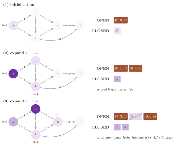
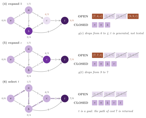
Figure 2.2 and Figure 2.3 follow Algorithm 2.2 on a graph of five states with a consistent heuristic (the values \(g/h\) are written next to each state, in rust where they change, and the entries of OPEN are listed in the order of the queue, the new ones in rust and the stale ones struck out). In step (3) the expansion of \(a\) finds a path to \(b\) of cost 3, cheaper than the edge of cost 4 from \(s_0\): \(b\) is still in OPEN, and the entry \((8, 4, b)\) becomes stale. In step (4) the goal \(t\) is generated with \(g = 9\), but it is not tested, and in step (5) the expansion of \(c\) lowers its \(g\) to 7; in step (6) \(t\) is selected and the path \(s_0, a, b, c, t\) of cost 7 is returned, while three stale entries are still in OPEN and are never popped.
2.4 Admissible and consistent heuristics¶
Much of the behavior of A\(^*\) depends on two properties of \(h\), which we now define (the heuristics of the library and how they are obtained are discussed in Chapter 5). Let \(h^*(u)\) be the least cost of a path from \(u\) to a goal (\(+\infty\) if there is none), and \(k(u, v)\) the least cost of a path from \(u\) to \(v\) (\(+\infty\) if there is none).
Definition 2.1 (Admissible heuristic). A heuristic \(h\) is admissible if \(h(u) \le h^*(u)\) for each state \(u\).
Definition 2.2 (Consistent heuristic). A heuristic \(h\) is consistent if \(h(t) = 0\) for each goal \(t\) and \(h(u) \le c(u, v) + h(v)\) for each edge \((u, v)\).
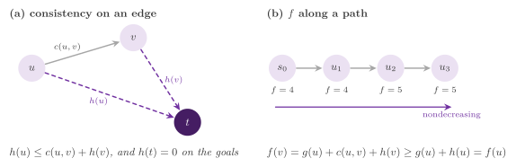
The inequality of Definition 2.2 is the triangle inequality of \(h\) along the edges (Figure 2.4): the estimate from \(u\) is never larger than the cost of an edge plus the estimate from its head. Some textbooks define consistency over all the pairs of states, with \(k(u, v)\) in place of \(c(u, v)\), and call the edgewise property monotonicity; the two are equivalent, as the next lemma shows, and the property of \(f\) along a path that is sometimes also called monotonicity is a consequence of either (Lemma 2.12).
Lemma 2.3 (Edgewise and pairwise consistency). A heuristic satisfies \(h(u) \le c(u, v) + h(v)\) for each edge \((u, v)\) if and only if it satisfies \(h(u) \le k(u, v) + h(v)\) for each pair of states \(u, v\).
Proof. Since \(k(u, v) \le c(u, v)\) for each edge, the pairwise inequality implies the edgewise one. Conversely, if \(v\) is not reachable from \(u\), then \(k(u, v) = +\infty\) and there is nothing to prove; otherwise, let \(u = w_0, w_1, \ldots, w_q = v\) be a path of least cost. Summing the edgewise inequalities \(h(w_{i-1}) - h(w_i) \le c(w_{i-1}, w_i)\) for \(i = 1, \ldots, q\), the left-hand side telescopes to \(h(u) - h(v)\) and the right-hand side is \(k(u, v)\). \(\square\)
Lemma 2.4 (Consistency implies admissibility). A consistent heuristic is admissible.
Proof. If no goal is reachable from \(u\), then \(h^*(u) = +\infty\). Otherwise, let \(t\) be a goal with \(k(u, t) = h^*(u)\); by Lemma 2.3, \(h(u) \le k(u, t) + h(t) = h^*(u)\), since \(h(t) = 0\). \(\square\)
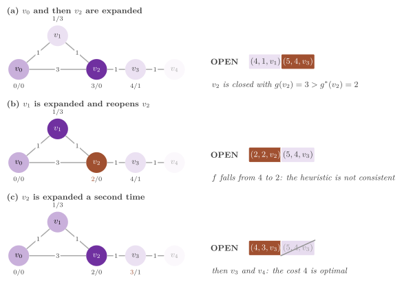
Of course, the converse does not hold. On the graph of
Figure 2.7, whose states \(v_0, \ldots, v_4\)
are joined by the arcs \((v_0, v_1)\), \((v_1, v_2)\), \((v_2, v_3)\) and
\((v_3, v_4)\) of cost 1 and by the arc \((v_0, v_2)\) of cost 3, each
directed from the state of the smaller index to that of the larger one
(the figure draws them as lines), with \(s_0 = v_0\) and the goal \(v_4\) (the
figure is read in §2.7), the heuristic
\(h = (0, 3, 0, 1, 0)\) is admissible, since \(h^* = (4, 3, 2, 1, 0)\), but
\(h(v_1) = 3 > c(v_1, v_2) + h(v_2) = 1\). The sequence score of Nilsson
(SequenceScore.h, used by the example 8Puzzle) is a
heuristic of the sliding-tile puzzles that is not even admissible: A\(^*\) then
usually expands fewer nodes, but it may return a path that is not
optimal (SequenceScore.h:50).
Both properties are preserved by the maximum of heuristics, which is used by the pattern databases of Chapter 5 (the maximum with the reflection of a table) and in general to combine several heuristics of a domain.
Lemma 2.5 (The maximum of heuristics). Let \(h_1, \ldots, h_m\) be heuristics and \(h(u) = \max_i h_i(u)\). If all the \(h_i\) are admissible, so is \(h\); if all are consistent, so is \(h\).
Proof. The first claim is immediate, since \(h_i(u) \le h^*(u)\) for each \(i\). For the second, \(h(t) = \max_i h_i(t) = 0\) at a goal; for an edge \((u, v)\), let \(i\) be an index with \(h(u) = h_i(u)\): then \(h(u) = h_i(u) \le c(u, v) + h_i(v) \le c(u, v) + h(v)\). \(\square\)
We say that a heuristic \(h_2\) is more informed than \(h_1\) if \(h_2(u) > h_1(u)\) for each state \(u\) that is not a goal; Theorem 2.15 below shows that, between two consistent heuristics, the more informed one never makes A\(^*\) expand a node that the other does not expand.
2.5 The correctness of A*¶
We now prove that A\(^*\) with an admissible heuristic returns an optimal path, and that it terminates. Our argument rests on one invariant on OPEN (cf. Lemma 1 of [9] and section 2.1 of [1]), which we state for any state \(w\) (a goal being a special case), since §2.6 needs it in that form. Let \(g^*(w)\) be the least cost of a path from \(s_0\) to \(w\), and recall that \(C^* = h^*(s_0)\).
Lemma 2.6 (Values of \(g\)). At any time of Algorithm 2.2, \(g(u)\) is the cost of a path from \(s_0\) to \(u\), and hence \(g(u) \ge g^*(u)\), for each node \(u\) in CLOSED.
Proof. By induction on the assignments to \(g\): \(g(s_0) = 0\) is the cost of the empty path, and lines 12 and 15 set \(g(v) = g(u) + c(u, v)\), the cost of the path to \(u\) of value \(g(u)\) followed by the edge \((u, v)\). \(\square\)
Lemma 2.7 (The invariant of OPEN). Let \(w\) be a state reachable from \(s_0\) that, at the start of an iteration of the loop at line 4, is not closed with \(g(w) = g^*(w)\). Then each path of least cost \(P\) from \(s_0\) to \(w\) has a node \(u\) that is not closed, has \(g(u) = g^*(u)\) and has in OPEN the entry \((g^*(u) + h(u), g^*(u), u)\), which is not stale.
Proof. Let \(u\) be the first node of \(P\) that is not closed with its optimal \(g\); it exists, since \(w\) is such a node. If \(u = s_0\), then \(s_0\) has not been expanded yet, and it is in OPEN with \(g = 0\) by line 3. Otherwise the predecessor \(p\) of \(u\) on \(P\) is closed with \(g(p) = g^*(p)\); since the prefix of \(P\) to \(u\) is a path of least cost, \(g^*(u) = g^*(p) + c(p, u)\). When \(p\) was last expanded, with \(g(p) = g^*(p)\), line 10 computed \(g' = g^*(u)\) for \(u\). Then either \(u\) was new, or it had \(g(u) > g'\), or it already had \(g(u) \le g' = g^*(u)\). In the first two cases lines 12 to 16 set \(g(u) = g^*(u)\) and pushed the entry \((g^*(u) + h(u), g^*(u), u)\), while in the third case \(g(u) = g^*(u)\) by Lemma 2.6 and such an entry had been pushed when \(g(u)\) took that value. Since \(g(u)\) cannot fall below \(g^*(u)\), it has not changed since then, and by the choice of \(u\) the node has not been closed with it; hence the entry is still in OPEN, and it is valid. \(\square\)
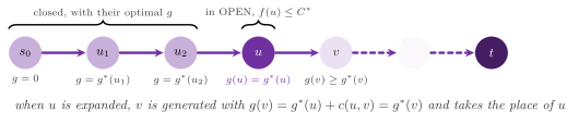
In other words (Figure 2.5), the expanded prefix of an optimal path is followed by one node of OPEN that carries its optimal \(g\). Its expansion generates the next node of the path with its optimal \(g\), which takes its place. Note that the proof needs the reopening of lines 14 to 16: the next node might have been closed before with a larger \(g\), and without the reopening it would never be put back in OPEN.
Lemma 2.8 (Every selected node has \(f \le C^*\)). If \(h\) is admissible and a goal is reachable from \(s_0\), each entry \((f, g, u)\) that is selected at line 5 and is not stale, before a goal is returned, has \(f \le C^*\), and therefore \(g^*(u) + h(u) \le C^*\).
Proof. Let \(t^*\) be a goal with \(g^*(t^*) = C^*\). Before the search returns, \(t^*\) is not closed with \(g(t^*) = C^*\) (closing it would end the search at line 8), and by Lemma 2.7 an optimal path to \(t^*\) has a node \(u'\) with an entry of key \(f' = g^*(u') + h(u') \le g^*(u') + h^*(u') = C^*\) in OPEN, the inequality being the admissibility of \(h\) and the equality the optimality of the path through \(u'\). The entry selected at line 5 has the least key in OPEN, and hence \(f \le f' \le C^*\); finally, \(g^*(u) + h(u) \le g(u) + h(u) = f\) by Lemma 2.6, since a selected entry that is not stale has \(g = g(u)\). \(\square\)
Theorem 2.9 (Admissibility of A\(^*\)). If \(h\) is admissible and A\(^*\) returns a path, the path is optimal, i.e., its cost is \(C^*\).
Proof. Let the search return at line 8 with the goal \(t\) selected from a non-stale entry \((f, g(t), t)\). Since \(h(t) \le h^*(t) = 0\) and \(h \ge 0\), \(h(t) = 0\) and \(f = g(t)\); by Lemma 2.8, \(g(t) \le C^*\), and by Lemma 2.6, \(g(t)\) is the cost of a path from \(s_0\) to \(t\), and therefore \(g(t) \ge C^*\). \(\square\)
It remains to prove that A\(^*\) terminates. On a finite graph this holds for any heuristic, admissible or not; on an infinite graph it needs a positive lower bound on the costs, and the absence of cycles of nonpositive cost is not enough.
Lemma 2.10 (The parent pointers form a tree).
At any time of Algorithm 2.2, the pointers parent of the nodes of
CLOSED form a tree rooted at \(s_0\), and
\(g(\mathrm{parent}(v)) + c(\mathrm{parent}(v), v) \le g(v)\) for each
node \(v \ne s_0\).
Proof. The inequality holds when parent(v) is set, with equality, and is
preserved afterwards, since \(g\) never increases and a later change of
parent(v) sets it again. Suppose that the pointers form a cycle
\(v_1, \ldots, v_q\), with \(v_{i-1}\) the parent of \(v_i\) (indices modulo \(q\)),
and let \(v_j\) be the node of the cycle whose pointer was set last, at line 15,
to \(u = v_{j-1}\). Just before that assignment the other pointers of the cycle
were already in place, and the inequality along the path
\(v_j, v_{j+1}, \ldots, v_{j-1} = u\) gives \(g(u) \ge g(v_j)\), the costs being
nonnegative; the new value \(g(u) + c(u, v_j)\) is then not smaller than the old
\(g(v_j)\), while line 14 requires it to be strictly smaller. Hence there is no
cycle, and since each node but \(s_0\) has a parent, the pointers form a tree
rooted at \(s_0\). \(\square\)
Theorem 2.11 (Termination of A\(^*\)). Algorithm 2.2 terminates (i) on any finite graph, and (ii) on any graph with finite branching whose costs are at least some \(\varepsilon > 0\), provided that \(h\) is admissible and that a goal is reachable from \(s_0\).
Proof. Each iteration either drops a stale entry or closes a node, and the entries are pushed only by lines 3, 13 and 16, once per value taken by \(g\) of a node. Hence, it suffices to show that the pairs \((v, g(v))\) taken by the nodes are finitely many. (i) By Lemma 2.6, each value of \(g(v)\) is the cost of a path from \(s_0\) to \(v\), and the successive values of \(g(v)\) are strictly decreasing. A path decomposes into a simple path and a multiset of simple cycles, whose costs are nonnegative. Since the simple paths and the simple cycles of a finite graph are finitely many, there is an \(\eta > 0\) not larger than the cost of each simple cycle of positive cost, and a path whose cost is at most the first value of \(g(v)\) contains at most that value over \(\eta\) cycles of positive cost. Thus the costs of such paths are finitely many, and so are the values of \(g(v)\). (ii) By Lemma 2.8, each node \(u\) expanded before the end has \(g(u) \le f \le C^*\); by Lemma 2.10, \(g(u)\) is at least the cost of the path of the tree from \(s_0\) to \(u\), which therefore has at most \(C^* / \varepsilon\) edges. Under a finite branching, the paths of at most \(C^* / \varepsilon\) edges are finitely many, and so are the nodes that may be expanded and their successors. The values of \(g\) are then finitely many by (i), applied to the finite subgraph that these nodes span. \(\square\)
We remark that the condition of (ii) cannot be weakened to the absence
of cycles of nonpositive cost. On an infinite chain \(s_0, w_1, w_2,
\ldots\) whose \(i\)-th edge costs \(2^{-i}\), with a goal reached from \(s_0\)
by one edge of cost 1 and \(h = 0\), each node of the chain has \(g < 1\)
and is selected before the goal, and the search never ends. On a finite
graph without a reachable goal, A\(^*\) ends with OPEN empty and returns
Status::unsolvable, which the test limits checks on a grid split by
a wall; on an infinite graph it may end only by the node limit.
2.6 Consistent heuristics¶
With a consistent heuristic A\(^*\) has stronger properties, which we now prove. The values of \(f\) do not decrease along a path, and the nodes are selected by nondecreasing \(f\); each node is closed with its optimal \(g\) and never reopened; and the set of the expanded nodes is determined by \(C^*\), up to the ties on the last value of \(f\).
Lemma 2.12 (Monotonicity of \(f\)). If \(h\) is consistent and \(v\) is a successor of \(u\) with \(g(v) = g(u) + c(u, v)\), then \(f(v) \ge f(u)\).
Proof. \(f(v) = g(u) + c(u, v) + h(v) \ge g(u) + h(u) = f(u)\), by Definition 2.2. \(\square\)
Theorem 2.13 (No reopening). If \(h\) is consistent, each node is closed by Algorithm 2.2 with \(g(u) = g^*(u)\); hence no closed node is ever reopened, each state is expanded at most once, and the keys of the selected non-stale entries are nondecreasing.
Proof. Suppose that a node \(u\) is selected from a non-stale entry with \(g(u) > g^*(u)\). By Lemma 2.7 applied to \(w = u\), an optimal path to \(u\) has a node \(w'\) with an entry of key \(g^*(w') + h(w')\) in OPEN, and \(w' \ne u\), since \(g(u) \ne g^*(u)\). Now, by Lemma 2.3, \(h(w') \le k(w', u) + h(u)\), and \(g^*(w') + k(w', u) = g^*(u)\) since \(w'\) is on an optimal path to \(u\); hence \(g^*(w') + h(w') \le g^*(u) + h(u) < g(u) + h(u)\). Thus the entry of \(w'\) has a smaller key than that of \(u\), and \(u\) would not have been selected. Each node is therefore closed with its optimal \(g\), which no path can improve, and line 14 never holds for a closed node; a state is then expanded only when its node is closed, i.e., once. Finally, when \(u\) is expanded with key \(f(u)\), all the keys in OPEN are at least \(f(u)\), and by Lemma 2.12 so are the keys pushed by the expansion; hence the next selected key is not smaller. \(\square\)
Thus, the keys of the selected entries grow by layers of equal \(f\), and \(C^*\) is the last layer. Equivalently, A\(^*\) is the algorithm of Dijkstra on the reduced costs \(c'(u, v) = c(u, v) - h(u) + h(v)\), which consistency makes nonnegative. Indeed, along any path \(s_0 = w_0, \ldots, w_q = u\) the reduced costs telescope to \(\sum_i c(w_{i-1}, w_i) + h(u) - h(s_0)\): the reduced cost of a path is its cost plus \(h(u) - h(s_0)\), which depends only on its ends, the least reduced cost from \(s_0\) to \(u\) is \(g^*(u) + h(u) - h(s_0)\), and the key \(g(u) + h(u)\) of A\(^*\) is the key of the algorithm of Dijkstra on \(c'\) plus the constant \(h(s_0)\), which orders the entries in the same way. The next two results characterize the nodes that A\(^*\) expands (Figure 2.6); the first part holds for any admissible heuristic and is Lemma 2.8 again.
Theorem 2.14 (Necessary and sufficient conditions of expansion). Let \(h\) be admissible and a goal be reachable. (i) Every node \(u\) expanded by Algorithm 2.2 before the goal it returns has \(g^*(u) + h(u) \le C^*\). (ii) If \(h\) is consistent, each node \(u\) with \(g^*(u) + h(u) < C^*\) is expanded before the search returns.
Proof. (i) is Lemma 2.8. (ii) Suppose that the search returns, selecting a goal \(t\) with key \(C^*\) (by Theorem 2.9), while \(u\) has not been expanded. By Lemma 2.7, an optimal path to \(u\) then has a node \(w\) with an entry of key \(g^*(w) + h(w)\) in OPEN. As in the proof of Theorem 2.13, this key is at most \(g^*(u) + h(u) < C^*\), and \(t\), of key \(C^*\), would not have been selected before it. \(\square\)
A\(^*\) with a consistent heuristic thus expands all the nodes with \(f^*(u) = g^*(u) + h(u) < C^*\), none with \(f^*(u) > C^*\), and some of those with \(f^*(u) = C^*\), which ones depending on the order of the ties (§2.8). The comparison of two heuristics follows.
Theorem 2.15 (A more informed heuristic expands no more nodes). Let \(h_1\) and \(h_2\) be consistent, and \(h_2\) more informed than \(h_1\). Every node expanded by A\(^*\) with \(h_2\), but the goal it returns, is expanded by A\(^*\) with \(h_1\).
Proof. Let \(u\) be a node that is not a goal and is expanded with \(h_2\). By Theorem 2.14 (i), \(g^*(u) + h_2(u) \le C^*\), and since \(h_1(u) < h_2(u)\), \(g^*(u) + h_1(u) < C^*\); by Theorem 2.14 (ii), \(u\) is expanded with \(h_1\). \(\square\)
If \(h_2\) only dominates \(h_1\), i.e., \(h_2(u) \ge h_1(u)\), the same argument covers the nodes with \(g^*(u) + h_2(u) < C^*\), and the nodes of the last layer may differ by the ties (cf. section 2.1 of [1]). Theorem 2 of [9] also shows that A\(^*\) is optimal, in the number of expanded nodes, among the admissible searches that use the same information; the precise sense of that claim, which depends on the ties, is discussed in chapter 2 of [10].
2.7 Reopening with an inconsistent heuristic¶
When \(h\) is admissible but not consistent, Theorem
2.13 fails: a node may be closed with a \(g\)
larger than \(g^*\), and it is then reopened when a cheaper path to it is
found, as line 14 of Algorithm 2.2 allows. Figure
2.7 shows the graph of the test reopen
(test/files.cpp:623), in which \(h(v_1) = 3\) makes \(v_1\) look
expensive. After \(v_0\), A\(^*\) expands \(v_2\) (key 3) with \(g(v_2) = 3\), through
the edge of cost 3, and then \(v_1\) (key 4), which finds the path of cost 2
to \(v_2\) and reopens it. Then \(v_2\) is expanded a second time with key
2, smaller than the key 4 of the previous expansion (the keys of the
selected entries are thus not monotone), and the search returns the path
\(v_0, v_1, v_2, v_3, v_4\) of cost 4, which is optimal, as Theorem
2.9 guarantees. The test checks the cost and
that the counter reexpanded is positive.
Reopening keeps A\(^*\) optimal, but it may cost a great deal: with an
inconsistent heuristic the number of expansions may grow much faster
than the number of states; a family of graphs on which it grows
exponentially in the number of states is discussed in chapter 2 of
[10], and we do not reproduce it here. The
analysis of Felner et al.
[31] discusses when inconsistent heuristics
are nevertheless useful. In the library a domain does not declare
whether its heuristic is consistent, and AStar always reopens. The
counter reexpanded of the SearchStats reports how many expansions
were of nodes already expanded; it is zero when the heuristic is
consistent (by Theorem 2.13), and it is the
first quantity to look at when a search is slower than expected (cf.
Chapter 5). The pattern databases with the
blank minimized, for instance, are admissible but not consistent, and
A\(^*\) reopens nodes on them. Note that a search that cannot reopen,
such as the search with delayed duplicate detection of Chapter
4, refuses a successor whose \(f\) is smaller
than that of its parent.
2.8 The ties within the last layer¶
Theorem 2.14 leaves free the order of the
nodes with the same \(f\). This order matters on the domains with few
distinct values of \(f\), where the last layer \(f = C^*\) may hold a large
part of the nodes generated. Both OPEN lists of the library break the
ties in favor of the larger \(g\), i.e., of the node with the smaller \(h\),
which is closer to a goal if the heuristic is informative. That on the
domains with unit costs the search then usually reaches a goal after
expanding a small part of the last layer is an empirical observation,
made in the experiments of Burns et al. [4],
and not a theorem: an adversarial order of the successors can make
either rule expand the whole layer. On the grid of Figure
2.6, the simulation of
§2.2 expands 26 cells with the ties in favor
of the larger \(g\), against 49 with the ties in favor of the smaller one;
the difference is entirely in the layer \(f^* = C^*\) (8 of its 31 cells
against all of them), as Theorem 2.14
requires. Among the entries with the same \(f\) and \(g\), the bucket queue
takes the last one pushed, which tends to follow one path down the
layer, while the heap takes any. Also, the library can be built with one
of three sets of data structures, i.e., three implementations of OPEN,
CLOSED and the arena of the nodes chosen at compile time
(Structures.h, §3.12); they
break these last ties differently, and hence they may expand different nodes of
the last layer, while by Theorem 2.14 they expand
the same nodes below it when \(h\) is consistent.
2.9 Pruning the move back to the parent¶
On a domain whose moves are reversible at the same cost, such as the
sliding-tile puzzles and the grids with symmetric costs, each expansion
generates the parent of the node it expands. Such a successor is a duplicate
that CLOSED would drop, since it is reached with a \(g\) larger than that of the
parent; but detecting it costs a hash and a lookup, i.e., one of the about \(b\)
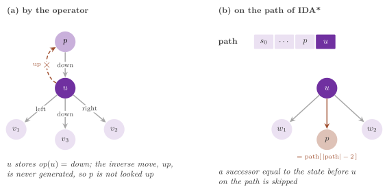
lookups of each expansion. A domain that models the concept OperatorDomain
(Domain.h:356) avoids it: its
for_each_successor( s , h_s , op , f ) receives the operator op that
generated \(s\) (no_op at the root), skips the successor that the inverse of
op leads to, and passes to f the operator of each successor it generates,
which the node stores in its field op (Figure
2.8, left). The function for_each_child
(Domain.h:705) calls this form when the domain has it and the
plain one otherwise, and all the searches of the library go through it.
Proposition 2.16 (Parent pruning changes no
outcome). If the inverse of each operator has the same cost, skipping
the successor that the inverse of the operator of \(u\) leads to changes
neither the path returned by Algorithm 2.2 nor the order of its
expansions; it changes only the counters generated and duplicates
of §2.10, each by the number of the
successors skipped.
Proof. Let \(p = \mathrm{parent}(u)\) be the state skipped, so that \(g(u) \ge g(p) + c(p, u)\) by Lemma 2.10. The skipped successor would have \(g' = g(u) + c(u, p) \ge g(p) + 2\,c(p, u) \ge g(p)\), and \(p\) is in CLOSED; hence line 14 would not hold, and the successor would only be counted as a duplicate, without any push. \(\square\)
A search that keeps no CLOSED, such as IDA\(^*\), cannot detect the duplicate at all, and without the pruning it would walk back and forth along each edge; on a domain without operators it compares each successor with the state two places back on its path (Figure 2.8, right, and Chapter 4). The pruning by operator and its use in the fast implementations of A\(^*\) are discussed by Burns et al. [4].
2.10 The cost of a search and its counters¶
The SearchStats of a Solution (Solution.h:73) report
what a search did. For AStar the counters are the following, written by the
lines of Algorithm 2.3 given in parentheses.
expanded, the expansions, the reexpansions included (line 7; an iteration that drops a stale entry is not an expansion);reexpanded, the expansions of nodes already expanded before (line 8, §2.7);generated, the successors generated, after the parent pruning (line 15);duplicates, the successors whose state was already in CLOSED with a \(g\) not larger, and which were dropped (line 24);stored, the distinct nodes stored at the end, i.e., the states generated and the root, which measure the memory;seconds, the wall-clock time ofsolve(), from its first line to its return (§2.16).
The other fields of SearchStats are for the parallel searches: sent
and messages count the nodes and the batches of nodes sent to another
worker, and expanded_by and stored_by hold the expansions and the
nodes of each worker, from which load_balance() and
communication_overhead() compute the load balance and the
communication overhead (Chapter 8 and
Chapter 9). For AStar, sent and
messages are 0, and the two vectors have the single entries
expanded and stored. We first prove that Algorithm 2.3, from which
these counters are read, is Algorithm 2.2, and then the relations
between them.
Proposition 2.17 (Algorithm 2.3 is Algorithm
2.2). Let both algorithms run with the same OPEN list and the domain
enumerate the successors of each state in the same order. (i) With
\(L = 0\), Algorithm 2.3 pops the same entries, closes the same nodes in
the same order and returns the same status, cost and path as Algorithm
2.2. (ii) With \(L > 0\), it does the same until the first expansion after
which \(|\mathrm{CLOSED}| \ge L\), and then returns node_limit; at that
moment \(L \le |\mathrm{CLOSED}| \le \max(L - 1, 1) + b\), with \(b\) the
largest number of successors of a state, and a goal that is selected is
always returned, since the test of line 10 precedes that of line 25.
Proof. (i) The counters and the hashes are written but never read by the search, and a prefetch changes the content of the cache, not that of CLOSED or of OPEN. Pass 1 calls only the domain, which reads neither list; hence \(K\) is the sequence of the successors that Algorithm 2.2 visits at its line 9, in the same order. During pass 2, \(g(u)\) does not change: an improvement of \(u\) through one of its own successors would need \(g(u) + c(u, u) < g(u)\), i.e., a negative cost. Thus each iteration of lines 16 to 24 does, on the same CLOSED, what lines 10 to 16 of Algorithm 2.2 do for the same successor (a state that occurs twice in \(K\) is found at its second occurrence where the first left it, in both algorithms). Lines 19 and 22 also store the operator, which only CHILDREN reads, and it reads it to skip a successor that Algorithm 2.2 would treat as a duplicate (Proposition 2.16). By induction on the iterations, the two algorithms go through the same states of CLOSED and OPEN. (ii) The test of line 25 is made only after an expansion, and before it the two algorithms agree by (i). When the search stops, either the last expansion was the first one, made with \(|\mathrm{CLOSED}| = 1\), or the test failed after the expansion before it, with \(|\mathrm{CLOSED}| \le L - 1\), the iterations that drop a stale entry adding no node; and an expansion adds at most \(b\) nodes. \(\square\)
Note that a search that stops at the limit may have found no goal only
because it stopped, and also that a search whose OPEN would have become
empty at the same iteration returns node_limit rather than
unsolvable.
Proposition 2.18 (The counters of A\(^*\)). Let
\(I\) be the number of the improvements of \(g\) at line 22 of Algorithm
2.3. When solve() returns, (i) generated \(=\) (stored \(- 1\)) \(+ I
+\) duplicates; (ii) the entries pushed in OPEN are stored \(+ I\), at
most \(I\) of them are dropped as stale, and the iterations of the loop at
line 4 are at most stored \(+ I\); (iii) expanded \(-\) reexpanded is
the number of the distinct states expanded, which is at most stored;
(iv) if \(h\) is consistent, reexpanded \(= 0\) and the \(I\) improvements
are all of nodes in OPEN.
Proof. (i) Each element of \(K\) goes through exactly one of the branches of lines 18, 21 and 24; the first adds a node to CLOSED, which starts with \(s_0\) and never loses a node, the second is an improvement and the third a duplicate. (ii) The entries are pushed by lines 3, 20 and 23, i.e., \(1 + (\mathtt{stored} - 1) + I\) times. Let \(v\) be a node improved \(I_v\) times, so that it has \(1 + I_v\) entries, pushed with strictly decreasing values of \(g\) (line 21); call latest the entry pushed last at a given time, the only one whose \(g\) equals \(g(v)\). The flag closed of \(v\) is set only by the pop of its latest entry (line 7, after the test of line 6), and it is cleared by each later push (line 22); hence the latest entry is never popped while \(v\) is closed, and its pop is not stale. A stale pop of \(v\) is thus the pop of an entry that is no longer the latest, and there are at most \(I_v\) of these, since the last entry pushed is always the latest. Summing over the nodes, at most \(I\) entries are stale; each iteration pops one entry, and an entry is popped once. (iii) Line 7 counts each expansion and line 8 those of the nodes whose flag expanded, never cleared, was already set; their difference is the number of the nodes on which the flag is set, i.e., of the states expanded at least once, which are in CLOSED. (iv) By Theorem 2.13, no closed node is reopened, i.e., line 21 holds only for nodes that are not closed, and each state is expanded at most once. \(\square\)
For instance, a search whose initial state is a goal returns at line
10 of its first iteration, with expanded \(= 1\), generated \(= 0\)
and stored \(= 1\), a path of one state and the cost 0 (the edge cases
checked by check_astar_edges, test/test.h:474). From the
counters one can derive the effective branching factor
generated / expanded, the fraction of the successors that are duplicates and
the rate of expansions per second; the number \(I\) of the improvements is not
counted on its own, but it follows from (i).
The time of a best-first search is thus the number of its expansions
times the time of an expansion, which is made of (i) the extraction of
an entry from OPEN, (ii) the generation of the successors by the
domain, (iii) the evaluation of their heuristic, (iv) the duplicate
detection in CLOSED and (v) the insertions in CLOSED and OPEN. We state
the cost of AStar with the costs of the data structures of Chapter
3 as parameters.
Proposition 2.19 (The cost of A\(^*\)). Let
\(X\), \(\Gamma\) and \(N\) be the values of expanded, generated and
stored at the end of a search, \(I\) the improvements, \(b\) the largest
number of successors of a state and \(t_D\) a bound on the time that the
domain takes to generate one successor, with its heuristic and its hash.
Then Algorithm 2.3 takes time
with \(t_{\mathrm{look}}\), \(t_{\mathrm{push}}\) and \(t_{\mathrm{pop}}\) the times of a lookup or insertion of CLOSED and of a push and a pop of OPEN, and the last term the rebuilding of the path; it holds \(N\) nodes, at most \(N + I\) entries of OPEN, the slots of CLOSED and \(b\) successors at a time. In particular: (i) with the heap of \(d = 4\) children (Proposition 3.3) the term of OPEN is \(O((N + I) \log (N + I))\); (ii) with the bucket queue, integer costs and a consistent \(h\) (Proposition 3.5, under its hypotheses) it is \(O(N + I + f_{\max})\), with \(f_{\max}\) the largest key pushed; (iii) with uniform hashing and the load factor of CLOSED at most \(7/10\) (Proposition 3.11) the expected value of \(t_{\mathrm{look}}\) is \(O(1)\), amortized over the doublings; (iv) if \(h\) is consistent and a goal is reachable, \(I \le \Gamma\), \(X\) is at most the number of the states \(u\) with \(g^*(u) + h(u) \le C^*\), and \(N \le 1 + \Gamma \le 1 + b\,X\).
Proof. Each iteration of the loop pops one entry, and those that are
not stale run lines 7 to 25 once. Lines 11 to 15 call the domain once
per successor, i.e., \(\Gamma\) times overall, besides an \(O(1)\) work per
expansion; lines 16 to 24 make one lookup per successor and one push per
new node or improvement; the pops are at most the pushes, which are \(N +
I\) by Proposition 2.18 (ii); and the path
of line 10 has at most \(N\) states, since the pointers parent form a
tree on CLOSED (Lemma 2.10). The memory
follows in the same way, the entries in OPEN at any time being at most
those pushed. Then (i), (ii) and (iii) are the propositions quoted. For
(iv), \(I \le \Gamma\) by Proposition 2.18
(i); by Theorem 2.13 each state is expanded
at most once, and by Theorem 2.14 (i) only
if \(g^*(u) + h(u) \le C^*\); finally, \(N - 1 \le \Gamma \le b\,X\) by
Proposition 2.18 (i). \(\square\)
On the sliding-tile puzzles and on the grids, \(t_D\) is a few instructions (the Manhattan distance of a successor is that of its parent plus or minus one), and the time goes mostly to the data structures, i.e., to \(t_{\mathrm{look}}\), \(t_{\mathrm{push}}\) and \(t_{\mathrm{pop}}\); with a costly heuristic, such as a pattern database whose tables do not fit in the cache, \(t_D\) may dominate instead (Chapter 5). Also, A\(^*\) stores every state that it generates, i.e., \(N \ge X\); whether a search runs out of memory before it runs out of time depends on the domain and on the machine, and it is not a property that the bounds above decide.
The uninformed searches of §2.2 are A\(^*\) with \(h = 0\), and their properties follow from the results of this chapter.
Proposition 2.20 (The uninformed searches). Let \(h = 0\), so that Algorithm 2.2 is the algorithm of Dijkstra, and the costs be nonnegative. (i) If it returns a path, the path is optimal; it terminates on a finite graph, and on a graph of finite branching with costs at least \(\varepsilon > 0\) and a reachable goal. (ii) In the latter case it expands each state at most once, only states with \(g^*(u) \le C^*\), and at most \(\sum_{i = 0}^{D} b^i\) of them, \(D = \lfloor C^* / \varepsilon \rfloor\); it thus generates and stores \(O(b^{1 + D})\) nodes. (iii) With unit costs, the key \(g(u)\) of a node selected from a non-stale entry is the least number of edges of a path from \(s_0\) to \(u\), the search is a breadth-first search up to the order of the ties among the nodes of equal depth, and it generates and stores \(O(b^{d + 1})\) nodes, with \(d = C^*\) the number of edges of an optimal path.
Proof. The heuristic \(h = 0\) is consistent (Definition 2.2: \(0 \le
c(u, v) + 0\), and 0 at the goals), hence admissible by Lemma
2.4. (i) is Theorem
2.9 and Theorem
2.11. (ii) By Theorem
2.13 each state is expanded at most once,
with \(g(u) = g^*(u)\), and by Theorem 2.14
(i) only if \(g^*(u) \le C^*\). By Lemma 2.10
the path of the tree of the pointers parent from \(s_0\) to \(u\) costs at
most \(g(u) \le C^*\), and since each of its edges costs at least
\(\varepsilon\) it has at most \(D\) edges. A node has at most \(b\) children
in that tree, so that the nodes at depth \(i\) of the tree are at most
\(b^i\); the expanded ones are thus at most \(\sum_{i \le D} b^i\), each
generates at most \(b\) successors, and the stored nodes are at most one
more than the successors generated (Proposition
2.18 (i)). (iii) With unit costs, \(g^*(u)\)
is the least number of edges of a path to \(u\), which is the key of \(u\)
when it is selected (by Theorem 2.13), and
the keys selected are nondecreasing: the nodes are expanded by layers of
depth, which is breadth-first search up to the order within a layer.
The bound is (ii) with \(\varepsilon = 1\) and \(C^* = d\). \(\square\)
2.11 The goal test at generation¶
Algorithm 2.2 tests the goal when a node is selected, which makes the
first goal selected an optimal one; a goal generated earlier, at the
expansion of its parent, waits in OPEN until no node of smaller \(f\) is
left. The option goal_at_generation of SearchOptions (off by
default) lets AStar keep the best goal generated so far and stop as soon
as OPEN can no longer improve it, which saves the expansions of the
nodes of \(f = C^*\) that come before a goal in the order of the ties, and
all of the last layer of \(f\) when the parent of an optimal goal has a
smaller \(f\) (e.g., with the blind heuristic and positive costs, the case of
the planning tasks of Chapter 16). Thus the search
keeps the incumbent \(\hat u\), the goal of least \(g\) among those that it
has generated with \(h = 0\), and precedes line 5 of Algorithm 2.2 with the
line 4' of the Doxygen comment of AStar.h.
Algorithm 2.4 (The line 4' of A\(^*\) with the goal test at generation; the stale entries at the top of OPEN are dropped before the test).
We update the incumbent after each successor \(v\) that lines 11 to 16
put in OPEN, i.e., that is new or reached through a cheaper path: if
\(h(v) = 0\), \(v\) is a goal and \(\hat u\) does not exist or has \(g(\hat u) >
g(v)\), then \(\hat u \leftarrow v\), and the counter goals_generated of
SearchStats counts these updates. Since a goal has \(h = 0\) under an
admissible heuristic, each goal generated is a candidate; with an
inadmissible heuristic a goal of positive \(h\) is never the incumbent, and
it is still found by line 8. This test is made only on a successor with \(h
= 0\), so that a domain whose heuristic is informative pays a single
comparison per successor, and the goal test of line 8 is kept: a goal
selected there also ends the search. Also, the incumbent is a node of
CLOSED, and a later improvement of its \(g\) (the node reached by a cheaper
path, lines 14 to 16) lowers \(g(\hat u)\) with it. With a weight \(w\) of the
heuristic (Chapter 6), the keys of OPEN
are \(f' = g + w h\), and line 4' compares the least key with \(g(\hat u)\)
on the scale of the keys (the method live of Weight).
Theorem 2.21 (The goal test at generation keeps the guarantees). Let \(h\) be admissible and a goal be reachable. Then Algorithm 2.2 with line 4' returns a path of cost \(C^*\); with the priority \(f' = g + w h\), \(w \ge 1\), it returns a path of cost at most \(w C^*\).
Proof. If the search returns at line 8, the claim is Theorem 2.9 (and, with the weight, the bound of Exercise 2.7), since line 4' only adds a way of returning, and it changes neither OPEN nor CLOSED otherwise: the stale entries that it drops are those that line 6 would drop. Let the search return at line 4' with the incumbent \(\hat u\). Since \(g(\hat u)\) is the cost of a path from \(s_0\) to the goal \(\hat u\) (Lemma 2.6), \(g(\hat u) \ge C^*\), and it suffices to prove \(g(\hat u) \le C^*\). Let \(t^*\) be a goal with \(g^*(t^*) = C^*\). At the start of the iteration \(t^*\) is not closed with \(g(t^*) = C^*\), since closing it would have ended the search at line 8; by Lemma 2.7, an optimal path to \(t^*\) has a node \(u'\) whose entry \((g^*(u') + h(u'), g^*(u'), u')\) is in OPEN and is not stale. Its key is at most \(g^*(u') + h^*(u') = C^*\), by admissibility, and line 4' returns only if no live entry has a key smaller than \(g(\hat u)\); hence \(g(\hat u) \le g^*(u') + h(u') \le C^*\). With the priority \(f'\), the key of the entry of \(u'\) is \(g^*(u') + w h(u') \le w (g^*(u') + h^*(u')) = w C^*\), and the same argument gives \(g(\hat u) \le w C^*\). \(\square\)
The proof needs the reopening of lines 14 to 16 through Lemma 2.7, as that of Theorem 2.9 does, and it does not need a consistent heuristic. Next, we state what the test saves, and that it never costs an expansion.
Proposition 2.22 (The expansions with the goal test at generation). Let both searches run on the same domain with the same OPEN list. (i) The sequence of the nodes expanded by Algorithm 2.2 with line 4' is a prefix of that of Algorithm 2.2 without it. (ii) If \(h\) is consistent, \(s_0\) is not a goal, and some optimal path from \(s_0\) to a goal \(t\) has \(g^*(p) + h(p) < C^*\) at the predecessor \(p\) of \(t\), the search with line 4' expands exactly the nodes \(u\) with \(g^*(u) + h(u) < C^*\), each once.
Proof. (i) Line 4' reads OPEN and drops only stale entries, which the search without it drops at line 6 without expanding anything; the incumbent is written but not read by lines 5 to 16. Hence the two searches pop the same live entries in the same order until the first one returns, and the one with line 4' returns either at the same time (line 8) or earlier (line 4'). (ii) By Theorem 2.13, the keys of the selected entries are nondecreasing and each node is closed with its optimal \(g\), and by Theorem 2.14 (ii), each node of \(g^* + h < C^*\) is expanded; hence all of them are expanded before any node of key at least \(C^*\), \(p\) among them, with \(g(p) = g^*(p)\). The expansion of \(p\) generates \(t\) with \(g = g^*(p) + c(p, t) = C^*\), and \(h(t) = 0\); thus, when the first entry of key at least \(C^*\) reaches the top of OPEN, the incumbent exists and has \(g(\hat u) = C^*\) (it cannot be smaller, by Theorem 2.21), and line 4' returns. Each node expanded before has key, i.e., \(g^* + h\), smaller than \(C^*\), and is expanded once by Theorem 2.13. \(\square\)
Without line 4', A\(^*\) also expands the nodes of \(f = C^*\) that precede
the first goal in the order of the ties, i.e., between none and all of
them (§2.8); with the blind heuristic and
unit costs these are the states at distance \(C^*\) from \(s_0\), the last
and usually the largest layer of the breadth-first search. We remark that
the hypothesis on \(p\) of (ii) fails when the optimal goals are reached
only
from nodes of \(f = C^*\), e.g., with the perfect heuristic \(h = h^*\),
where every node of an optimal path has \(f = C^*\); then line 4' saves
only the ties that come after the incumbent. On the planning tasks of the
library, with the blind heuristic, the test planning checks that the
search with the test at generation expands exactly the states closer to
\(s_0\) than the optimal cost, that it counts at least one goal in
goals_generated, and that it finds the cost of the search without it,
which counts none and expands no fewer states. Of course, the greedy
searches of §2.12 read the same option, with another meaning:
with
eager evaluation they return a goal as soon as it is generated, and the
bound of Theorem 2.24 is then lost.
2.12 Greedy best-first search¶
The searches of the rest of the chapter give up the optimality of the
path for speed, as the planners do when any plan will serve (the
satisficing planners, cf. Chapter 16). Greedy
best-first search (GBFS) is the best-first search of Algorithm 2.1 with
the priority \(h\): it expands the node that the heuristic places closest
to a goal, whatever its \(g\). It goes back to the Graph Traverser of Doran
and Michie [96], and it is the limit \(w \to
\infty\) of the order by \(g + w h\) of weighted A\(^*\)
[46], which the same class runs with a finite
weight. In GreedySearch.h, the class template
GreedySearch implements GBFS with the OPEN lists of the satisficing
planners of the last two decades as options that compose, i.e., the
deferred evaluation of the heuristic, several queues alternated over
several heuristics, the queues of the preferred successors and their
boosting, the type-based exploration, the epsilon-greedy selection, the
Pareto queues and the breaking of the ties.
The interface¶
The kinds of evaluation, of breaking of the ties and of queue, and the
description of a queue, are the following declarations of
GreedySearch.h.
enum class GreedyEvaluation {
 eager ,     ///< when it is generated, the key being its own h
 lazy        ///< when it is selected, the key being the h of its parent
 };

/*- - - - - - - - - - - - - - - - - - - - - - - - - - - - - - - - - - - - -*/
/// how the ties of the key of a queue are broken

enum class TieBreak {
 fifo ,      ///< the first pushed
 lifo ,      ///< the last pushed
 low_g ,     ///< the smaller g, then the first pushed
 high_g ,    ///< the larger g, then the first pushed
 high_g_lifo ,  ///< the larger g, then the last pushed
 random      ///< at random
 };

/*- - - - - - - - - - - - - - - - - - - - - - - - - - - - - - - - - - - - -*/
/// the kind of a queue of OPEN

enum class QueueKind {
 best ,      ///< the least key, the ties broken by the next heuristic of
             ///< the queue and then by the TieBreak
 type ,      ///< a type at random, then a node of that type at random
 epsilon ,   ///< a node at random with probability epsilon, else the best
 pareto      ///< a vector at random among those not dominated
 };

/*- - - - - - - - - - - - - - - - - - - - - - - - - - - - - - - - - - - - -*/
/// a queue of OPEN: its kind, the heuristics it looks at, and whether it
/// holds only the preferred successors
/** A queue of kind best orders by the first heuristic in heuristics, the
 * ties broken by the second, if any; one of kind type takes the type of a
 * node from the first heuristic (and from g, if
 * GreedyOptions::type_with_g); one of kind epsilon takes the best node by
 * the first heuristic; one of kind pareto looks at the vector of all of
 * them. */

struct QueueSpec {

 QueueKind kind = QueueKind::best;           ///< the kind of the queue
 std::vector< std::size_t > heuristics = { 0 };  ///< the heuristics [see
                                             ///< MultiHeuristicDomain]
 bool preferred_only = false;                ///< only the preferred
                                             ///< successors [see
                                             ///< PreferredDomain]

 };  // end( struct( QueueSpec ) )
A queue of kind best orders by the first heuristic of its list
heuristics, the ties broken by the second, if there is one, and then by
the TieBreak. A queue of kind type takes its types from the first
heuristic (and from \(g\)), one of kind epsilon takes the best node by
the first heuristic or a random one, and one of kind pareto looks at
the vector of all its heuristics. With preferred_only, a queue receives
only the preferred successors of a PreferredDomain
(§1.5). The heuristics are indices in \([0,
m)\), where \(m\) is heuristics_of( d ), i.e., the number of heuristics of
a MultiHeuristicDomain, and 1 for any other domain. The options are
struct GreedyOptions : public SearchOptions {
 GreedyOptions( void );          // weight = +infinity, i.e., GBFS
 GreedyEvaluation evaluation = GreedyEvaluation::eager;
 std::vector< QueueSpec > queues = { QueueSpec{} };
 TieBreak tie = TieBreak::fifo;
 int boost = 0;
 double epsilon = 0.2;
 bool type_with_g = true;
 bool reopen = false;
 bool improve_open = true;
 double bound = std::numeric_limits< double >::infinity();
 bool prune_by_f = false;
 bool preferred_first = false;
 bool randomize_successors = false;
 std::uint64_t seed = 1;
 };
i.e., those of SearchOptions and the following ones, with their
defaults in parentheses: the evaluation (eager), the list of the queues
(one queue of kind best on \(h_0\)), the breaking of the ties (FIFO), the
boost of the queues of the preferred successors (0, none), the
probability \(\epsilon\) of the queues of kind epsilon (0.2), and whether
a type includes \(g\) (type_with_g, true). Then come whether a closed node
reached through a cheaper path is reopened (reopen, false) and whether
a node in OPEN so reached takes the cheaper path (improve_open, true);
with improve_open false a node keeps the first path found, as in the
parallel greedy searches of
Chapter 12. Last, bound prunes the
successors with \(g \ge\) bound (or \(g + h \ge\) bound with
prune_by_f), and the iterated searches of §2.14 set it;
preferred_first puts the preferred successors in OPEN before the
others, randomize_successors puts the successors in OPEN in a random
order, and seed seeds the random choices. The constructor of
GreedyOptions sets the weight of SearchOptions to \(+\infty\), which
is GBFS. A finite weight \(w \ge 0\) makes the key of a node \(g + w h\),
and a negative one is refused. Of the other options of SearchOptions,
goal_at_generation makes the search with eager evaluation return a goal
as soon as it is generated, while node_limit and expected_nodes are
those of AStar. The options are quoted by hand, since their
constructor has a body, and so are the search and its function, which in
the header come with their bodies.
template< Domain D >
class GreedySearch {
 public:
 explicit GreedySearch( const D & domain , const GreedyOptions & options = {} );
 void set_cache( HeuristicCache< D > * cache ) noexcept;
 [[nodiscard]] Solution< state_t< D > , cost_t< D > > solve( void ) const;
 };

template< Domain D >
[[nodiscard]] Solution< state_t< D > , cost_t< D > >
gbfs( const D & domain , const GreedyOptions & options = {} );
The constructor throws std::invalid_argument if the options name no
queue, a queue with no heuristic, a heuristic out of \([0, m)\), or a
negative weight. By set_cache the search is given a HeuristicCache
(described below), which must outlive it, and gbfs( d , o ) is
GreedySearch< D >( d , o ).solve(). A node is a GreedyNode, i.e., the
Node of Chapter 3 with the index of the
node in place of the key of the owner. The first heuristic is the field
h, and the index finds the others in an array of the search. OPEN is a
GreedyOpen< P >, whose interface is
template< class P >
class GreedyOpen {
 public:
 GreedyOpen( const GreedyOptions & o , std::size_t m );
 template< class Cost >
 void push( const P & p , const Cost * hv , Cost g , bool preferred );
 bool pop( P & p );
 void boost( void );
 [[nodiscard]] bool empty( void ) const;
 [[nodiscard]] std::size_t size( void ) const;
 };
where push inserts the payload p into every queue that takes it.
The payload is a node of the eager search or the index of a record of
the lazy one, and it comes with the \(m\) values hv of the heuristics
that make its keys, its \(g\) and its preference. Then pop removes the
first entry of the nonempty queue of least priority (and returns false if
all are empty), boost lowers the priorities of the queues of the
preferred successors, and size counts the entries of all the queues,
the stale ones included. The keys are kept as double, which is exact
for the integers below \(2^{53}\).
The algorithm¶
We give the pseudocode of the Doxygen comment of
GreedySearch.h, with \(Q_1, \ldots, Q_q\) the queues of
OPEN, each with a priority \(\pi_j\) (initially 0), \(h_0, \ldots, h_{m-1}\)
the heuristics, \(h = h_0\), and \(\mathit{best}_i\) the least value of \(h_i\)
seen so far.
Algorithm 2.5 (GBFS with eager evaluation, and its lazy variant).
 1  procedure GBFS(s₀)
 2     CLOSED ← {s₀}, with g(s₀) ← 0, parent(s₀) ← nil, and the values
         h_i(s₀) of the heuristics;  best_i ← h_i(s₀) for each i
 3     push s₀ in each Q_j that is not for the preferred successors only
 4     loop
 5        j ← a nonempty queue of least π_j;  π_j ← π_j + 1
 6        if there is none then return unsolvable
 7        u ← the first node of Q_j, removed
 8        if u is closed or its g changed since it was pushed then
             continue
 9        close u;  if u is a goal then return the path to u
10        P ← the preferred successors of u
11        for each successor v of u do
12           g' ← g(u) + c(u, v);  if g' ≥ bound then continue
13           if v ∉ CLOSED then
14              add v to CLOSED, with g(v) ← g', parent(v) ← u and the
                  values h_i(v);  if h(v) = ∞ then continue  ▷ dead end
15              if h_i(v) < best_i for some i then
16                 best_i ← h_i(v);  π_j ← π_j − boost for each queue of
                     preferred successors
17              push v in each Q_j, those of the preferred successors
                  only if v ∈ P
18           else if g' < g(v) and (v is not closed or reopening) then
19              g(v) ← g';  parent(v) ← u;  v is not closed;  push v
                  again as at line 17
20     ▷ with lazy evaluation, the entries are the pairs (u, v) pushed
         with the keys of u, and v is looked up, evaluated and expanded
         when its entry is selected, if it is not in CLOSED
Lines 5 and 6 are the method pop of GreedyOpen, which in fact first
looks for a nonempty queue and then raises its priority. Line 8 drops
the stale entries, as line 6 of Algorithm 2.2 does; an entry may lie in
several queues, and the copies that surface after its node has been
expanded are stale. In a queue of kind best or epsilon, the key of a
node is \(h\) with the infinite weight and \(g + w h\) with a finite one.
"Reopening" at line 18 is the option reopen for a closed \(v\), and
improve_open for a \(v\) in OPEN. Three details of the code complete the
pseudocode: with prune_by_f, line 12 tests \(g' + h(v) \ge\) bound
instead; a dead end, i.e., a state with $h(v) = $ infinite_cost(), is
closed at once and never expanded, nor improved at line 18; and line 15
does not boost when \(\mathit{best}_i\) was still \(\infty\), so that the
evaluation of \(s_0\) boosts nothing. With goal_at_generation and eager
evaluation, the goal test moves from line 9 to the generation of a new
state, after line 14 (and to \(s_0\), before line 3).
With lazy (deferred) evaluation [97], the
expansion of \(u\) does not evaluate its successors. For each successor \(v\)
that the bound does not prune by \(g\), it pushes a record \((u, v, g')\),
whose keys are the values of the heuristics of \(u\), its parent. When a
record is selected, \(v\) is looked up. A new \(v\) is added to CLOSED,
evaluated (the pruning by \(g + h\) is made here) and expanded at once, its
goal test included; a known \(v\) is expanded again only if \(g' < g(v)\)
and reopen holds, and it is otherwise a duplicate. Thus each node of
CLOSED has been expanded with its current \(g\), unless it is a dead end
or a state pruned by \(g + h\). The heuristic is computed once per new
state selected instead of once per state generated, and the price is a
key that lags by one move, together with the records of the states
already expanded, which are dropped only when they surface. On a
DeferredDomain the successors come from for_each_successor_state,
without their \(h\). On any other domain they come from
for_each_successor, and the record keeps the \(h\) that it passes: the
domain pays the evaluation anyway, and the search only avoids that of
the heuristics beyond the first. The progress of line 15, and the boost,
are tested when a state is expanded.
The queues of OPEN¶
We alternate the queues as Röger and Helmert
[98] do: pop takes the nonempty queue of
least priority, the first one among the ties, and raises its priority by
1, so that each queue counts the entries taken from it. Hence, while
every queue is nonempty and there is no boost, the queues are taken in
turn. A queue that stays empty for a while keeps its low priority, and
when it receives entries again it is taken many times in a row, until
its count catches up. One queue may order by a heuristic and break its
ties by another (the second index of its list), which is the
lexicographic combination of two heuristics, while two queues on two
heuristics alternate them.
The queues with preferred_only hold only the successors that the
PreferredDomain marks as preferred, by the predicate preferences( u )
computed once per expansion of \(u\); their entries are therefore also in
the other queues. When some heuristic \(h_i\) reaches a value smaller than
all those seen so far (line 15), boost lowers the priorities of these
queues by boost, and they are then taken about boost times in a row.
This is the boosting of the preferred operators of Richter and Helmert
[97], and boost \(= 1000\) is the value of
LAMA [102]. The root is pushed only in the
queues that are not of the preferred successors (line 3). Hence an eager
search whose queues are all of the preferred successors expands nothing,
while a lazy one, which expands \(s_0\) before it pushes anything, follows
the preferred successors only.
A queue of kind type implements the type-based exploration of Xie et
al. [99]. The type of a node is the pair
\((h, g)\) of its first heuristic and its \(g\), or \(h\) alone without
type_with_g, and the queue keeps a bucket for each type; pop draws a
nonempty bucket uniformly at random, and then a node of it uniformly at
random. We hash a type to 64 bits by the mixer of SplitMix64
(§1.5) applied to the bits of \(h\) and of
\(g\). Two types whose hashes collide therefore share a bucket, which
changes the probabilities of the draw and nothing else. Such a queue is
meant to be alternated with a queue of kind best, as in the test
gbfs-queues, and its types are made of the values of the heuristic and
of \(g\), not of the key \(g + w h\).
A queue of kind epsilon is the epsilon-greedy selection of Valenzano
et al. [100]. With probability \(\epsilon\),
pop takes an entry uniformly at random among those of the queue, and
otherwise the entry of least key, as a queue of kind best does; with
\(\epsilon = 0\) it is a queue of kind best, and with \(\epsilon = 1\) a
random walk on OPEN. A queue of kind pareto is the Pareto queue of
Röger and Helmert [98], which groups its
entries by the vector \((h_{i_1}, \ldots, h_{i_r})\) of the values of its
heuristics. Its pop draws uniformly at random a vector that no other
vector of the queue dominates (i.e., none is at most as large in each
component and smaller in one), and then takes the first entry of that
vector (the last with the tie lifo). We compute the set of the
undominated vectors again, by comparing each pair of vectors, whenever a
vector appears in the queue or leaves it. This costs \(O(V^2 r)\) for \(V\)
distinct vectors, which is acceptable when the heuristics take few
values, as in planning, and costly otherwise.
Last, the TieBreak applies to the ties of the keys in the queues of
kind best and epsilon. With fifo and lifo the order of insertion
decides, with low_g and high_g the value of \(g\) and then the order,
with high_g_lifo the larger \(g\) and then the last pushed, and with
random a random word of 64 bits drawn at the insertion. A queue of kind
best is an implicit \(d\)-ary heap of the default data structures
(Chapter 3), which compares its entries by
the key, the second heuristic, \(g\) (with low_g or high_g) and the
order. All the random choices are drawn from one generator seeded by
seed, and a search is therefore reproducible, as the test
gbfs-queues checks for each kind.
The cache of the heuristic values¶
A search that restarts, as the iterated searches of §2.14
do, evaluates again many of the states of the searches before it. The
class template HeuristicCache< D > keeps the \(m\) values of the
heuristics of each state that a search evaluated, in a table of the
states of the kind of CLOSED. A search that is given the cache by
set_cache thus evaluates a state once over all the searches that share
it, which is what makes the restarts of Richter, Thayer and Ruml cheap
[103]. Its interface is
template< Domain D >
class HeuristicCache {
 public:
 explicit HeuristicCache( const D & domain );
 cost_t< D > * find_or_insert( const state_t< D > & s , std::uint64_t hash ,
                               bool & fresh );
 [[nodiscard]] std::uint64_t hits( void ) const noexcept;
 [[nodiscard]] std::uint64_t misses( void ) const noexcept;
 };
where find_or_insert returns the slot of the \(m\) values of \(s\) and
tells by fresh whether \(s\) was not there, in which case the search
evaluates \(s\) and fills the slot; hits and misses count the lookups
of the two kinds. The counter evaluated of a greedy search counts the
states whose heuristics it computed, those found in the cache excluded.
Without a DeferredDomain, the lazy search counts only the states that
it selects, although the domain computes \(h\) for all the successors that
it generates.
Analysis¶
We now prove what the code guarantees. The searches are complete on a finite graph under three conditions on the options and one on the heuristic, whatever the queues, the ties and the weight, and the weighted search keeps the bound of weighted A\(^*\) with eager evaluation and a weaker one with lazy evaluation. We assume, as in the rest of the chapter, nonnegative costs and a nonnegative heuristic.
Proposition 2.23 (Termination and
completeness of GreedySearch). On a finite graph, (i) solve()
terminates, with either evaluation and any options. (ii) If at least one
queue is not of the preferred successors only, the bound is \(+\infty\),
there is no node limit, and \(h_0(u) = \infty\) only for states \(u\) from
which no goal is reachable, then the search returns a path whenever a
goal is reachable from \(s_0\).
Proof. (i) With eager evaluation, an entry is pushed when a node is
created, at most once per state, or when its \(g\) decreases (line 19); the
successive values of the \(g\) of a node are costs of distinct paths, of
which only finitely many are smaller than the first value, as in the
proof of Theorem 2.11 (i). Hence the entries
pushed, each in at most \(q\) queues, are finitely many, each iteration
removes one, and the loop ends at the latest when the queues are empty.
With lazy evaluation, the records are pushed by the expansions, at most
\(b\) each, and a state is expanded when it enters CLOSED or when its \(g\)
decreases, i.e., finitely many times for the same reason. (ii) We first
show that each node of CLOSED that is not a dead end is expanded before
the queues become empty. With eager evaluation, consider the entry of a
node \(v\) pushed last, whose \(g\) is the current \(g(v)\); it lies in a queue
that is not of the preferred successors only, since all the entries enter
those queues, and it is removed from it before the queues are empty. At
its removal either \(v\) is not closed, and it is expanded (line 9), or it
is closed, and it was then expanded with its current \(g\), since only the
expansion closes a node. With lazy evaluation each node of CLOSED but
the dead ends was expanded when it entered CLOSED. Now let \(s_0 = u_0,
u_1, \ldots, u_k\) be a path to a goal, and suppose that the search ends
with the queues empty. No \(u_j\) is a dead end, by the hypothesis on
\(h_0\), and none is pruned. The root is expanded; if \(u_j\) is expanded,
its successor \(u_{j+1}\) enters CLOSED (eager) or gets a record that is
selected before the queues are empty and that puts it in CLOSED (lazy),
and it is therefore expanded. Hence \(u_k\) is expanded, and the search
returns at its goal test (or earlier, at another goal, or at the
generation of a goal with goal_at_generation), a contradiction.
\(\square\)
The conditions of (ii) are necessary: a search with the queues of the preferred successors only drops the other successors for good, a finite bound prunes the paths that reach it, a node limit stops the search, and a heuristic that declares a dead end where a goal is reachable removes that state. On an infinite graph GBFS need not terminate even when a goal is reachable, since it may follow forever a path along which \(h\) does not increase (an exercise), which A\(^*\) avoids by the growth of \(g\) (Theorem 2.11 (ii)).
Theorem 2.24 (The bound of the weighted
search). Let \(h_0\) be admissible, a goal be reachable, and the search run
with eager evaluation, a finite weight \(w \ge 0\), the single queue of
kind best on \(h_0\) of the default options (with any TieBreak),
reopen and improve_open, no goal_at_generation, and the bound
\(+\infty\). Then the path returned costs at most \(\max\{1, w\}\, C^*\); in
particular it is optimal for \(w \le 1\).
Proof. With these options Algorithm 2.5 is Algorithm 2.2 with the
priority \(g + w h_0\), the ties broken by the TieBreak instead of the
larger \(g\), and the dead ends never pushed: line 18 reopens a node,
closed or not, whenever its \(g\) decreases, as lines 14 to 16 of Algorithm
2.2 do. A dead end has \(h_0 = \infty\), which by admissibility means that
no goal is reachable from it, and it lies on no path to a goal. Hence the
proof of Lemma 2.7 applies unchanged, the
order of the ties playing no part in it: at the start of each iteration
before the return, an optimal path to a goal has a node \(u'\) with a live
entry of \(g = g^*(u')\), whose key is \(g^*(u') + w h_0(u')\). If \(w \ge 1\),
this is at most \(w (g^*(u') + h^*(u')) = w C^*\); if \(w \le 1\), it is at
most \(g^*(u') + h^*(u') = C^*\). The goal \(t\) returned at line 9 was
selected from a live entry of least key, whose key is \(g(t) + w h_0(t) =
g(t)\), since \(0 \le h_0(t) \le h^*(t) = 0\); hence \(g(t) \le \max\{1,
w\}\, C^*\), and the cost of the path that the parents give is at most
\(g(t)\), by the inequality of Lemma 2.10.
\(\square\)
The bound is that of Pohl [46]. The test
gbfs checks, on 200 states of the 8-puzzle, that \(w = 1\) returns the
optimal cost and \(w = 2\) a cost at most \(2 C^*\), and, on instances of
the 15-puzzle of Korf, the bound with \(w = 3\). Without improve_open a
node of OPEN keeps its first path and the bound is lost, and with
goal_at_generation the first goal generated is returned, whatever its
\(g\). With lazy evaluation the key of a record is the \(g\) of the
successor with the \(h\) of its parent, and the bound holds only up to the
cost of one edge.
Proposition 2.25 (The bound of the lazy search). Under the hypotheses of Theorem 2.24 but with lazy evaluation, the path returned costs at most \(\max\{1, w\}\, C^* + \bar c\), where \(\bar c\) is the largest cost of an edge of an optimal path. With \(w = 1\) the search may return a path that is not optimal.
Proof. Let \(P = (s_0 = u_0, \ldots, u_k)\) be an optimal path. Before the
search returns, let \(j + 1\) be the least index such that \(u_{j+1}\) has
not been expanded with \(g = g^*(u_{j+1})\); it exists, since the goal
\(u_k\) expanded would have ended the search, and \(j + 1 \ge 1\), since the
root is expanded first with \(g = 0\). When \(u_j\) was expanded with
\(g^*(u_j)\), it pushed the record \(R = (u_j, u_{j+1}, g^*(u_{j+1}))\), with
the key \(g^*(u_{j+1}) + w h_0(u_j)\). If \(R\) had been selected, \(u_{j+1}\)
would have been expanded with \(g^*(u_{j+1})\): as a new state, since it is
not a dead end and the bound prunes nothing; as a known state whose \(g\)
is larger, by reopen; and a known state whose \(g\) is not larger has \(g
= g^*(u_{j+1})\) and was expanded with it, since a node of CLOSED takes
its \(g\) only when it is expanded. Hence \(R\) is still in the queue, and
the record of the goal \(t\), selected with the least key, has the key
\(g(t) + w h_0(p) \ge g(t)\), \(p\) its parent, at most that of \(R\), which is
at most \(g^*(u_j) + c(u_j, u_{j+1}) + w h^*(u_j)\) by admissibility. For \(w
\ge 1\) this is \(w C^* + c(u_j, u_{j+1}) - (w - 1) g^*(u_j) \le w C^* +
\bar c\), since \(g^*(u_j) + h^*(u_j) = C^*\); for \(w < 1\) it is at most
\(C^* + c(u_j, u_{j+1})\). For the second claim, let \(s_0\) have the successors
\(a\), at cost 1, and the goal \(t\), at cost 10, and let \(a\) reach \(t\) at
cost 5, with \(h(s_0) = 0\), \(h(a) = 5\) and \(h(t) = 0\), which is admissible
(and consistent), so that \(C^* = 6\). With \(w = 1\), the expansion of \(s_0\)
pushes \((s_0, a)\) with the key 1 and \((s_0, t)\) with the key 10; the
expansion of \(a\) pushes \((a, t)\) with the key \(6 + 5 = 11\), and the record
\((s_0, t)\), of key 10, is selected first and returns the path of cost 10,
within the bound \(6 + 5 = 11\). \(\square\)
GBFS itself bounds nothing, but which states it may expand is characterized by the analysis of Heusner, Keller and Helmert [112], which the parallel greedy searches of Chapter 12 build upon. The high-water mark of a state \(s\) is
the minimum being over the paths \(p\) from \(s\) to a goal (\(+\infty\) if there is none), i.e., the largest \(h\) that a search must accept on its way from \(s\) to a goal; a state \(s\) is a progress state if \(\mathrm{hwm}(s) > \min_{t} \mathrm{hwm}(t)\) over its successors \(t\) (and so is a goal). The bench of a progress state \(s\) has the level \(\ell = \min_t \mathrm{hwm}(t)\), the inner states reachable from \(s\) through states that are not progress states and have \(h \le \ell\), and the exits, the progress states of \(h = \ell\) among the successors of \(s\) and of its inner states. The bench transition system (BTS) is the set of the benches reached from that of \(s_0\) through their exits that are not goals, and Theorem 1 of [112] states that a state is expanded by GBFS with some breaking of the ties if and only if it lies in a bench of the BTS; we do not reproduce its proof. The two facts below are the part of this analysis that the library uses and that we prove.
Lemma 2.26 (The recurrence of the high-water mark). For a goal \(s\), \(\mathrm{hwm}(s) = h(s)\); for any other state, \(\mathrm{hwm}(s) = \max\{h(s), \min_t \mathrm{hwm}(t)\}\), the minimum being over the successors \(t\) of \(s\). Hence, on a finite graph, the high-water marks are the values of a shortest-path problem in which a path costs the largest \(h\) along it, solved by the algorithm of Dijkstra run backwards from the goals with \(\max\) in place of \(+\).
Proof. A path from a goal \(s\) may stop at \(s\), and its value is then \(h(s)\), while any other path from \(s\) contains \(s\) and has a value of at least \(h(s)\). A path from a state \(s\) that is not a goal goes through some successor \(t\), and its value is the larger of \(h(s)\) and of the value of its suffix from \(t\), whose least value is \(\mathrm{hwm}(t)\). The operation \(\max\) is monotone and \(\max\{a, x\} \ge x\), which are the two properties of \(+\) with nonnegative costs on which the correctness of the algorithm of Dijkstra rests: a state is settled at its final value when it is the least among those not yet settled, since any later candidate is at least as large. \(\square\)
Proposition 2.27 (GBFS stays below the
high-water mark). Let the search be GBFS, i.e., run with the infinite
weight, eager evaluation and the single queue of kind best on \(h_0 =
h\), with any TieBreak, any reopen and improve_open, the bound
\(+\infty\), and \(h = \infty\) only on dead ends. If a goal is reachable,
each state expanded before the search returns has \(h \le
\mathrm{hwm}(s_0)\).
Proof. Let \(P = (s_0 = u_0, \ldots, u_k)\) be a path to a goal with \(\max_j h(u_j) = \mathrm{hwm}(s_0)\). Before the search returns, the goal \(u_k\) has not been expanded; let \(u_j\) be the first state of \(P\) never expanded. If \(j = 0\), the entry of \(s_0\) is in the queue, since its \(g\) stays 0. Otherwise \(u_{j-1}\) was expanded and generated \(u_j\), which entered CLOSED and, not being a dead end, the queue; the entry of \(u_j\) pushed last is not stale, since \(u_j\) has never been closed, and it has not been removed, since its removal would have expanded \(u_j\). Thus the queue holds a live entry of key \(h(u_j) \le \mathrm{hwm}(s_0)\), and the live entry selected, whose key is the \(h\) of its node, has a key not larger. \(\square\)
The test pgbfs-rounds computes the high-water marks of random graphs
by the algorithm of Lemma 2.26, builds the BTS from them,
and checks on 60 random graphs that GBFS with the FIFO and the LIFO
breaking of the ties (run as the parallel greedy search with one worker,
which the same test shows to be GBFS) expands only states of the BTS,
before using the BTS on the parallel searches.
2.13 Enforced hill-climbing¶
Enforced hill-climbing (EHC) is the local search of the planner FF of
Hoffmann and Nebel [101]. From the current
state \(s\), a breadth-first search looks for a state of heuristic value
smaller than \(h(s)\), which becomes the current state, and the path to it
is appended to the plan. The search ends at a goal, and it fails if a
breadth-first search exhausts the states reachable from \(s\) without
finding a better one. Its options, in
EnforcedHillClimbing.h, are
enum class PreferredUsage {
 ignore ,     ///< as the others
 prune ,      ///< only the preferred successors are generated
 first        ///< the preferred successors are visited first
 };

/*- - - - - - - - - - - - - - - - - - - - - - - - - - - - - - - - - - - - -*/
/// the options of EnforcedHillClimbing

struct EHCOptions : public SearchOptions {

 /// the use of the preferred successors [see PreferredDomain]
 PreferredUsage preferred = PreferredUsage::ignore;

 /// if the search fails, a GreedySearch from the initial state with the
 /// options greedy, as FF does
 bool fallback = false;

 /// the options of the search of the fallback
 GreedyOptions greedy;

 };  // end( struct( EHCOptions ) )
i.e., the use of the preferred successors of a PreferredDomain (the
helpful actions of FF), and a fallback. The preferred successors are
treated as the others with ignore, generated alone with prune, and
visited before the others with first. If the search fails and
fallback holds, a GreedySearch from \(s_0\) runs with the options
greedy, whose node limit and expected nodes are replaced by those of
the EHCOptions; FF does the same when its search with the helpful
actions fails. The search and its function are declared as
template< Domain D >
class EnforcedHillClimbing {
 public:
 explicit EnforcedHillClimbing( const D & domain ,
                                const EHCOptions & options = {} );
 [[nodiscard]] Solution< state_t< D > , cost_t< D > > solve( void ) const;
 };

template< Domain D >
[[nodiscard]] Solution< state_t< D > , cost_t< D > >
ehc( const D & domain , const EHCOptions & options = {} );
and the pseudocode of the Doxygen comment of the header is the following.
Algorithm 2.6 (Enforced hill-climbing).
 1  procedure EHC(s₀)
 2     s ← s₀;  plan ← ⟨s₀⟩
 3     while s is not a goal do
 4        Q ← ⟨s⟩;  visited ← {s}
 5        loop
 6           if Q = ∅ then return failure      ▷ or a complete search
 7           u ← the first state of Q, removed
 8           for each successor v ∉ visited of u (the preferred ones
               only, or first, if so asked) do
 9              visited ← visited ∪ {v};  parent(v) ← u
10              if v is a goal or h(v) < h(s) then
11                 append the path from s to v to plan;  s ← v
12                 continue at line 3
13              append v to Q
14     return plan
Each iteration of the loop at line 3 is a phase. We keep the values of
\(h\) over the whole search, in a table of the states, so that a state is
evaluated once even if several phases meet it; a phase marks the states
that it visits by its number, instead of clearing a set. A successor of
$h = $ infinite_cost() is a dead end, marked as visited but not
appended to \(Q\). In the Solution, the path is the plan, i.e., the
concatenation of the paths of the phases, and its cost is the sum of
their costs, each of which is the \(g\) of the better state in the breadth-first
search of its phase. The counters are summed over the phases (and the
fallback, if it runs). Thus evaluated counts each state once and
expanded a state once per phase that expands it, while the node limit
bounds the states evaluated, i.e., those of the table; a search stopped
by it returns node_limit and runs no fallback.
Proposition 2.28 (Termination and
completeness of EHC). On a finite graph, (i) solve() terminates, after
at most as many phases as the distinct values of \(h\) on the states
reachable from \(s_0\). (ii) If preferred is ignore, a goal is
reachable from each state reachable from \(s_0\), and \(h\) is finite on
these states, it returns a plan. (iii) Otherwise it may fail without the
fallback; with the fallback, and without a node limit, it is as complete
as GreedySearch with the options greedy
(Proposition 2.23). The plan is a path from \(s_0\) to a
goal, which may visit a state more than once, and its cost is not
bounded in terms of \(C^*\).
Proof. (i) A phase is a breadth-first search in which each state is
appended to \(Q\) at most once, and it ends on a finite graph; a phase
that does not fail moves \(s\) to a goal, which ends the search, or to a
state of strictly smaller \(h\), and the values of \(h\) of the successive
current states are therefore distinct. (ii) Let \(s\) be the current state
of a phase. A goal \(t\) is reachable from \(s\) by a path \(s = v_0, \ldots,
v_r = t\), \(r \ge 1\); without the pruning of the preferred successors and
of the dead ends, which do not exist here, the breadth-first search from
\(s\) visits all the states reachable from \(s\) unless it stops before, and in
particular it visits \(t\), at which line 10 stops it. Hence no phase fails,
and the search ends at a goal by (i). (iii) With prune, a goal may be
reachable only through a successor that is not preferred, and a phase
fails if all the states that it reaches from \(s\) through preferred
successors have \(h \ge h(s)\). The plan is a path since each phase
appends a path of the breadth-first tree from \(s\); a state of a phase,
of \(h \ge h(s)\), may be visited again by a later phase, whose current
state has a smaller \(h\). Finally, a phase stops at the first better state
in the order of the breadth-first search, i.e., by the number of edges,
whatever the cost of the path to it and of the rest of the plan.
\(\square\)
The test ehc checks, with each use of the preferred successors and the
fallback, that the search solves 200 states of the 8-puzzle and two
instances of Korf, that it crosses a plateau of \(h = 5\) on a graph of
four states, and that it fails on a graph where the only successor of
\(s_0\) has a larger \(h\) and leads to no goal.
2.14 Iterated searches¶
A satisficing planner with time to spare does not stop at its first
plan. LAMA [102] and the other planners of
its kind run a sequence of greedy and weighted searches, each bounded by
the cost of the best plan that those before it found, so that each new
plan is cheaper. Restarting Weighted A\(^*\) of Richter, Thayer and Ruml
[103] restarts in the same way with smaller
and smaller weights; its authors report that the restarts, which forget
OPEN and CLOSED but keep the values of the heuristic, often find the
better plans sooner than a search that keeps them. In
IteratedSearch.h, the class template
IteratedSearch runs such a sequence of GreedySearches, its phases,
with the options
struct IteratedOptions {

 /// the phases, in order; the node limit of each is its own
 std::vector< GreedyOptions > phases;

 /// each phase is bounded by the cost of the incumbent
 bool pass_bound = true;

 /// the bound prunes by \f$ g + h \f$ (for an admissible h) instead of g
 bool prune_by_f = false;

 /// the last phase is repeated as long as it finds a cheaper path
 bool repeat_last = false;

 /// a phase that finds no path does not end the search, once a path is
 /// known (before, the search always goes on)
 bool continue_on_fail = false;

 /// the phases share the values of the heuristics [see HeuristicCache]
 bool share_cache = true;

 /// the most phases run, the repetitions included (0: no limit)
 std::size_t max_phases = 0;

 };  // end( struct( IteratedOptions ) )
i.e., the GreedyOptions of each phase, in order, with the node limit
of each phase holding for that phase only. With pass_bound, each phase is bounded by
the cost \(c\) of the incumbent through its bound, which prunes the
successors with \(g \ge c\) or, with prune_by_f, with \(g + h \ge c\) (for
an admissible \(h\)). With repeat_last, the last phase is repeated as
long as it finds a cheaper path. Once a path is known, a phase that finds
none ends the search, unless continue_on_fail holds; before, the search
always goes on. With share_cache (the default), the phases share a
HeuristicCache, and a state is evaluated once over the whole sequence.
Last, max_phases bounds the phases run, the repetitions included (0
for no limit). The class is
template< Domain D >
class IteratedSearch {
 public:
 struct Phase {
  cost_t< D > cost;
  SearchStats stats;
  };
 IteratedSearch( const D & domain , const IteratedOptions & options );
 [[nodiscard]] Solution< state_t< D > , cost_t< D > > solve( void );
 [[nodiscard]] const std::vector< Phase > & phases( void ) const noexcept;
 };

[[nodiscard]] IteratedOptions lama_phases( std::size_t m , bool preferred );
whose constructor throws std::invalid_argument if there is no phase.
Then solve() returns the best path with the counters summed over the
phases, evaluated being the misses of the shared cache when the phases
share one; its status is node_limit if no path was found and some phase
hit its limit. For each phase run by the last solve(), phases() gives
the cost (infinite_cost() if it found no path) and the counters. The
pseudocode of the header is the following.
Algorithm 2.7 (The iterated searches).
 1  procedure ITERATED(phases)
 2     c ← ∞;  best ← none
 3     for each phase P (the last one again while it improves, if so
         asked) do
 4        π ← the path found by P with the bound c, if any
 5        if π exists then c ← cost(π);  best ← π
 6        else if a path is known and failing ends the search then stop
 7     return best
The function lama_phases( m , preferred ) returns the phases of LAMA
[102] on a domain with \(m\) heuristics. They
are a lazy GBFS and then lazy searches ordered by \(g + w h\) with \(w = 5,
3, 2, 1\), each reopening the closed nodes, with repeat_last and
continue_on_fail. Each phase alternates a queue of kind best on each
heuristic and, if preferred, a queue of the preferred successors on
each heuristic, boosted by 1000, the preferred successors entering OPEN
first.
Theorem 2.29 (The iterated searches). (i) With
pass_bound, the costs of the paths found by the successive phases
decrease strictly. (ii) Let the graph be finite, \(h_0 = \infty\) only on
the states from which no goal is reachable, and \(h_0\) admissible if
prune_by_f; let the last phase reopen the closed nodes (with eager
evaluation, also improve_open), have a queue that is not of the
preferred successors only, and hit no node limit; and let pass_bound,
repeat_last and continue_on_fail hold and max_phases be 0. If some
phase finds a path,
the path returned is optimal.
Proof. (i) A phase run with the bound \(c\) prunes the successors with \(g
\ge c\) (with prune_by_f, \(g + h \ge c\), which prunes more), and a goal
that it returns was generated, or pushed in a record, with \(g < c\);
hence its cost, the \(g\) of the goal, is smaller than \(c\). (ii) We first
show that a phase as the last one, run with a bound \(c\) on a graph that
has a path \(P = (s_0 = u_0, \ldots, u_k)\) of cost smaller than \(c\) to a
goal, returns a path. Let \(g_P(u_j)\) be the cost of the prefix of \(P\) to
\(u_j\), and let \(u_0, \ldots, u_k\) be neither dead ends, by the hypothesis
on \(h_0\), nor pruned: \(g_P(u_j) \le \mathrm{cost}(P) < c\), and, with
prune_by_f, \(g_P(u_j) + h_0(u_j) \le g_P(u_j) + h^*(u_j) \le
\mathrm{cost}(P) < c\) by admissibility; the same holds for any \(g \le
g_P(u_j)\). We prove by induction on \(j\) that, unless the phase returns
before, \(u_j\) is expanded with some \(g(u_j) \le g_P(u_j)\). The root is
expanded with \(g = 0\). When \(u_j\) is expanded with \(g(u_j) \le
g_P(u_j)\), its successor \(u_{j+1}\) is generated with \(g' \le
g_P(u_{j+1})\), which is not pruned; then either \(u_{j+1}\) is new, or it
is known with a larger \(g\) and the reopening (and improve_open) gives it
\(g'\), or it is known with \(g(u_{j+1}) \le g'\). In each case, by the
argument of the proof of Proposition 2.23 (ii), \(u_{j+1}\) is
expanded with its current \(g\), which is at most \(g_P(u_{j+1})\), before
the queues become empty. Hence \(u_k\) is expanded, and the phase returns
a path, of cost smaller than \(c\) by (i), at the latest then. Now, with
continue_on_fail no phase that fails ends the search, so that all the
phases are run, and with repeat_last and no limit on the phases the
search ends only when the last phase, run with the cost \(c\) of the
incumbent as its bound, finds no cheaper path; by (i) this happens after
finitely many repetitions, the costs of the paths below the first \(c\)
being finitely many on a finite graph. By the claim above,
no path of cost smaller than \(c\) exists, i.e., \(c \le C^*\); and \(c \ge
C^*\), since \(c\) is the \(g\) of a goal, i.e., the cost of a path. Hence \(c =
C^*\), and the path returned, whose cost is at most \(c\), is optimal.
\(\square\)
The phases of lama_phases satisfy the hypotheses of (ii) on the
options: the last phase is lazy, of weight 1, reopens the closed nodes
and has a queue of kind best on each heuristic, and the phases are
repeated while they improve. Thus LAMA, as the library runs it, ends with
an optimal path on a finite graph when it is given the time, which is the
anytime behavior that Richter and Westphal describe
[102]; the test iterated checks it on 20
states of the 8-puzzle, together with the strict decrease of (i) phase
by phase. It also runs three phases on an instance of Korf with and
without the shared cache, and checks that the cache changes no path and
lowers evaluated.
We remark that the cost of a phase is the \(g\) of its goal. It may exceed the cost of the path that the parents give, when a node of that path was reopened after the goal was generated. The bound passed to the next phase is then larger than necessary, and that phase may return a path that is not cheaper than the one before. The conclusion of (ii) does not change, since its proof uses only that \(c\) is at least the cost of a path.
2.15 Width-based search¶
The width-based searches of Lipovetzky and Geffner
[104], [105] need
no heuristic. They prune, or postpone, the states that make nothing new
true in terms of the features of a FeatureDomain
(§1.5). Let \(F(s)\) be the set of the
features of a state \(s\), and call a tuple a set of features. The
novelty \(w(s)\) of a state \(s\), generated after the states \(s_1, \ldots,
s_n\), is the size of the smallest tuple \(T \subseteq F(s)\) such that \(T
\not\subseteq F(s_i)\) for each \(i\). In words, \(T\) is true in \(s\) and in
none of the states generated before it; \(w(s) = +\infty\) if there is no
such tuple, i.e., if \(F(s) \subseteq F(s_i)\) for some \(i\). Of course, the
search IW\((i)\) is stated in §4.8 in terms
of the
atoms of a factored state, with a bound on its size. Here we describe the
classes of WidthSearch.h, whose header gives no
pseudocode, and we prove what they guarantee.
The novelty table¶
The class NoveltyTable keeps the tuples of at most \(k\) features seen so
far, out of \(n\) features, and gives \(\min\{w(s), k + 1\}\):
class NoveltyTable {
 public:
 NoveltyTable( std::size_t n , unsigned k );
 [[nodiscard]] unsigned width( void ) const noexcept;
 unsigned record( const std::vector< std::size_t > & F ,
                  const std::vector< std::size_t > & N );
 void clear( void );
 };
In the table, the tuples of one feature are the bits of a vector of \(n\)
bits, and those of two the bits of a triangle of \(n (n - 1) / 2\) bits.
Those of \(m > 2\) features are the codes \(\sum_j i_j n^j\) of their sorted
features, in a hash set for each \(m\), which requires \(n^k < 2^{64}\); the
constructor throws std::invalid_argument for \(k = 0\) or \(n^k \ge
2^{64}\). The method record( F , N ) takes the sorted features \(F = F(s)\)
of a state and a sorted subset \(N \subseteq F\). It records the tuples of
at most \(k\) features of \(F\) that contain at least one feature of \(N\), and
returns the size of the smallest of them that was not recorded before, or
\(k + 1\) if none was; clear forgets all the tuples. Two functions
prepare the arguments. features_of( d , s , F ) writes the sorted
features of \(s\) into \(F\), and added_features( d , s , t , Fs , F , N )
writes into \(N\) the features of the successor \(t\) (sorted in \(F\)) that its
parent \(s\) (with the features \(F_s\)) does not have. On an
IncrementalFeatureDomain the latter takes them from the changes of the
move, without scanning \(F_s\), and on any other FeatureDomain it takes
the difference \(F \setminus F_s\).
Lemma 2.30 (The incremental novelty is
exact). Let the table hold all the tuples of at most \(k\) features of the
states \(s_1, \ldots, s_n\), and nothing else, and let \(s\) be a state, \(t\)
a successor of \(s\), and \(s\) one of the \(s_i\). Then record( F(t) , N )
with \(N \supseteq F(t) \setminus F(s)\) returns \(\min\{w(t), k + 1\}\),
where the novelty is taken with respect to \(s_1, \ldots, s_n\), and
afterwards the
table holds all the tuples of at most \(k\) features of \(s_1, \ldots, s_n, t\).
Proof. A tuple \(T \subseteq F(t)\) that contains no feature of \(N\) is
contained in \(F(t) \setminus N \subseteq F(s)\), and it is therefore in the
table already. Those that record visits are exactly the others: the
single features of \(N\), the pairs of a feature of \(N\) with another feature
of \(F\), and the tuples of \(m \ge 3\) features of \(F\) with at least one in
\(N\). Hence, after the call, all the tuples of \(t\) of at most \(k\) features
are in the table, and a tuple of \(t\) is new, i.e., contained in no
\(F(s_i)\), if and only if record inserts it; the size of the smallest
such tuple is \(w(t)\) when \(w(t) \le k\), and record returns \(k + 1\)
otherwise. \(\square\)
With \(N = F(t)\) the lemma needs no parent, and the searches below call
record( F , F ) on the root. Their invariant is that each state that
they keep has all its tuples in the table; a state pruned by its novelty
has all its tuples of at most \(k\) features in the table already, and
recording it changes nothing. In the test width, record( F , F )
is checked against a brute-force enumeration of all the tuples, for \(k =
1, 2, 3\), on
300 random sets of 12 features.
Iterated width¶
IteratedWidth< D > is IW\((k)\) on a FeatureDomain \(D\): the
breadth-first search that prunes each generated state of novelty larger
than \(k\), i.e., the IW\((i)\) of §4.8 with
three choices of the code. First, the goal test is done when a state is
generated (and at \(s_0\)); second, a state already generated is a
duplicate, which is dropped without being evaluated again; third, the
novelty of a successor is computed from the features that the move adds,
by Lemma 2.30. The options of the width-based searches are
struct WidthOptions : public SearchOptions {

 /// the width k of IW, the largest width of SIW, and the width of the
 /// novelty of BFWS
 unsigned width = 2;

 /// BFWS: the states of novelty larger than width are pruned (k-BFWS)
 bool prune = false;

 /// BFWS: orders by the heuristic instead of the goal features to achieve,
 /// and computes the novelty for each value of it
 bool use_heuristic = false;

 /// BFWS: counts the features of the relaxed plans reached [see
 /// RelevantFeatureDomain]
 bool relevant = true;

 };  // end( struct( WidthOptions ) )
i.e., those of SearchOptions and the width \(k\) (2 by default), which is
the \(k\) of IW, the largest width of SIW and the width of the novelty of
BFWS, with three options of BFWS that we describe below. We quote by hand
the classes and their functions.
template< FeatureDomain D >
class IteratedWidth {
 public:
 explicit IteratedWidth( const D & domain , const WidthOptions & options = {} );
 [[nodiscard]] Solution< state_t< D > , cost_t< D > > solve( void );
 template< class Target >
 [[nodiscard]] Solution< state_t< D > , cost_t< D > >
 search( const state_t< D > & s0 , unsigned k , Target && target );
 [[nodiscard]] std::uint64_t pruned( void ) const noexcept;
 };

template< GoalFeatureDomain D >
class SerializedWidth {
 public:
 explicit SerializedWidth( const D & domain , const WidthOptions & options = {} );
 [[nodiscard]] Solution< state_t< D > , cost_t< D > > solve( void );
 [[nodiscard]] std::size_t calls( void ) const noexcept;
 [[nodiscard]] unsigned max_width( void ) const noexcept;
 };

template< FeatureDomain D >
class BestFirstWidth {
 public:
 explicit BestFirstWidth( const D & domain , const WidthOptions & options = {} );
 [[nodiscard]] Solution< state_t< D > , cost_t< D > > solve( void ) const;
 };

template< FeatureDomain D >
[[nodiscard]] Solution< state_t< D > , cost_t< D > >
iw( const D & domain , const WidthOptions & options = {} );
// siw( domain , options ) on a GoalFeatureDomain, bfws( domain , options )
// on a FeatureDomain, with the same signature
IteratedWidth::search( s0 , k , target ) runs IW\((k)\) from the state
s0 to the first state \(t\), of sorted features \(F\), with target( t , F
), and solve() is search from \(s_0\) to a goal with the width of the
options; pruned() tells how many states the last search pruned by
their novelty. The Solution has the status unsolvable when the search
ends without reaching a target, whether or not it pruned a state, and
node_limit when the stored states reach the limit. In the counters,
evaluated counts the novelty tests, one per state that is not a
duplicate, the root included.
The guarantee of IW\((k)\) rests on the width of a problem, which we define on the paths of the graph, as Lipovetzky and Geffner define it on the plans of a planning problem [104]. A tuple \(T\) is true in \(s\) if \(T \subseteq F(s)\); a path for \(T\) is a path from \(s_0\) to a state in which \(T\) is true, and it is optimal for \(T\) if it has the least number of edges among them.
Definition 2.31 (Width). The width of a problem is the least \(k\) for which there is a sequence of tuples \(T_0, T_1, \ldots, T_m\) of at most \(k\) features each such that (i) \(T_0\) is true in \(s_0\); (ii) every path optimal for \(T_i\) can be extended by one edge into a path optimal for \(T_{i+1}\), for each \(i < m\); and (iii) every path optimal for \(T_m\) is a path of least number of edges to a goal.
Theorem 2.32 (IW\((k)\) finds an optimal path on a problem of width at most \(k\)). If the width of a problem is at most \(k\) and there is no node limit, IW\((k)\) returns a path to a goal with the least number of edges; with unit costs, an optimal one.
Proof. Let \(T_0, \ldots, T_m\) be the sequence of Definition 2.31 and \(d_i\) the number of edges of a path optimal for \(T_i\), so that \(d_{i+1} = d_i + 1\) by (ii). The search generates the states by nondecreasing depth, since the queue is FIFO and a successor is one edge deeper than its parent, and the path that the parents give to a kept state has as many edges as its depth. We claim that, for each \(i\), unless the search returns before, it keeps a state of depth \(d_i\) in which \(T_i\) is true. For \(i = 0\), the root is kept, at depth \(0 = d_0\). Let \(s\) be a kept state of depth \(d_i\) with \(T_i\) true; its path is optimal for \(T_i\), and by (ii) some successor \(s'\) of \(s\) has \(T_{i+1}\) true, and its path is optimal for \(T_{i+1}\) (the successor is not the parent of \(s\), which has depth \(d_i - 1 < d_{i+1}\) and therefore \(T_{i+1}\) false, and hence the skip of the parent does not remove it). The expansion of \(s\) generates \(s'\), unless the search returns before. Consider the first state \(s''\) generated, in the order of the search, in which \(T_{i+1}\) is true; it has depth at most \(d_{i+1}\), since \(s'\) is generated (as a new state or as a duplicate of one generated before), and at least \(d_{i+1}\), since its path has \(T_{i+1}\) true at its end. The tuple \(T_{i+1}\) is true in none of the states generated before \(s''\), so that \(w(s'') \le |T_{i+1}| \le k\), and \(s''\) is kept, by Lemma 2.30 and the invariant of the table. Hence the claim. For \(i = m\), the kept state of depth \(d_m\) with \(T_m\) true has a path optimal for \(T_m\), which by (iii) leads to a goal with the least number of edges; the goal test at its generation returns it, unless the search has returned before at another goal, generated before it and thus not deeper. \(\square\)
Our proof follows that of Theorem 4 of [104], with the goal test at the generation and the duplicates of the code; we remark that it needs the novelty to be taken with respect to all the states generated before, the pruned ones included, which the table gives, since a pruned state adds no tuple. The size of IW\((k)\) is that of Proposition 4.19, which we restate in terms of features.
Proposition 2.33 (The size of IW\((k)\)). With \(n\) features, IW\((k)\) keeps at most \(1 + \sum_{j=1}^{k} \binom{n}{j}\) states, and expands at most as many; for a fixed \(k\) this is \(O(n^k)\).
Proof. Each state kept after the root has novelty at most \(k\), and its recording adds at least one tuple of at most \(k\) features to the table, which never loses one; the tuples of \(j\) features are \(\binom{n}{j}\). An expanded state is a kept one. \(\square\)
On a grid whose features are the column and the row of a cell, each
cell is a distinct tuple of two features. Hence IW\((2)\) prunes no cell,
and it is a breadth-first search with duplicate detection, which is
optimal with unit costs; the test width checks it against A\(^*\) on
three random grids of \(50 \times 50\) cells. The same test checks that
IW\((1)\), which keeps only the cells of a new row or of a new column,
either fails or finds a path not cheaper.
Serialized iterated width¶
SerializedWidth< D > (SIW) runs on a GoalFeatureDomain, whose goal is
the conjunction of the goal features \(G\) (§1.5),
and achieves them one at a time [104]. From
the current state \(s\), with \(A = F(s) \cap G\) the goal features that it
has, it runs IW\((1)\), IW\((2)\), ..., IW\((k)\) from \(s\), \(k\) being the
width of the options, until one reaches a target, i.e., a goal or a
state that has all the features of \(A\) and at least one more goal
feature; the target becomes the current state, and the path to it is
appended to the plan. SIW fails when IW\((k)\) reaches no target, or when
an IW\((j)\) that pruned no state reaches none (then no target is reachable
from \(s\), and the larger widths are not tried). The counters are summed
over the calls of IW (stored is the largest of their values), the path
is the concatenation of their paths and the cost the sum of their costs,
and calls() and max_width() give the calls of IW and the largest width
used by the last search.
Proposition 2.34 (SIW). On a finite graph and
without a node limit, SIW terminates after at most \(|G|\) calls of
search that succeed, and it returns a path from \(s_0\) to a goal or
fails; it may fail although a goal is reachable.
Proof. Each successful call moves \(s\) to a goal, which ends the search, or to a state with all the goal features of \(s\) and one more; the number of goal features of the current state thus increases strictly, and it is at most \(|G|\), since a state with all of them is a goal. Each call is a breadth-first search on a finite graph, and at most \(k\) calls are made from the same current state. Each call appends a path from the current state, and the plan is therefore a path. SIW fails, for instance, when every path from \(s\) that keeps the features of \(A\) leads to no state with more goal features, while a goal is reachable only by undoing a feature of \(A\), as on the sliding-tile puzzles, where a tile in its goal cell must often be moved away. \(\square\)
In the test width, SIW runs with \(k = 2\) on the random grids and with \(k =
8\) on an instance of the 8-puzzle, and checks the paths.
Best-first width search¶
BestFirstWidth< D > (BFWS) is the best-first search of Lipovetzky and
Geffner [105], in the variant BFWS(\(f_5\)) of
that paper, which uses the novelty to order rather than to prune. It
orders OPEN by the triple \((w, \#g, g)\), the ties broken by the order of
insertion, where \(\#g\) is the number of goal features that a state does
not have. The novelty \(w\) is computed in a separate NoveltyTable of
width
\(k\) for each value of the pair \((\#g, \#r)\), where \(\#r\) counts the
features of a relaxed plan reached on the path to the state. Precisely,
if the domain is a RelevantFeatureDomain and the option relevant
holds (the default), the relevant features of a node are those of
for_each_relevant_feature at the nearest ancestor where \(\#g\) decreased
(or at the root), computed when that ancestor is expanded, and \(\#r\)
counts those added on the path from it; otherwise \(\#r = 0\). With
use_heuristic, or on a domain that is not a GoalFeatureDomain, the
heuristic \(h\) replaces \(\#g\) both in the order and in the partition of
the novelty, and a successor of $h = $ infinite_cost() is a dead end.
With prune, the states of novelty larger than \(k\) are pruned (k-BFWS).
Each successor generated is evaluated, and its novelty is recorded in the table of its pair: from the features that the move adds when the pair is that of its parent, and from all its features otherwise, so that the invariant of Lemma 2.30 holds in each table. Then the successor is looked up. A state already generated is a duplicate, unless its \(g\) decreases and it is not closed, in which case it is pushed again with the smaller of its two novelties. The closed nodes are never reopened, and the goal test is done at the expansion.
Proposition 2.35 (BFWS). On a finite graph,
without prune and without a node limit, BFWS returns a path whenever a
goal is reachable through states that are not dead ends; with prune it
may fail.
Proof. Without prune each successor that is not a dead end is kept:
a new state is pushed, and a known one is either pushed again with a
smaller \(g\) or dropped, having been pushed when it was new. Each entry
is removed before OPEN is empty, and the entry pushed last of a node is
stale only if the node is closed, i.e., expanded; hence each node of
CLOSED is expanded before OPEN is empty, and the induction along a path
to a goal of the proof of Proposition 2.23 (ii) applies.
Finally, the entries are finitely many, since a node is pushed again only
when its
\(g\) decreases. With prune, a state on every path to a goal may have
novelty larger than \(k\), which removes it. \(\square\)
The test width runs BFWS on \(\#g\) and on \(h\) on the random grids and on
two instances of the 15-puzzle of Korf, and k-BFWS with \(k = 2\) on the
same instances, checking that it either fails or returns a path not
cheaper than the optimal one. No domain of the library is a
RelevantFeatureDomain, and therefore \(\#r = 0\) in all the runs of the
tests; the computation of the relevant features is not exercised by the
tester.
2.16 Benchmark¶
Our benchmark of this chapter is the sequential A\(^*\) on the 100
instances of the 15-puzzle of Korf [7], with
the Manhattan distance and the goal with the blank in the first cell,
run by tools/AStarBench from
tools/bench/campaign.sh (its table A). Each instance is solved
in a process of its own, pinned to one core and to the memory of its node,
first with the bucket queue, then with the heap, and then with the bucket queue
again; the second run of the bucket queue is an A/A comparison, which measures
the noise of the machine. When the reference solver of Burns et al.
[4] is available to the campaign, it is run on the
same instances and its row is added to the table. Costs are integers and the
search is exact: each instance is solved to its optimal cost, which is known
from [7]. The machine and the compiler are those
stated in the note of the table. The clock is the Stopwatch started at
the first line of the private method run that AStar::solve() calls
(AStar.h:194) and read
before it returns (AStar.h:298). Hence it does not include the
start of the process, the reading of the instance and the construction of the
domain; nor does it include the release of CLOSED and of the arena of the
nodes, which happens when the local objects of solve() are destroyed, after
the clock has been read, while it includes their allocation.
Table 2.1. Sequential A\(^*\) on the 100 instances of Korf: for each search (the OPEN list, and the reference solver when present), the instances solved, the seconds summed over the instances (each instance the median of its repetitions), the nodes expanded summed over the instances, and the millions of expansions per second, i.e., the ratio of the last two.
| search | solved | seconds | expanded | M expansions/s |
|---|---|---|---|---|
Placeholder: the results of this table are to be measured on an idle machine and written here by manual/build/tables.py; no number is given until then.
The satisficing searches¶
The satisficing searches are compared on the 100 instances of the
15-puzzle of Korf [7], with the Manhattan
distance as \(h_0\), the number of misplaced tiles as \(h_1\), and the moves
that lower the Manhattan distance as the preferred successors, run by
tools/AStarBench with --algo gbfs (with the evaluations
--eval eager and --eval lazy and the queues of --queues), ehc,
lama, iw, siw and bfws; these runs are not yet a table of
tools/bench/campaign.sh. Each instance is solved in a
process of its own, pinned to one core, as in §2.16, and the
clock is the Stopwatch of solve(), which does not include the
construction of the domain. Since the searches are not exact, the table
reports the costs of the paths with the work, and the comparison is
between costs and expansions, not only between times; the iterated
searches are run to the end of their phases, i.e., until they prove their
last path optimal (Theorem 2.29), and their time is therefore not that of
their first path.
Table 2.2. The satisficing searches on the 100 instances of Korf: for each search and its options, the instances solved, the costs of the paths summed over the solved instances, their ratio to the sum of the optimal costs, the expansions and the evaluations of the heuristic summed over the instances, and the seconds summed over the instances (each the median of its repetitions).
| search | solved | cost | cost / optimal | expanded | evaluated | seconds |
|---|---|---|---|---|---|---|
Placeholder: the results of this table are to be measured on an idle machine and written here by manual/build/tables.py; no number is given until then.
2.17 Notes and references¶
A\(^*\) and the proof of its admissibility are due to Hart, Nilsson and Raphael [9], who also stated the consistency assumption and, under it, the optimality of A\(^*\) in the number of expansions (their Theorem 2). The form of the algorithm with the reopening of the closed nodes, which the library follows, is Algorithm 1 of the survey of Fukunaga et al. [1]. The textbook of Edelkamp and Schrödl [10] treats in its chapters 2 and 3 the general best-first search, the reopening and the worst cases of inconsistent heuristics, and chapter 3 of Russell and Norvig [13] compares the uninformed searches. The textbook of Nilsson [8] treats the graph search and the heuristic estimates in the same framework. The analysis of inconsistent heuristics by Felner et al. [31] shows that they can be useful in practice, mostly in depth-first searches with the bidirectional pathmax, which the library does not implement. The engineering of a fast A\(^*\) (the bucket queue, the ties broken in favor of the larger \(g\), the parent pruning by operator and the states stored in place) is studied by Burns et al. [4], whose implementation is the reference of the benchmark. The library makes the same choices, adds the prefetch of the lookups of CLOSED and the huge pages (Chapter 3), and keeps one node per state in an arena for the whole search. The parallel searches of Chapter 8 and Chapter 9 keep the structure of Algorithm 2.2 in each worker.
The satisficing searches¶
Greedy best-first search goes back to the Graph Traverser of Doran and
Michie [96], and weighted A\(^*\), with its bound
\(w C^*\), to Pohl [46]. The OPEN lists of
GreedySearch are those of the planners: the deferred evaluation and the
preferred operators with their boosting are due to Richter and Helmert
[97], who compare them on the planning
benchmarks; the alternation of queues over several heuristics, the
lexicographic combination and the Pareto queues to Röger and Helmert
[98], who find the alternation the best of the
combinations they compare; the type-based exploration to Xie et al.
[99]; and the epsilon-greedy selection to
Valenzano et al. [100], who compare the
knowledge-free exploration with the enhancements that use knowledge of
the problem. Enforced hill-climbing and the helpful actions are those of
the planner FF of Hoffmann and Nebel [101],
the phases of lama_phases those of LAMA as Richter and Westphal describe
them [102], and the restarts with the values
of the heuristic kept are those of Restarting Weighted A\(^*\) of Richter,
Thayer and Ruml [103]. The width, IW\((k)\) and
SIW are due to Lipovetzky and Geffner [104],
and BFWS to the same authors [105]; the high-water
marks, the benches and the characterization of the states that GBFS may
expand to Heusner, Keller and Helmert [112].
As to where the library stands, the following facts are stated from the
code. The searches run on any Domain, the planning tasks of
Chapter 16 among them, and the refinements of
§1.5 supply what the planners take from the
structure of a task (several heuristics, the preferred successors, the
deferred evaluation, the goal and relevant features). The planners of the
papers use the heuristics of the delete relaxation and of the landmarks,
which on a Domain are available only through the planning domain; the
bound of Proposition 2.25 on the lazy weighted search, which
the papers do not state, and the optimality of the iterated searches of
Theorem 2.29 are proved here for the code. BFWS implements
the variant \(f_5\) of [105] with the relevant
features of a RelevantFeatureDomain, which no domain of the library
provides, and without the other variants of the paper; the parallel
greedy searches, with the theory of the BTS that they need, are those of
Chapter 12.
2.18 Exercises¶
Exercise 2.1 (ctest -R PBeFS.astar). Run Algorithm 2.2 by hand
on the graph of Figure 2.2 with the ties
broken in favor of the smaller \(g\), and then in an arbitrary order;
show that the cost returned is the same, as
Theorem 2.9 requires. The test checks that
both OPEN lists, which break the ties differently, return the optimal
cost on 200 states of the 8-puzzle and on instances of the 15-puzzle.
Exercise 2.2 (ctest -R PBeFS.reopen). On the graph of
Figure 2.7, list the entries of OPEN after
each iteration of Algorithm 2.2 and count the expansions and the
reexpansions. Which inequality of Definition 2.2 does
\(h = (0, 3, 0, 1, 0)\) violate? Find the largest consistent heuristic
that is not larger than \(h^*\) on that graph, and show that with it no
node is reopened.
Exercise 2.3 (ctest -R PBeFS.grid). Show that A\(^*\) on a domain
whose heuristic is zero is the algorithm of Dijkstra, and that the
wrapper Blind of test/test.h:346 gives it from any
domain. On a grid with 4 moves of unit cost, compare the cells expanded with
\(h = 0\) and with the Manhattan distance (cf.
Figure 2.6), and explain by
Theorem 2.15 why the second never expands
a cell that the first does not, but for the ties of the last layer.
Exercise 2.4 (ctest -R PBeFS.graph). On the map of Romania of
Russell and Norvig [13], with the
straight-line distance to Bucharest as the heuristic, run A\(^*\) by hand
from Arad, and check that the path returned passes through Sibiu and
costs 418. Prove that the straight-line distance is consistent if the
length of each road is at least the distance between its ends.
Exercise 2.5 (ctest -R PBeFS.limits). Show that a tree search
(Algorithm 2.1 without the lookups of line 10) may not terminate on a
finite graph with a reachable goal if some costs are zero, and that the
graph search of Algorithm 2.2 terminates on any finite graph
(Theorem 2.11). The test checks that
A\(^*\) proves a grid split by a wall unsolvable, and that it stops at
the node limit.
Exercise 2.6 (ctest -R PBeFS.shift). Let \(h\) be consistent and
\(\delta > 0\). (i) Is \(h + \delta\) admissible? Does it satisfy the
inequality of Definition 2.2 on the edges? (ii) Show that A\(^*\) with
\(h' = h + \delta\) on all the states, goals included, selects the same
entries in the same order as with \(h\), and returns an optimal path,
although \(h'\) is not admissible. (iii) Show by an example that if \(h\)
is shifted on some states only, the path returned may not be optimal.
The test checks (ii) on 200 states of the 8-puzzle, comparing the
costs and the expansions with those of the Manhattan distance.
Exercise 2.7 (ctest -R PBeFS.weighted). Let \(h\) be admissible and
\(w \ge 1\). Prove that A\(^*\) with the priority \(g + w\,h\) returns a path
of cost at most \(w\,C^*\), following the proof of
Lemma 2.8 with the node \(u'\) of the
invariant. The test runs AStar on a wrapper of the 8-puzzle whose
heuristic is twice the Manhattan distance, and checks the bound on 200
states.
Exercise 2.8 (ctest -R PBeFS.astar). Give a graph and an
admissible but inconsistent heuristic on which \(I > 0\) and reexpanded
\(> 0\), and compute the four counters of Proposition
2.18 by hand; check (i) of that
proposition on them. Then show that a node limit \(L = 5\) on a start at
least six moves from the goal of the 8-puzzle makes the search return
node_limit with between 5 and \(\max(4, 1) + 4 = 8\) stored nodes
(Proposition 2.17). The test checks the
edge cases of a start that is a goal, a start one move away and the node
limit of 5 (check_astar_edges, test/test.h:474).
Exercise 2.9 (ctest -R PBeFS.reopen). Prove that the pointers
parent of A\(^*\) never form a cycle even when nodes are reopened
(Lemma 2.10), and that the path returned
on the graph of Figure 2.7 is the path of
the tree from \(v_0\) to \(v_4\). What would break in the proof if an edge
had a negative cost?
The satisficing searches¶
Exercise 2.10 (ctest -R PBeFS.planning). Prove (ii) of
Proposition 2.22 for the blind heuristic and positive costs
directly, i.e., without Theorem 2.14, and
show that the number of the expansions is then the number of the states
at a distance smaller than \(C^*\) from \(s_0\). Give a graph on which the
search without the test at generation expands every state at distance
\(C^*\) before the goal, and one on which it expands none of them. The test
checks the count of the expansions on the planning tasks of the library.
Exercise 2.11 (ctest -R PBeFS.gbfs). Run Algorithm 2.5 with lazy
evaluation and \(w = 1\) by hand on the graph of the proof of
Proposition 2.25, and then with eager evaluation, and
compare the paths returned. Then build, for any \(w \ge 1\) and \(\bar c >
0\), a graph on which the lazy search returns a path of cost larger than
\(w C^*\). The test checks the bound of Theorem 2.24 with
eager evaluation only, as the comment of the test says.
Exercise 2.12 (ctest -R PBeFS.gbfs). Give an infinite graph with a
reachable goal on which GBFS does not terminate, and show that a finite
weight \(w\) and positive costs bounded below make the search terminate.
Then show that the dead ends of the test, the successors of \(s_0\) but
one, are never expanded, and explain why a dead end must not be declared
on a state from which a goal is reachable (Proposition 2.23).
Exercise 2.13 (ctest -R PBeFS.gbfs-queues). With two queues of kind
best on \(h_0\), one of them of the preferred successors only, and
boost \(= 1000\), describe the sequence of the queues selected after a
progress, while both queues are nonempty, and after the queue of the
preferred successors becomes empty for a while; show that a queue
selected less often than the others for a while is then selected as many
times in a row as it fell behind. The test runs all the kinds of queue
of this section, with both evaluations, and checks that the same seed
gives the same search.
Exercise 2.14 (ctest -R PBeFS.gbfs-queues). Show that a queue of
kind epsilon with \(\epsilon = 0\) selects the entries in the order of a
queue of kind best, so that GBFS with it expands the same states, as the
test checks on an instance of Korf. Compute the probability that a
queue of kind type selects a given node when OPEN holds \(T\) types, the
type of the node holding \(N\) nodes, and compare it with that of a queue
of kind epsilon with \(\epsilon = 1\).
Exercise 2.15 (ctest -R PBeFS.ehc). On the graph of the test with a
plateau of \(h = 5\), follow Algorithm 2.6 and give the plan; then give a
graph without dead ends on which EHC with prune fails, and one on which
the plan found by EHC costs more than any fixed multiple of \(C^*\)
(Proposition 2.28).
Exercise 2.16 (ctest -R PBeFS.iterated). Show that the hypotheses of
(ii) of Theorem 2.29 hold for the phases of lama_phases,
and that they fail when max_phases is 3, as in the second part of the
test. Then explain why the shared HeuristicCache lowers evaluated
without changing the paths, and bound evaluated by the number of the
distinct states that the phases evaluate.
Exercise 2.17 (ctest -R PBeFS.width). Show that on the grids of the
test, whose features are the column and the row of a cell, every
problem has width at most 2 by Definition 2.31, with \(T_i\) the cell at
depth \(i\) of a shortest path, so that IW\((2)\) is optimal by
Theorem 2.32; then show that IW\((1)\) keeps at most \(W + H -
1\) cells on a grid of \(W \times H\) cells, and give a grid on which it
fails. The test checks record against a brute-force enumeration, IW\((2)\)
against A\(^*\), and IW\((1)\), SIW and BFWS on the same grids.
Exercise 2.18 (ctest -R PBeFS.width). Explain why SIW fails on many
instances of the sliding-tile puzzles with a small width
(Proposition 2.34), and why the test runs it on the
8-puzzle with \(k = 8\). Then show that k-BFWS with \(k = 2\) may return a
path more expensive than BFWS without pruning, and that both may return
a path that is not optimal.