8. Parallel A* in shared memory¶
[Source: include/PBeFS/astar/SPAStar.h (SPAStar),
include/PBeFS/astar/MQAStar.h (MQAStar),
include/PBeFS/astar/FarmAStar.h (FarmAStar),
include/PBeFS/astar/PASE.h (PASE, PASEOptions),
include/PBeFS/astar/EPASE.h (EPASE, EPASEOptions),
include/PBeFS/astar/PWAStar.h (PWAStar, PWAStarOptions),
include/PBeFS/astar/MPLP.h (MPLP, MPLPOptions), the
concepts EdgeDomain, HeterogeneousEdgeDomain and LazyEdgeDomain of
include/PBeFS/astar/Domain.h,
include/PBeFS/astar/ConcurrentClosed.h and its three
implementations in include/PBeFS/astar/structures/,
include/PBeFS/core/SearchUtils.h (ParallelParams,
run_workers), include/PBeFS/astar/Solution.h (SearchStats),
include/PBeFS/astar/SlowDomain.h (SlowDomain,
SlowEdgeDomain, EdgeWork)]
We are concerned in this chapter with the parallel searches of the library in which the \(p\) workers share one OPEN list, or one owner of it, i.e., Simple Parallel A\(^*\) (SPA\(^*\)), MultiQueue A\(^*\) (MQA\(^*\)), the master-worker farm and Parallel A\(^*\) for Slow Expansions (PA\(^*\)SE), and the searches that parallelize the evaluations of the edges rather than the expansions of the states (ePA\(^*\)SE, GePA\(^*\)SE, their anytime variants, PwA\(^*\) and MPLP). Since this is the first chapter on parallel search, we also state in it by which overheads the parallel searches of the library are measured (§8.2) and what they must guarantee, i.e., an optimal path with an admissible heuristic and a sound decision of when to stop (§8.3). For each search we then give the algorithm as the code runs it, the invariant from which its optimality follows, the proof that its test of termination is exact, and the cost of its operations. The decentralized searches, Hash Distributed A\(^*\) and Safe PBNF, are the subject of Chapter 9 and Chapter 11, the further parallel schemes of the library (PSDD, KBFS, TDS, the parallel IDA\(^*\) and the parallel greedy searches, among others) that of Chapter 12, and the last sections of this chapter compare the searches of the three chapters. We use the notation of Chapter 1, i.e., \(g^*(u)\), \(h^*(u)\) and the optimal cost \(C^* = h^*(s_0)\) of §1.1 and the conventions of the pseudocode of §1.4 (the workers, the executors and the options of the parallel searches are introduced in §1.6), and we refer to Chapter 2 for the sequential A\(^*\) and the lemmas on which the proofs below rest.
8.1 The interface of the parallel searches¶
Each search of this chapter is a class template over the Domain \(D\) of
the problem (see Chapter 1) and over the
executor that runs its workers, i.e., the pool of C++ threads of the
library (the default), OpenMP or FastFlow
[12] (§1.6);
SPA\(^*\) and the farm also take the OPEN list as a template parameter,
which by default is the bucket queue when the costs are integers and
a heap otherwise (a 4-ary one with the default data structures, see
Chapter 3).
The same code of a search serves each executor; the tests run SPA\(^*\)
and MQA\(^*\) on the C++ threads and on OpenMP, and the farm, PA\(^*\)SE and
the searches by edges on all three. A search is built from the Domain
and from a ParallelOptions, and solve() returns a Solution, as the
sequential A\(^*\) does. The following example, from the case manual
of the tester, which the build compiles and runs (ctest -R
PBeFS.manual), solves an instance of the 15-puzzle with
SPA\(^*\) on the default executor and with MQA\(^*\) on an executor built
once by the caller and given to the search by set_executor():
const FifteenPuzzle d( ki.board );
ParallelOptions o;
o.threads = 4;          // the only option of SPA*, MQA* also reads o.seed
SPAStar< FifteenPuzzle > spa( d , o );
const auto s = spa.solve();     // on a pool of o.threads threads of its own
Executor ex( 4 );               // one executor for several searches,
                                // which must outlive them
MQAStar< FifteenPuzzle > mq( d , o );
mq.set_executor( ex );
const auto m = mq.solve();
const auto expanded = s.stats.expanded;       // by all the workers
const auto reexpanded = s.stats.reexpanded;
const double lb = s.stats.load_balance();     // 1 if perfectly balanced
The four searches have the same interface, i.e., a constructor that takes the
Domain (which must outlive the search) and the options, set_executor() and
solve(); for SPA\(^*\) it reads as follows (the declarations are quoted from
SPAStar.h, where they come with their bodies), and MQA\(^*\), the
farm and PA\(^*\)SE differ only in their template parameters
(MQAStar< D , Executor >, FarmAStar< D , Executor , Open > and
PASE< D , Executor >, the last with a PairwiseDomain D) and in the
options of PA\(^*\)SE, PASEOptions; the searches by edges of
§8.9 (EPASE, PWAStar and MPLP) have the
same interface as well.
template< Domain D , WorkerExecutor Executor = ThreadPool ,
          class Open = /* buckets for integer costs, a heap otherwise */ >
class SPAStar {
 public:
 explicit SPAStar( const D & domain , const ParallelOptions & options = {} );
 void set_executor( Executor & ex ) noexcept;  // must outlive the searches
 [[nodiscard]] Solution< state_t< D > , cost_t< D > > solve( void ) const;
 };
struct PASEOptions : public ParallelOptions {

 /// the inflation \f$ \varepsilon_p \geq 1 \f$ of the independence rule:
 /// with \f$ \varepsilon_p = 1 \f$ the search is optimal, otherwise the
 /// cost is within a factor \f$ \varepsilon_p \f$ of the optimum; it is
 /// raised to the weight \f$ w \f$ of SearchOptions if smaller, which
 /// orders OPEN by \f$ f' = g + w h \f$ (wPA*SE if above 1)
 double eps = 1;

 /// the states of OPEN examined for a safe one, from the first (0: all),
 /// those that the prune skips not counted
 std::size_t candidates = 64;

 /// once a goal of cost \f$ z \f$ is in OPEN, no state with
 /// \f$ g + \varepsilon_p h \geq z \f$ is expanded, which keeps the bound
 bool prune = true;

 };  // end( struct( PASEOptions ) )
ParallelOptions joins the options of the sequential search (the node limit,
among others) with the ParallelParams of
include/PBeFS/core/SearchUtils.h:98: the number of
workers threads (\(p\), 1 by default), the nodes per message batch (64), the
expansions between two flushes of an outbox flush_period (64) and the seed
of the random choices (1); normalize() sets to 1 any of the first three that
is 0 (SearchUtils.h:106). Of these, the searches of this
chapter read threads, the farm also batch (the nodes per task) and MQA\(^*\)
the seed of its draws; PASEOptions adds the inflation \(\varepsilon_p \ge 1\)
of PA\(^*\)SE, eps (1 by default), which the constructor raises to the weight
\(w\) of the options when smaller (PASE.h:238), the number
candidates of the states of OPEN that a selection examines (64, and 0 for
all of them), and prune (true), which keeps the workers from expanding the
states through which no goal can be cheaper than the bound allows; all three
are described in §8.8. The field
expected_nodes of the options, which presizes the closed list of the
sequential A\(^*\), is not read by the parallel searches. PA\(^*\)SE needs a
PairwiseDomain (Domain.h:295), i.e., a Domain with a
function pairwise_heuristic( s , t ) that estimates the cost of a path from
\(s\) to \(t\), whose requirements are stated in
§8.8, and the searches by edges of
§8.9, whose options are given there, need a
Domain that evaluates its edges one at a time.
The weight \(w\) of SearchOptions (1 by default), the dropping of the
duplicates and the anytime search change SPA\(^*\), MQA\(^*\) and the farm as they
change HDA\(^*\) and Safe PBNF: OPEN is ordered by \(f' = g + w h\) and the
incumbent prunes accordingly, so that the path costs at most \(w C^*\), or the
search goes on to an optimal incumbent recording the paths found on the way.
These are the bounded-suboptimal and anytime searches of Chapter
6, which proves their bounds; in this chapter
the weight is 1, except in the wPA\(^*\)SE of
§8.8 and in the searches by edges, whose
weight orders their keys. The
synchronous rounds of the farm (FarmOptions::synchronous) are the K-best-first
search of §12.3.
An executor given by set_executor() must outlive the searches that use
it and, for the farm, have at least threads + 1 threads. Without
set_executor(), solve() builds an executor with as many
threads as workers (one more for the farm, whose master runs on a
separate thread), and runs the body of each worker on it (by
run_workers() in SPA\(^*\), MQA\(^*\) and PA\(^*\)SE, by the farm of the
executor in the farm), pinned to a core when PBEFS_PIN is set, unless
the body runs on the thread of the caller
(§1.6). As in the sequential search, a
Solution holds the status (solved, unsolvable or node_limit),
the cost and the path, which is rebuilt from the goal through the parent
pointers after all the workers have returned, and the counters of
SearchStats (Solution.h:73): the expansions (re-expansions
included), the re-expansions, the successors generated, the duplicates,
the nodes sent to another worker, the batches sent, the nodes stored,
the seconds of the wall clock, and the expansions and the stored nodes
of each worker (a single entry, that of the master, in the farm). In a
parallel search the node limit bounds the nodes stored by each worker
(by the master in the farm), and the search that reaches it returns
Status::node_limit with no path.
8.2 The overheads of a parallel search¶
A parallel search with \(p\) workers is rarely \(p\) times faster than the
sequential one, and the gap is usually split, following the survey of
Fukunaga et al. ([1], section 3.1) and the
analysis of Jinnai and Fukunaga ([5],
section 2.1), into four overheads. We give them in the form in which
the counters of the library compute them; \(E_i\) denotes the expansions
of the worker \(i\) (the entry \(i\) of expanded_by, re-expansions
included) and \(E^{\mathrm{seq}}\) those of the sequential A\(^*\) on the
same instance, with the same heuristic and the same tie-breaking.
Definition 8.1 (Search overhead). The search overhead of a parallel run is
It counts the expansions that the sequential search does not make, i.e.,
the nodes with \(f > C^*\), the extra nodes of the last layer \(f = C^*\)
and the re-expansions, which a parallel search pays even with a
consistent heuristic, since a worker may expand a node before another
worker has found the cheaper path to it (Figure
8.3). A negative \(\mathrm{SO}\) is possible
(and may give a superlinear speedup), since a parallel search may reach a
goal of the last layer after fewer of its nodes than the sequential one.
Since it needs a second, sequential run, the library does not compute
\(\mathrm{SO}\); one obtains it from the field expanded of the two
SearchStats, typically from a run of AStar on the same instance.
Definition 8.2 (Communication overhead). The communication overhead is the fraction of the generated nodes that change worker,
and 0 when no node is generated, as communication_overhead() computes
it (src/Solution.cpp:69). Each such node costs a copy, a
message or a lock. Note that the numerator counts nodes, as opposed to
messages, as in section 2.1 of [5]; the number of
the messages, i.e., of the batches, is the separate counter messages.
Definition 8.3 (Load balance). The load balance is the ratio of the busiest worker to the mean,
1 being a perfect balance (the inequality holds since a maximum is not
smaller than a mean); load_balance()
(src/Solution.cpp:55) returns 1 when no worker has
expanded a node. Note that section 2.1 of [5] counts
in (8.3) the nodes assigned to a worker, whereas the library counts its
expansions, as Kishimoto, Fukunaga and Botea [2] do
(their section 4.2.1).
Definition 8.4 (Coordination overhead). The coordination (or synchronization) overhead is the fraction of the time of the workers spent waiting, for a lock, for a message or for the other workers, instead of expanding.
No counter of the library measures the coordination overhead, which depends on the machine (and, in shared memory, also on the contention for the memory bus, cf. section 2.1 of [5]). It shows in the wall clock and in a profiler. Note also that the shared-memory searches of this chapter report \(\mathrm{sent} = 0\), and hence \(\mathrm{CO} = 0\) by (8.2), although each node of SPA\(^*\) and of MQA\(^*\) goes through a shared structure and each node of the farm travels to a worker and back. In fact, (8.2) measures the nodes that change owner in a distributed search (Chapter 9), and the searches of this chapter have no owners. For the same reason the farm reports the expansions of the master only, and its \(\mathrm{LB}\) is 1 by construction.
These overheads are not independent ([5], section 2.1). A distribution of the states that keeps the successors of a node on its worker lowers \(\mathrm{CO}\), but it tends to gather the nodes of least \(f\) on a few workers. This raises \(\mathrm{LB}\) and, through it, \(\mathrm{SO}\), since the other workers then expand nodes that the sequential search would not reach. This is the band effect of section 3.1.1 of [5], which is still visible when the expansions are made artificially slow, and which the authors therefore attribute to the load imbalance (their Observation 1). Conversely, a uniform random distribution balances the load at the price of sending a fraction \(1 - 1/p\) of the nodes. The centralized searches of this chapter sit at one end of this trade-off, since they have no owners, hence no \(\mathrm{CO}\) in the sense of (8.2), and a balanced load, and they pay with coordination, since each expansion goes through a shared structure or through a master.
8.3 Correctness and termination of a parallel search¶
The sequential A\(^*\) stops at the first goal it selects, since by Lemma 2.8 every node it selects has \(f \le C^*\). A parallel search cannot, since, when a worker selects a goal of cost \(g\), another worker may hold a node of smaller \(f\), or be expanding one, or such a node may be travelling towards the worker that will expand it ([1], sections 3.1 and 3.3.1). Hence, the parallel searches of the library share the cost \(z\) of the best goal found so far (the incumbent, \(z = \infty\) before the first goal), prune each node with \(f \ge z\), test the goals when a node is selected for expansion, and stop only when no node that could improve \(z\) is left in any worker or in transit, a condition that we now make precise.
An entry is a pair \((u, \gamma)\) of a node and a value of its \(g\), put in OPEN when \(g(u)\) takes the value \(\gamma\). The entry is stale when \(u\) has been closed or \(g(u) < \gamma\) since then (the lazy deletion of §3.1), and its key is \(f = \gamma + h(u)\).
Definition 8.5 (Entries in flight). At an instant \(\tau\) of a parallel search, an entry is in flight if it is (i) in an OPEN list, (ii) held by a worker that has selected it and has not yet finished processing it, the successors it generates being part of what it holds until they are pushed, or (iii) in a message (or task) that has been sent and is still to be received.
We say that a parallel search is well-formed if the following three conditions hold. (a) Each entry is in flight from its creation until it is selected. (b) A worker that selects a non-stale entry \((u, \gamma)\) with \(\gamma + h(u) < z\), \(u\) not a goal, expands \(u\), i.e., for each successor \(v\) it either prunes \(v\), because \(\gamma + c(u, v) + h(v) \ge z'\) for a value \(z'\) that \(z\) had at some earlier instant, or makes \(g(v) \le \gamma + c(u, v)\) hold, lowering \(g(v)\) (or setting it, if \(v\) is new) to the cost of a path to \(v\) when it is larger, and creating the entry of each new value, while still holding \(u\). (c) A goal \(u\) selected in a non-stale entry with \(g(u) < z\) sets \(z \leftarrow g(u)\) and records \(u\). All the searches of this chapter are well-formed, as the proofs of their sections show, and so are those of Chapter 9 and Chapter 11. We remark that pruning against a value \(z'\) of the past is sound because \(z\) never increases, and hence \(z' \ge z\). Condition (b) allows a worker to skip a successor \(v\) for which \(g(v) \le \gamma + c(u, v)\) already holds (the pruning of the parent at the end of this section) and to give \(v\) a value smaller than \(\gamma + c(u, v)\) when \(g(u)\) has decreased since the selection (the farm of §8.7).
Theorem 8.6 (The stopping criterion). Let \(h\) be admissible, the costs nonnegative and the search well-formed, and let \(\tau\) be an instant at which no entry in flight that is not stale has \(f < z\). Then \(z = C^*\) at \(\tau\) (with \(C^* = \infty\) if no goal is reachable).
Proof. The argument is that of Lemma 2.7, with the entries in flight in the place of OPEN. If no goal is reachable, \(z = \infty = C^*\), since \(z\) is only set to the \(g\) of a goal. Otherwise, suppose \(z > C^*\) at \(\tau\), and let \(P = (s_0, \ldots, s_k)\) be an optimal path to a goal \(s_k\), with \(g^*(s_k) = C^*\), chosen so that no \(s_j\) with \(j < k\) is a goal (a goal \(s_j\) on \(P\) has \(g^*(s_j) \le C^*\), hence \(g^*(s_j) = C^*\), and \(P\) may be cut there). We first remark that \(g(u) \ge g^*(u)\) at every instant, since \(g(u)\) is the cost of a path (cf. Lemma 2.6, whose induction holds in the parallel searches because each assignment of \(g\) is made under the lock of its node, or by its single owner), and that the successive values of \(g(u)\) strictly decrease. Hence, for each \(j\) the value \(g^*(s_j)\) is taken by \(g(s_j)\) at most once, the entry \((s_j, g^*(s_j))\) is created at most once, and once created it can become stale only by the closing of \(s_j\), which (since \(g(s_j) = g^*(s_j)\) from then on) only the selection of this very entry can cause. Call the expansion of \(s_j\) done if a worker has selected the entry \((s_j, g^*(s_j))\) and finished processing it before \(\tau\); by the remark, the entry was not stale when selected, and its key \(g^*(s_j) + h(s_j) \le g^*(s_j) + h^*(s_j) = C^*\) was smaller than the value of \(z\) at that time, which is at least the value \(z > C^*\) at \(\tau\). Clearly, the expansion of \(s_k\) is not done, since by (c) it would have set \(z \le C^*\); let \(j\) be the least index whose expansion is not done. If \(j = 0\), the entry \((s_0, 0)\) created at the start is in flight by (a), or held by a worker that has selected it. If \(j > 0\), the expansion of \(s_{j-1}\) is done and, \(s_{j-1}\) not being a goal, (b) applies to it with \(\gamma = g^*(s_{j-1})\). It did not prune \(s_j\), since \(g^*(s_{j-1}) + c(s_{j-1}, s_j) + h(s_j) = g^*(s_j) + h(s_j) \le C^* < z \le z'\) (\(h\) being admissible); hence, it left \(g(s_j) \le g^*(s_j)\), i.e., \(g(s_j) = g^*(s_j)\), creating the entry \((s_j, g^*(s_j))\) if it was not already there. Thus, for \(j = 0\) as for \(j > 0\), this entry exists; it is in flight, or it has been selected, and in the second case its processing is not finished (by the choice of \(j\)), and it is held. By the remark it is not stale, and its key is at most \(C^* < z\), which contradicts the hypothesis. Hence \(z \le C^*\); since \(z\) is the \(g\) of a goal, i.e., the cost of a path to it, \(z = C^*\). \(\square\)
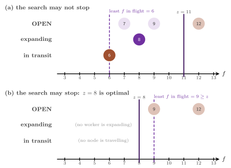
We draw the theorem in Figure 8.1: a search may stop when the least \(f\) in flight is at least the incumbent, and only then. In fact, the searches differ only in how they decide that this condition holds, which is easy when one lock or one master sees all the entries (SPA\(^*\) and the farm), needs a counter when the OPEN list is spread over many queues (MQA\(^*\)), and is the delicate part of a decentralized search, in which no worker sees the others at the same instant ([1], section 3.3.1). Once the search has stopped, the path is rebuilt from the recorded goal \(u\) through the parent pointers, after all the workers have returned. Its cost is at most the final \(g(u) \le z\) by the inequality of Lemma 2.10, which holds in the parallel searches at the end for the same reason as Lemma 2.6 in the proof above, and it is at least \(C^*\); hence it is exactly \(C^*\).
Proposition 8.7 (Finiteness). On a finite graph with nonnegative costs, a well-formed search creates finitely many entries. Hence, if each of its workers selects an entry, or waits, in a finite time, and a worker without an entry to select waits only for a step of another worker, the search stops.
Proof. An entry is created only when \(g(v)\) takes a new value, which is strictly smaller than the previous one and is the cost of a path from \(s_0\) to \(v\). The argument (i) of Theorem 2.11 shows that these values are finitely many for each of the finitely many states. Each selection removes an entry from the flight set; hence, after finitely many selections no entry is left and the stopping condition of the search (whose form is proved for each search below) is met. \(\square\)
On an infinite graph a parallel search needs at least what A\(^*\) needs, i.e., costs at least some \(\varepsilon > 0\), a finite branching and a reachable goal (argument (ii) of Theorem 2.11); with costs that only avoid nonpositive cycles it may run forever (the example after Theorem 2.11). We do not prove that these hypotheses suffice for every search of this chapter: the relaxed order of MQA\(^*\) (§8.6), for instance, gives no deterministic bound on how long an entry of small \(f\) may wait in its queue.
Remark 8.8 (Idle flags are not enough). A test of termination that only polls each worker, possibly twice in a row, whether it is idle is not sound when the entries travel in messages: worker 0 may send an entry of small \(f\) to worker 1 and become idle, while worker 1, idle, has not received it yet. Both answer "idle" in both rounds if the message is slow, the search stops, and the entry, which may be on the only optimal path, is lost. A sound test must also count the entries in transit, as condition (iii) of Definition 8.5 and Theorem 8.6 require. In this chapter, the centralized searches count them by construction (a counter under the lock of OPEN, an atomic counter, the tasks out at the master), as the proofs below show. The decentralized ones use the counting of Dijkstra and Scholten [35] in shared memory and the four counters of Mattern [11] over MPI, which Chapter 9 treats.
Finally, all the parallel searches of the library skip the move back
to the parent in an OperatorDomain (Domain.h:356), as the
sequential A\(^*\) does (§2.9 and
[4]): the inverse of a move costs as much
as the move, and therefore the parent is never reached more cheaply
through its child, and the lookup of about one successor in three of the
sliding-tile puzzles is saved. This keeps the searches well-formed, as
in the proof of Proposition 2.16. Indeed,
a worker reads the operator \(o\) of \(u\) together with \(g(u) = \gamma\)
(under the lock of \(u\), or on the master), and \(o\) is the move from the
node \(p\) that gave \(u\) that value; hence \(\gamma = g_0 + c(p, u)\), where
\(g_0\) is the value of \(g(p)\) at that time, and since \(g(p)\) never
increases, the skipped successor \(p\) has \(g(p) \le \gamma - c(p, u) \le
\gamma + c(u, p)\), as condition (b) requires.
8.4 Simple Parallel A*¶
The simplest parallel A\(^*\) lets the \(p\) workers share the two lists of the sequential search, i.e., each worker takes the best entry of the shared OPEN, expands its node and puts the successors back ([1], Algorithm 2, and section 2.2 of [3]). Thus, the order of the expansions is usually close to that of A\(^*\), but \(p\) nodes are expanded at once, and a node may be expanded before the node that gives it a cheaper path. There are no owners, hence no communication in the sense of (8.2), and the load is balanced by construction. Its price is the coordination, since each selection and each insertion goes through the lock of OPEN.
The algorithm¶
Algorithm 8.1 (SPA\(^*\)). Here, the lock \(L\) protects OPEN and the counter busy of the workers that hold an entry; the fields of the nodes that change are protected by the locks of CLOSED (§8.5), and \(z\) is atomic, i.e., it is read and written as one word, without a lock.
 1  procedure SPA*(s₀, p)
 2     CLOSED ← {s₀}, with g(s₀) ← 0;  OPEN ← {(f(s₀), g(s₀), s₀)}
 3     z ← ∞;  busy ← 0;  done ← false
 4     in parallel, on each worker i = 0, ..., p − 1 do
 5        while not done do
 6           lock L
 7           if OPEN has an entry of f < z then
 8              (f, g, u) ← the first entry of OPEN, removed
 9              busy ← busy + 1
10           else if busy = 0 then done ← true
11           unlock L
12           if no entry was removed then wait a little;  continue
13           F ← ∅;  lock u
14           if u is closed or g ≠ g(u) then u is not expanded  ▷ stale
15           else close u
16           unlock u
17           if u is expanded and u is a goal then
18              z ← min(z, g(u)), recording u if g(u) < z
19           else if u is expanded then
20              for each successor v of u with g(u) + c(u,v) + h(v) < z do
21                 g' ← g(u) + c(u, v);  lock v
22                 if v ∉ CLOSED or g' < g(v) then
23                    g(v) ← g';  parent(v) ← u;  v is not closed
24                    F ← F ∪ {(g' + h(v), g', v)}
25                 unlock v
26           lock L;  push the entries of F in OPEN;  busy ← busy − 1
27           unlock L
28     return the path to the goal of cost z, if z < ∞
This is the pseudocode of SPAStar.h:16. A worker takes the
lock of OPEN only twice per expansion, to select an entry (lines 6 to 11) and
to push all the successors of its node at once (lines 26 and 27). The
expansion itself, at lines 13 to 25, runs without it, and this is where
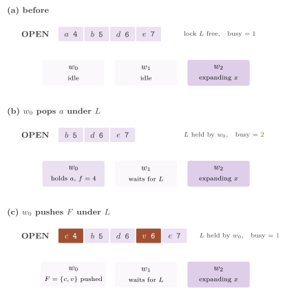
the parallelism is. Figure 8.2 draws one
selection and one insertion. At line 14, the test of staleness is the
lazy deletion of the sequential search, done under the lock of the node
since another worker may be lowering its \(g\). The goal test is at the
selection (line 17), and a goal does not end the search, which goes on
until line 10 finds no entry of \(f < z\) and no busy worker. The wait of
line 12 is an exponential backoff: the \(k\)-th consecutive wait spins for
\(2^k\) pauses of the processor, for \(k = 0, \ldots, 6\), and each further
wait yields the core to the system, so that a worker that finds OPEN
empty only for a moment does not sleep. When the node limit is set, a
worker that has stored that many nodes sets done and records that the
limit was hit, and the other workers leave the loop at line 5 after
their current step.
The code makes the expansion of lines 13 to 25 in two phases, which SPA\(^*\) and MQA\(^*\) share. In the first phase the worker generates the successors, prunes them by \(z\), computes their hashes and prefetches their places in CLOSED, i.e., it asks the processor to bring the lines of memory that their lookups will read into its cache without waiting for them (§3.8); in the second it updates them one by one. The cache misses of the lookups of all the successors therefore overlap, instead of following one another.
Algorithm 8.2 (The expansion of SPA\(^*\) and MQA\(^*\)). The entry \((\gamma + h(u), \gamma, u)\) has been selected; UPDATE is the operation of the shared CLOSED (Algorithm 8.3), and the procedure returns the set \(F\) of the entries to push.
 1  procedure EXPAND(u, γ)
 2     lock u
 3     if u is closed or g(u) ≠ γ then unlock u;  return ∅   ▷ stale
 4     close u;  read g(u) and the operator o of u;  unlock u
 5     if u is a goal then
 6        lock the goal record
 7        if g(u) < z then z ← g(u);  record u
 8        unlock the goal record;  return ∅
 9     S ← ∅                                  ▷ phase 1: no shared write
10     for each successor v of u not reached by the inverse of o do
11        if g(u) + c(u, v) + h(v) < z then
12           compute the hash of v;  prefetch its place in CLOSED
13           S ← S ∪ {(v, g(u) + c(u, v))}
14     F ← ∅                                  ▷ phase 2: the updates
15     for each (v, g') ∈ S do
16        if UPDATE(v, g', u) returns the node of v then
17           F ← F ∪ {(g' + h(v), g', v)}
18     return F
The incumbent is read at line 11 without any ordering of the memory (a
relaxed read): the value read is one that \(z\) had at some instant of
the expansion, and since \(z\) only decreases it is not smaller than the
current one, so that the pruning is the one that condition (b) of
§8.3 allows. The goal is recorded under a
separate mutex, taken only when a goal is selected. Furthermore, the
lock of OPEN starts a cache line, followed by OPEN and busy, which it
protects (SPAStar.h:216), the incumbent starts another one
(SPAStar.h:220), so that the reads of \(z\) at line 11 do not
share a line with the lock, and each worker with its counters starts a line of
its own (SPAStar.h:235); thus, the counters of two workers
never share a line.
Invariants and correctness¶
We now prove that SPA\(^*\) is correct. The proof rests on one invariant, which ties the counter busy to the entries that are not in OPEN.
Lemma 8.9 (The invariant of busy). Whenever \(L\) is free, and also while a worker holds \(L\) at line 7, every entry in flight is in OPEN or is held by one of the busy workers, i.e., by a worker between lines 9 and 26, and busy is the number of these workers.
Proof. Since SPA\(^*\) has no messages, an entry in flight is in OPEN or held (Definition 8.5). An entry leaves OPEN only at line 8, where the worker raises busy in the same critical section, and it is held (with the entries of \(F\) that it creates) until line 26, where the worker pushes \(F\) and lowers busy in the same critical section. Since both changes of busy are made under \(L\) together with the change of OPEN, the claim holds whenever \(L\) is released, and therefore also when it is taken again, until the worker that holds it changes OPEN or busy (which it does only after line 7). \(\square\)
Theorem 8.10 (Correctness and termination of SPA\(^*\)). If \(h\) is admissible and SPA\(^*\) ends without reaching the node limit, it returns an optimal path (or none, when no goal is reachable); on a finite graph with nonnegative costs it ends.
Proof. SPA\(^*\) is well-formed: (a) and (c) are lines 8, 24, 26 and 18, and (b) is lines 20 to 25, where the update of \(v\) is made under its lock, and where \(z\) is read without a lock, so that the pruning at line 20 uses a value that \(z\) had at some instant of the expansion (the successor skipped by the pruning of the parent of §8.3 is also allowed by (b)). When a worker sets done at line 10, it holds \(L\) and finds no entry of \(f < z\) in OPEN and busy \(= 0\). By Lemma 8.9 no entry in flight is held, and hence none has \(f < z\), and Theorem 8.6 gives \(z = C^*\). A worker that finds no entry to select at line 12 waits only for the busy workers, which end their expansion without waiting for anything but locks held for a bounded number of steps; hence Proposition 8.7 gives the termination. \(\square\)
Re-expansions¶
Unlike A\(^*\) (cf. Theorem 2.13), SPA\(^*\)
may expand a node more than once even with a consistent heuristic
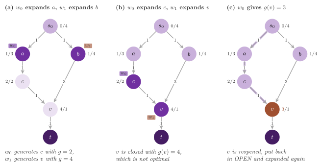
([1], section 3.2): in Figure
8.3, two workers expand \(a\) and \(b\) at
once, the second best entry \(b\) generates \(v\) through an expensive edge,
and \(v\) is selected and closed by \(w_1\) before \(w_0\), through \(c\), finds
the cheaper path to it. As one can check on the figure, lines 22 and 23
then reopen \(v\) (v is not closed), and it is expanded again; the
counter reexpanded counts these expansions, which belong to the search
overhead (8.1). With \(p = 1\), SPA\(^*\) is A\(^*\), and the re-expansions
are those of an inconsistent heuristic
(§2.7). The number of the re-expansions is
bounded as follows, for SPA\(^*\) and, with the same proof, for MQA\(^*\)
and the farm.
Lemma 8.11 (One expansion per value of \(g\)). In SPA\(^*\), MQA\(^*\) and the farm, between two expansions of a node \(u\) the value of \(g(u)\) strictly decreases. Hence, \(u\) is expanded at most as many times as the distinct values that \(g(u)\) takes, and the re-expansions are at most the decreases of \(g\) after a first expansion.
Proof. An expansion of \(u\) selects an entry \((u, \gamma)\) that is not stale, i.e., with \(u\) not closed and \(g(u) = \gamma\), and closes \(u\), in one critical section on the lock of \(u\) (lines 2 to 4 of Algorithm 8.2; in the farm, only the master does both). A later expansion needs an entry that is not stale, hence \(u\) not closed; but \(u\) is made not closed only by an update that sets \(g(u)\) to a strictly smaller value (line 23 of Algorithm 8.1, line 9 of Algorithm 8.3, the INSERT of the farm). \(\square\)
The lemma does not bound the decreases of \(g\) in terms of \(p\); they are bounded only by the number of the distinct costs of the paths to the node that are smaller than its first value of \(g\) (cf. Proposition 8.7), and we know no bound that depends on \(p\) alone. With \(p = 1\) and a consistent heuristic no decrease follows an expansion, and the lemma gives the single expansion of Theorem 2.13.
The cost of an expansion¶
We now count the synchronization of a step of SPA\(^*\), since it limits the search when the expansions are fast.
Proposition 8.12 (The cost of a step of SPA\(^*\)). A worker that selects an entry takes \(L\) twice (lines 6 and 26), the lock of \(u\) once, and, for each successor \(v\) that is not pruned, at most one lock of CLOSED (with the default data structures, only when \(v\) was already stored and \(g'\) improves on the \(g(v)\) read without the lock, cf. Lemma 8.13); under \(L\) it makes one removal and \(|F|\) insertions of the OPEN list. The nodes stored are one per state reached, and the entries pushed in OPEN, stale ones included, are one for each value taken by the \(g\) of a node, i.e., one for each state reached plus one for each later improvement of its \(g\).
Proof. The counts are read on Algorithms 8.1, 8.2 and 8.3; a worker that finds no entry to select takes \(L\) once and waits. Each state has one node by Lemma 8.13(i), and an entry is pushed only for the root and for each update that returns a node, i.e., for each new state or improvement of \(g\) (Lemma 8.13(iii)). \(\square\)
Hence, the lock of OPEN is contended by all the workers twice per expansion, and the survey reports that, when the expansions are as fast as on the sliding-tile puzzle, SPA\(^*\) is usually slower than the sequential A\(^*\), even with lock-free data structures ([1], section 3.2, after [3]). It may pay off when the expansions are slow, since the time under \(L\) is then a small part of an expansion. MQA\(^*\) (§8.6) removes this lock.
8.5 The shared closed list¶
SPA\(^*\) and MQA\(^*\) share one CLOSED list, the class
ConcurrentClosed< D , Lock > of ConcurrentClosed.h,
which maps each state to its canonical node and protects the fields of a node
that change during the search (\(g\), the parent, the operator and the flags
closed and expanded); \(h\) never changes and is read freely. Its operation
update( t , hash , g , h , parent , op , ... ) records the path to \(t\) of
cost \(g\): it returns the node of \(t\) when \(t\) is new or \(g\) is smaller than
its \(g\), which is then set with the parent and the operator and makes the node
not closed, and returns a null pointer otherwise, counting a duplicate. Its
implementation is chosen at build time with the set of data structures
(Structures.h, §3.12).
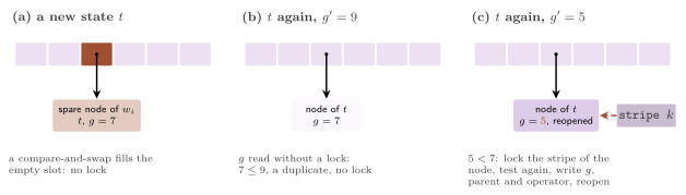
With the default data structures, CLOSED is a lock-free hash table of pointers to the nodes, compared by their states, one word of 8 bytes per node, which a lookup reads and an insertion fills by a compare-and-swap, i.e., an atomic instruction that writes a word only if it still holds the value read before. The fields that change are protected by 256 locks, each on a cache line of its own, the lock of a node being chosen by a multiplicative hash of its address. Each worker keeps a spare node, allocated from its private pool, which it fills with the state before the insertion and keeps for the next call when the state was already there. Figure 8.4 draws the three cases of the update, which the following procedure makes.
Algorithm 8.3 (The update of the shared CLOSED). The path to \(v\) of cost \(g'\) through \(u\) is recorded; the procedure returns the node of \(v\) when an entry must be pushed, and nil otherwise.
 1  procedure UPDATE(v, g', u)
 2     n ← the spare node of the worker, filled with v, g', h(v), u
 3     x ← the node of v in CLOSED, or n inserted by a compare-and-swap
 4     if x = n then the worker takes a new spare node;  return x
 5     if g' < g(x), read without the lock of x, then
 6        lock x
 7        if g' < g(x) then
 8           g(x) ← g';  parent(x) ← u;  the operator of x ← that of v
 9           x is not closed;  unlock x;  return x
10        unlock x
11     count a duplicate;  return nil
With the data structures of the standard library or of Boost, CLOSED is
split into 256 shards by the top byte of the hash of the state, each a
sequential table with a lock, which also protects the nodes of its
states (structures/std/ConcurrentClosed.h:134);
UPDATE then takes the lock of the shard of \(v\) and runs lines 3 to 11 under it,
with the test of line 5 dropped and the node allocated only when \(v\) is new;
the prefetch of Algorithm 8.2 then does nothing, since the table of a shard
may be reallocated under its lock.
We now show that the shared CLOSED loses no improvement of \(g\), although most of its operations take no lock. We assume of the lock-free table what its implementation guarantees and what we do not prove here, i.e., that the find-or-insert of line 3 is linearizable: of several calls on the same state, exactly one inserts its node, and the others return that node.
Lemma 8.13 (The lock-free update). With the lock-free table, (i) each state has at most one node; (ii) the \(g\) of a node never increases; (iii) if UPDATE returns nil, the \(g\) of the node was at most \(g'\) at some instant of the call, and if it returns the node, it has set \(g\) to \(g'\), which was smaller than \(g\) at that instant; and (iv) a call that finds \(g(x) \le g'\) at line 5 takes no lock and writes no field of a node. Hence no improvement of \(g\) is lost, and each improvement creates exactly one entry.
Proof. (i) Line 3 inserts a node only when the state is not in the table, by the assumption on the table. (ii) The only writes of \(g\) are the initialization of a new node at line 2, before it is published by line 3, and line 8, under the lock of the node, after the test of line 7 that the new value is smaller. (iii) The read of line 5 is an atomic read of the word of \(g\), and it returns a value that \(g\) had at some instant; since \(g\) never increases, the current value is not larger. If the value read is at most \(g'\), the current one is too, and the call is a duplicate. Otherwise the call takes the lock and tests again, and the test of line 7 and the write of line 8 are exact, since all the writes are made under that lock. (iv) Such a call executes lines 2, 3, 5 and 11, which write the spare node, private to the worker, its counter, and whatever the find-or-insert of line 3 writes in the table itself (with the default table, a counter of the calling thread on a cache line of its own, which a growth of the table reads), but no node. \(\square\)
The duplicates, which are often the most frequent case of a search with many transpositions, thus take no lock and write no node, except those that lose a race between lines 5 and 7, which take the lock of the node and then find \(g(x) \le g'\). A node is allocated once per state inserted; the nodes are never moved, and a pointer to a node stays valid until the end of the search (as the parent pointers and the entries of OPEN require).
8.6 MultiQueue A*¶
MQA\(^*\) keeps the shared CLOSED of SPA\(^*\) and replaces its OPEN, a priority queue under one lock, by a relaxed priority queue, the MultiQueue of Rihani, Sanders and Dementiev [37]: \(n = 2p\) sequential priority queues, each with a separate lock, a push into a queue drawn at random, and a pop from the better of two queues drawn at random (Figure 8.5). Two workers then contend only when they happen to draw the same queue (which is rather rare with \(2p\) queues), and even then the one that finds the lock taken draws again instead of waiting, while the order of the pops typically stays close to that of the keys.
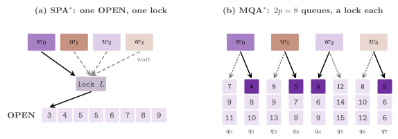
The MultiQueue¶
Each queue \(j\) keeps the key of its minimum in an atomic word
\(\mathit{top}_j\) (\(\infty\) when the queue is empty), which the other
workers read without its lock. A try-lock takes a lock only if it is
free, and returns at once otherwise. MQA\(^*\) uses the MultiQueue with a
stickiness of 1 (MQAStar.h:121), i.e., each operation
draws its queues anew, and with its successors pushed together, as follows.
Algorithm 8.4 (The MultiQueue of MQA\(^*\), with \(n\) queues).
 1  procedure PUSHALL(E)                  ▷ the entries E, into one queue
 2     loop
 3        j ← a queue drawn at random
 4        if a try-lock of j succeeds then break
 5     put the entries of E in the queue j;  top_j ← its least key
 6     unlock j
 7  function POP()
 8     loop
 9        j, j' ← two distinct queues drawn at random
10        if top_j' < top_j then j ← j'     ▷ read without the locks
11        if top_j = ∞ then return SCAN()
12        if a try-lock of j succeeds then break
13     if the queue j is empty then unlock j;  return SCAN()
14     e ← the least entry of j, removed;  top_j ← its least key, or ∞
15     unlock j;  return e
16  function SCAN()
17     for each queue j, from one drawn at random, do
18        lock j
19        if j is not empty then
20           e ← its least entry, removed;  update top_j;  unlock j
21           return e
22        unlock j
23     return nothing
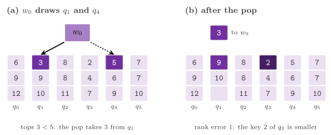
Each queue is exact, i.e., it removes its least entry: it is an 8-ary heap behind two buffers of 16 entries, a sorted one that holds its least entries and from which a pop takes, and an unsorted one that a push fills and that goes into the heap only when it is full or when the sorted one runs out. Hence, the pop returns an entry that is not always the least of all (Figure 8.6): its rank error is the number of the entries present with a smaller key. In the sequential model of the analysis (the entries spread at random over the \(n\) queues and removed by the better of two random queues), the expected rank error is linear in \(n\), and its maximum over a polynomial number of pops is \(O(n \log n)\) with high probability, while a pop from a single random queue would make it grow without bound; these are results of the literature recalled in [38], which we do not prove here, and they hold in that model, not for the interleavings of a real run. Since SPA\(^*\) expands \(p\) nodes at once anyway, a rank error of order \(n = 2p\) departs from the order of A\(^*\) by somewhat more than SPA\(^*\) already does, and arguably not by much. Also, POP returns nothing only after SCAN has found all the queues empty, each locked in turn; with pushes running at the same time this does not prove that the structure is empty (a push may fill a queue already scanned), and MQA\(^*\) therefore does not use it for its termination.
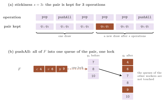
Two refinements of the MultiQueue save cache misses. A worker may keep
the two queues it drew for \(s\) operations, the stickiness, which keeps
their lines in its cache, and draw again after \(s\) operations or when a
lock is held (Figure 8.7). The rank
errors then grow (about linearly in \(s\), according to the measures
available, since there is no theory yet), and MQA\(^*\) uses \(s = 1\),
which keeps the model of the bounds above. Also, a worker that has
several entries to push at once, as the successors of a node, may push
them all into one queue under one lock (PUSHALL,
MQAStar.h:299). This takes one lock per expansion instead of
one per successor, and relaxes the order as a stickiness of \(|F|\) would, since
the successors of a node then sit in the same queue; MQA\(^*\) does so, and the
bounds of the model then no longer apply as stated.
The algorithm and its termination¶
Algorithm 8.5 (MQA\(^*\)). Here, OPEN is the MultiQueue of Algorithm 8.4 and the atomic counter \(m\) of the entries that are in OPEN or held by a worker replaces busy and the lock \(L\) of SPA\(^*\).
 1  procedure MQA*(s₀, p)
 2     CLOSED ← {s₀}, with g(s₀) ← 0;  OPEN ← {(f(s₀), g(s₀), s₀)}
 3     z ← ∞;  m ← 1;  done ← false
 4     in parallel, on each worker i = 0, ..., p − 1 do
 5        while not done do
 6           e ← a pop of OPEN, possibly nothing
 7           if no entry was popped then
 8              if m = 0 then done ← true
 9              else wait a little
10              continue
11           (f, g, u) ← e;  F ← ∅
12           if f < z then F ← EXPAND(u, g)          ▷ Algorithm 8.2
13           m ← m + |F| − 1;  push the entries of F in OPEN
14     return the path to the goal of cost z, if z < ∞
This is the pseudocode of MQAStar.h:19. Since the entries of
OPEN are not ordered across the queues, an entry popped with \(f \ge z\) does not
mean that OPEN has no better entry, and it is dropped (line 12) instead
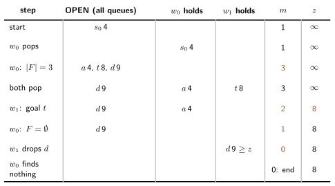
of ending the search. The end is decided by \(m\) only (Figure
8.8). The wait of line 9 is the backoff of
SPA\(^*\), and the node limit is handled as there.
We now show that \(m\) counts all the entries in flight, whatever the interleaving of the workers.
Lemma 8.14 (The invariant of \(m\)). At every instant, \(m = |\mathrm{OPEN}| + H + Q\), where \(|\mathrm{OPEN}|\) is the number of entries in the queues, \(H\) the number of the workers that hold a popped entry and have not yet executed the addition of line 13, and \(Q\) the number of entries that have been counted at line 13 and are still to be pushed. Hence \(m = 0\) if and only if OPEN is empty and no worker holds an entry.
Proof. At line 3, \(m = 1\) and OPEN holds the root. A pop (line 6) moves one entry from OPEN to a holding worker and leaves \(m\) unchanged. In turn, the atomic addition of line 13 ends the holding of one worker (\(H\) falls by 1) and counts the \(|F|\) entries to be pushed (\(Q\) rises by \(|F|\)), and it adds \(|F| - 1\) to \(m\) (when \(|F| = 1\) the code skips the addition, which would add 0, and the holding ends at the same point of line 13). Each push of line 13 moves an entry from \(Q\) to OPEN. The three terms are nonnegative, which gives the last claim. \(\square\)
The order of line 13 matters. Indeed, the entries of \(F\) are counted
before they are pushed, and therefore \(m\) never misses an entry. Had
they been counted after the pushes, another worker could pop one of
them, expand it and subtract its 1 before it was added, and read
\(m = 0\) while entries were still in flight. Also, the code makes one
atomic addition per expansion (MQAStar.h:293, an addition of
\(|F| - 1\) modulo \(2^{64}\), which is a subtraction of 1 when
\(F = \emptyset\)), and none when \(|F| = 1\), instead of one before and
one after the pushes, which halves the traffic on the cache line of \(m\).
All the workers share that line, on which \(m\) comes first
(MQAStar.h:249); we remark that the line is not padded after
\(m\), so that the first fields of CLOSED, which follow \(m\) in memory, may share
it.
Theorem 8.15 (Correctness and termination of MQA\(^*\)). If \(h\) is admissible and MQA\(^*\) ends without reaching the node limit, it returns an optimal path (or none, when no goal is reachable); on a finite graph with nonnegative costs it ends.
Proof. MQA\(^*\) is well-formed for the reasons given for SPA\(^*\) in Theorem 8.10, the expansion being the same (Algorithm 8.2), and an entry dropped at line 12 has \(f \ge z\), to which condition (b) does not apply. A worker sets done only when it reads \(m = 0\), and then, by Lemma 8.14, no entry is in OPEN and none is held, i.e., none is in flight, and Theorem 8.6 gives \(z = C^*\). A worker whose pop fails while \(m > 0\) waits for the workers that hold entries or are about to push them, and these end their step without waiting for anything but locks of single queues; Proposition 8.7 gives the termination. \(\square\)
The order of the pops changes only how many nodes are expanded before \(z\) is optimal and how many are reopened, never the cost of the path.
Proposition 8.16 (The cost of a step of MQA\(^*\)). A step of a worker that pops an entry takes one lock of a queue for the pop and one for PUSHALL (none when \(F = \emptyset\)), the locks of Algorithm 8.2, and at most one atomic addition on \(m\); unlike the lock \(L\) of SPA\(^*\), none of these locks is taken by every step of every worker. Each operation on a queue \(j\) costs that of the 8-ary heap of \(j\), i.e., \(O(\log |q_j|)\) comparisons in the worst case, \(|q_j|\) being the number of entries of \(j\).
Proof. The counts are read on Algorithms 8.4 and 8.5; PUSHALL takes one lock for all the entries of \(F\), and the addition of line 13 is skipped when \(|F| = 1\). The locks of a failed try-lock are not taken. The cost of a heap is that of §3.2, the buffers only lowering it on average. \(\square\)
The proposition does not bound the number of the draws of a pop, which grows with the contention for the queues; we have no bound on it in a real run, beyond the remark that with \(2p\) queues and at most \(p - 1\) other locks held at any instant a draw finds a free queue rather often.
The key of OPEN¶
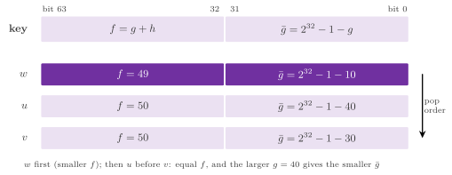
With integer costs the key of an entry of MQA\(^*\) (and of PA\(^*\)SE) is the packed word of §3.4,
i.e., \(f\) in the high half and the complement of \(g\) in the low half (Figure 8.9), so that the comparison of two keys is one comparison of integers and gives the order of Lemma 3.6: by increasing \(f\) and, for equal \(f\), by decreasing \(g\), provided that \(g, h \ge 0\) and \(g + h < 2^{32}\), which the integer costs of the domains of the library satisfy by a wide margin. With real costs the key is \(f = g + h\) alone, and the ties are broken by the queues. Line 12 of Algorithm 8.5 reads \(f\) from the key by the shift above.
The preference of the deeper node within a layer of equal \(f\) matters for a relaxed queue rather more than for an exact one, as we now explain. The last layer \(f = C^*\) often holds a large part of the nodes (on the sliding-tile puzzles, for instance), and a search that prefers the deeper nodes typically reaches a goal after a part of that layer (§2.8). With \(f\) only, instead, the pops of the layer come in an arbitrary order, and typically much more of it is expanded before a goal is found. Since a MultiQueue scatters the entries of one layer over \(2p\) queues, only the key can carry the preference for depth into each of them.
As for the expansion and CLOSED, the engineering is that of SPA\(^*\)
(prefetches, cache lines, lock-free duplicates). Finally, the test
mqa-thread runs MQA\(^*\) with 1, 2, 3 and 8 workers on two instances of
Korf of the 15-puzzle and on the map of Romania, and with 8 and with 0
workers (which normalize() turns into 1) on the corner cases of
check_astar_edges (e.g., an initial state that is a goal, one move and
a node limit); mqa-openmp does the same on OpenMP.
8.7 The master-worker farm¶
The farm with feedback is a master-worker form of the centralized
approach of section 3.2 of [1], written with
the farm of the executor of the library (a farm of FastFlow
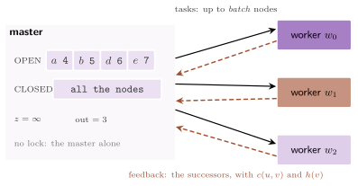
[12] on that runtime). A master owns OPEN,
CLOSED, all the nodes and the incumbent, and therefore needs no lock. It
sends the best nodes of OPEN, in tasks of up to batch nodes, to the
workers that are free (the farm schedules them on demand). A worker
generates the successors of the nodes of its task, with their costs and
their heuristic values, and sends them back on the feedback channel
(Figure 8.10). The master then checks
them against CLOSED and puts the new and the improved ones in OPEN. In
other words, the scheme is that of SPA\(^*\) with the master in the place
of the locks.
Algorithm 8.6 (The farm). INSERT is the insertion of the sequential A\(^*\) on the lists of the master (a new state goes in OPEN; a state reached with a smaller \(g\) is updated, reopened and put in OPEN again; otherwise it is a duplicate), and the stale entries of OPEN are dropped when they reach its top, as in A\(^*\).
 1  procedure MASTER(s₀, p)
 2     z ← ∞;  out ← 0;  INSERT(s₀, 0, nil)
 3     loop
 4        DISPATCH()
 5        if out = 0 and OPEN has no node of f < z then return
 6        receive a task T back from a worker;  out ← out − 1
 7        for each successor v of a node u of T, with c(u, v) and h(v) do
 8           if g(u) + c(u, v) + h(v) < z then INSERT(v, g(u) + c(u, v), u)
 9  procedure DISPATCH()
10     while out < p and OPEN has a node of f < z do
11        T ← ∅
12        while |T| < batch and OPEN has a node of f < z do
13           u ← the first node of OPEN, removed;  close u
14           if u is a goal then z ← min(z, g(u)), recording u if g(u) < z
15           else T ← T ∪ {u}
16        if T = ∅ then return
17        send T to a free worker;  out ← out + 1
18  procedure WORKER(T)                       ▷ on each of the p workers
19     for each u ∈ T, add to T the successors v of u, with c(u, v), h(v)
20     send T back to the master
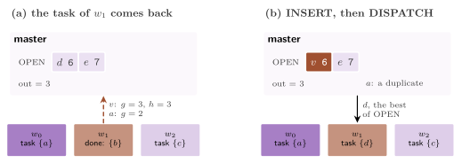
This is the pseudocode of FarmAStar.h:17; the goal test is
at the selection (line 14), which is the expansion point of the master, and
Figure 8.11 draws one return of a task.
A task carries, for each of its nodes, the pointer to the node and a
copy of its operator, and the worker reads of a node only its state and
its \(h\), which never change; hence the master may update the other
fields of a node that is out (its \(g\), its parent, its operator) without
a race. Lines 6 to 8 are made in two phases, as the expansion of
SPA\(^*\) is.
Algorithm 8.7 (The return of a task, on the master).
 1  function BACK(T)
 2     out ← out − 1
 3     for each successor v in T do              ▷ phase 1
 4        compute the hash of v;  prefetch its place in CLOSED
 5     for each successor v of a node u of T, with c(u, v) and h(v) do
 6        if g(u) + c(u, v) + h(v) < z then INSERT(v, g(u) + c(u, v), u)
 7     if the master stores at least node_limit nodes then
 8        the limit is hit, and DISPATCH sends nothing more
 9     put T in the list of the free tasks;  DISPATCH()
10     return out > 0 or (the limit is not hit and OPEN has a node of f < z)
The farm of the executor calls BACK on each task that comes back, and it ends when BACK returns false, i.e., when the test of line 5 of Algorithm 8.6 holds (or the limit is hit and no task is out). The tasks are reused through the list of free tasks, and the farm allocates no memory for them in the steady state.
As for SPA\(^*\), the correctness of the farm rests on an invariant, here on the counter out, from which Theorem 8.6 applies.
Lemma 8.17 (The invariant of out). Whenever the master is between two of its steps (at line 5 of Algorithm 8.6, or at the end of BACK), every entry in flight is in OPEN or belongs to one of the tasks that are out, as one of their nodes or as a successor of one, and out is the number of these tasks.
Proof. Only the master changes OPEN, \(z\) and out, and it handles one returned task at a time. An entry leaves OPEN only at line 13, and it is either a goal, processed at once (line 14), or put in a task \(T\), which leaves at line 17 with out raised by 1. The task holds its nodes and then their successors until it comes back, when line 6 lowers out by 1 and lines 7 and 8 insert the successors that are not pruned, before the master's next step. \(\square\)
Theorem 8.18 (Correctness and termination of the farm). If \(h\) is admissible and the farm ends without reaching the node limit, it returns an optimal path (or none, when no goal is reachable); on a finite graph with nonnegative costs it ends.
Proof. The search is well-formed: a node selected at line 13 is either a goal (line 14) or carried in a task, whose successors are inserted at line 8, before the next test of line 5. Note that \(g(u)\) at line 8 is the current \(g\) of the parent, which may be smaller than when the task left, if \(u\) was improved meanwhile. It is still the cost of a path to \(u\), and \(g(u) + c(u, v)\) is therefore the cost of a path to \(v\), and \(u\), reopened, is selected again. By Lemma 8.17, out \(= 0\) and no node of \(f < z\) in OPEN mean that no entry with \(f < z\) is in flight, and Theorem 8.6 gives \(z = C^*\). A worker never waits for anything but a task, and the master waits at line 6 only when out \(> 0\); Proposition 8.7 gives the termination. \(\square\)
Proposition 8.19 (The work of the master). At any instant at most \(p\) tasks, and hence at most \(p \cdot \mathrm{batch}\) nodes, are out at the workers. For each task of \(b\) nodes whose successors are \(S\), the master makes \(b\) removals of non-stale entries from OPEN (besides the stale entries it drops on the way), \(|S|\) computations of a hash, at most \(|S|\) lookups in CLOSED and at most \(|S|\) insertions in OPEN, while the workers generate the \(|S|\) successors in parallel.
Proof. Line 10 dispatches only while out \(< p\), and a task has at most batch nodes (line 12). The counts follow from Algorithms 8.6 and 8.7: each successor is hashed in the first phase of BACK, and it is passed to INSERT, which makes one lookup and at most one insertion, unless it is pruned. \(\square\)
Since the master does all the bookkeeping (the lookups in CLOSED, the
updates of OPEN and the selections), it is typically a bottleneck unless
the generation of the successors, the only part done by the workers in
parallel, costs much more than the bookkeeping of the same successors.
Also, the batch trades the number of the tasks against the order of the
expansions, since the nodes of a task are the batch best of OPEN at the
time of the dispatch, not at the time of their expansion. The farm runs
threads + 1 threads, and with PBEFS_PIN the master takes the first
core of the affinity mask and the worker \(i\) the core \(i + 1\)
(FarmAStar.h:186). Finally, the test farm-thread (and
farm-openmp, farm-fastflow) runs the farm with 1, 2, 3 and 8 workers and
tasks of 1 and of 4 nodes, on the 15-puzzle, on a random grid and on the map of
Romania, proves a grid split by a wall unsolvable, checks the node limit
and, with 8 workers and with the number of workers and the batch at 0,
the corner cases of check_astar_edges.
8.8 Parallel A* for slow expansions¶
The searches above expand in parallel nodes whose \(g\) may not be optimal yet, and pay for it with re-expansions. PA\(^*\)SE of Phillips, Likhachev and Koenig [6] expands in parallel only states whose \(g\) is already optimal (or within a factor of it), proved so by a pairwise heuristic, at the price of a test before each expansion; hence, no state is expanded twice. With a weight \(w > 1\) on the heuristic it is the wPA\(^*\)SE of section 4 of [6].
Independence and safety¶
Let \(h(t, s)\) be the pairwise heuristic of the domain, an estimate of
the cost \(d(t, s)\) of a path from \(t\) to \(s\), and let \(h(s)\) be the
heuristic of the search, an estimate of the cost \(h^*(s)\) from \(s\) to
the nearest goal. PA\(^*\)SE needs the following properties, which we call
(H): (H1) \(h(t, s) \le d(t, s)\) for all \(t\) and \(s\) (the pairwise
heuristic is admissible), (H2) \(h\) is admissible, and (H3)
\(h(t) \le h(t, s) + h(s)\) for all \(t\) and \(s\) (the forward-backward
consistency of [6], a triangle inequality
that the paper states for \(h(\cdot, \cdot)\), in the form that the proofs
below use; it holds when \(h(t)\) is the pairwise heuristic to the nearest
goal). The library leaves them to the Domain
(Domain.h:295); the pairwise heuristics of the library are
the distance between two cells of a grid, the sum of the displacements of the
tiles of a sliding-tile puzzle and the number of the cells that are dirty in
\(t\) and clean in \(s\) of the vacuum world, each with the matching heuristic
\(h\) (the distance to the goal cell, the Manhattan distance and the
number of the dirty cells), and each satisfies (H) since it is a
distance, or a count of the moves that remain, for which the triangle
inequality holds. OPEN is ordered by \(f' = g + w h\), with \(w \ge 1\) the
weight of the options (1 for PA\(^*\)SE), and the inflation \(\varepsilon_p\)
of the test below is at least \(w\) (the constructor raises it to \(w\) when
it is smaller, PASE.h:222-239).
Definition 8.20 (Independence and safety). For \(\varepsilon_p \ge 1\), a state \(s\) is independent of a state \(t\) if
A state \(s\) of OPEN is safe if it is independent of each state \(t\) being expanded (the set BE, with its \(g\) at the expansion) and of OPEN with \(f'(t) < f'(s)\).
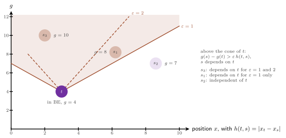
Intuitively, a path through \(t\) reaches \(s\) with a cost at least \(g(t) + d(t, s) \ge g(t) + h(t, s)\); hence, if \(s\) is independent of \(t\), such a path cannot lower \(g(s)\) below \(g(s) / \varepsilon_p\) (for \(g(t)\) optimal). The states \(t\) with \(f'(t) \ge f'(s)\) need no check, since \(s\) is independent of them: by (H3), \(f'(s) \le f'(t)\) and \(w \le \varepsilon_p\) give
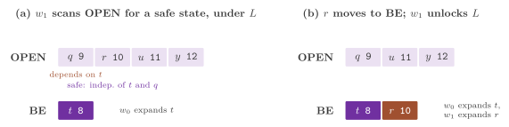
which is Theorem 2 of [6] for OPEN, and the same argument for BE, whose states keep the \(g\) of their expansion (it is the observation of the section "Algorithm" of GePA\(^*\)SE [122]). Figure 8.12 draws (8.4) on a line of states: the states that depend on \(t\) are those above a cone with its apex in \(t\) and slopes \(\pm \varepsilon_p\), and a larger \(\varepsilon_p\) makes the cone steeper and more states independent.
The algorithm¶
Algorithm 8.8 (PA\(^*\)SE). One lock \(L\) protects OPEN, BE and CLOSED; OPEN is an ordered set by increasing \(f'\) and, for equal \(f'\), by decreasing \(g\), CLOSED holds all the states generated, each with the flag closed, and \(K\) is the number of the states of OPEN examined (all, if 0).
 1  procedure PA*SE(s₀, p)
 2     CLOSED ← {s₀}, with g(s₀) ← 0;  OPEN ← {s₀};  BE ← ∅
 3     in parallel, on each worker do
 4        lock L
 5        while not done do
 6           s ← the first state of OPEN, among its first K, that is SAFE
                and, if a goal, ENDS
 7           if there is none then
 8              if OPEN = ∅ and BE = ∅ then done ← true;  break
 9              wait on L until OPEN or BE change;  continue
10           remove s from OPEN
11           if s is a goal then record s;  done ← true;  break
12           add s to BE;  close s;  unlock L
13           S ← the successors of s, with their costs   ▷ the slow part
14           lock L
15           for each (v, c(s, v)) ∈ S do
16              g' ← g(s) + c(s, v)
17              if v ∉ CLOSED then
18                 add v to CLOSED and OPEN, with g(v) ← g', parent(v) ← s
19              else if v is not closed and g' < g(v) then
20                 g(v) ← g';  parent(v) ← s;  reorder v in OPEN
21           remove s from BE;  wake the waiting workers
22        unlock L
23  procedure SAFE(s)
24     for each t ∈ BE with f'(t) < f'(s) do
25        if g(s) − g(t) > ε_p h(t, s) then return false
26     for each t ∈ OPEN with f'(t) < f'(s) do
27        if g(s) − g(t) > ε_p h(t, s) then return false
28     return true
29  procedure ENDS(s)
30     return no state t of OPEN ∪ BE has g(t) + ε_p h(t) < g(s)
This is the pseudocode of PASE.h:18, i.e., Algorithm 1 of
[6] with the scan of line 6 bounded, the test
of BE restricted to the states of smaller key by (8.5), and the test ENDS
for the goals. The wait of line 9 is on a condition variable, which
releases \(L\) and suspends the worker in one atomic step until another
worker wakes it (line 21), and then takes \(L\) again. Figure
8.13 draws one selection, in which the
first state of OPEN depends on the state being expanded and is skipped,
and the second is safe and moves to BE. Note that, by line 19, a closed
state is never improved and never reopened, which is sound only because
of Lemma 8.21 below. The code makes the selection as follows, with the
options candidates (\(K\), 64 by default) and prune (true by default)
and with \(z\) the least \(g\) of a goal in OPEN (\(\infty\) if none), which the
insertions of line 18 and 20 keep (PASE.h:377-441
and 453-476).
Algorithm 8.9 (The selection of PA\(^*\)SE, under \(L\)).
 1  function SELECT()
 2     for each x of OPEN, in order, until K pass line 3 (all if K = 0), do
 3        if PRUNED(x) then continue
 4        if SAFE(x) and (x is not a goal or ENDS(x)) then return x
 5     return nil
 6  function SAFE(s)
 7     for each t of BE, and then of OPEN, in the order of the set, do
 8        if f'(t) ≥ f'(s) then go on with the next set
 9        if not (t is in OPEN and PRUNED(t)) and not INDEPENDENT(s, t)
             then return false
10     return true
11  function ENDS(s)
12     for each t of OPEN, and then of BE, in order, with f'(t) < g(s) do
13        if g(t) + ε_p h(t) < g(s) then return false
14     return true
15  function INDEPENDENT(s, t)
16     δ ← 0 with integer costs, 1e−9 · max(1, |g(s)|) with real costs
17     return g(s) − g(t) ≤ ε_p h(t, s) + δ
Here PRUNED(\(x\)) holds when prune is set, \(x\) is not a goal and \(g(x) +
\varepsilon_p h(x) \ge z\); SAFE does not check the pruned states of OPEN,
of which a selected state is independent anyway (the proof of Lemma 8.21).
The scans of lines 7 and 12 stop at the first state whose key is not
smaller, since OPEN and BE are sorted by \(f'\) first; with integer costs
the key is the packed word of §8.6 of
\(f'\) and \(g\), followed by the address of the node, and with real costs
the pair \((f', -g)\) followed by the address, which makes the keys
distinct. Thus, the states of equal \(f'\) are not checked, as (8.5)
allows, and a layer of equal \(f'\) costs a scan of BE per state instead of
a scan of the layer. ENDS needs only the states of key below \(g(s)\),
since a state \(t\) with \(f'(t) \ge g(s)\) has \(g(t) + \varepsilon_p h(t)
\ge f'(t) \ge g(s)\) (\(w \le \varepsilon_p\)). The tolerance \(\delta\) of line
16, the cost_slack() of Node.h with the relative tolerance
real_cost_tolerance, keeps the rounding of real costs from making the
goal depend on the states of equal \(f'\); with real costs, Lemma 8.21 and
Theorem 8.22 are therefore proved only for the exact test, and we do not
quantify how the tolerance, and the rounding of \(g\) along a path, weaken
their bounds. With integer costs the weight is the fraction \(w = a / b\),
with \(b = 1\) if \(w\) is an integer and \(b = 256\) otherwise (\(a\) rounded up,
so that the weight is not smaller than the one given), and the key is
\(b g + a h\), exact, packed with \(g\) in one word, which needs \(b g + a h <
2^{32}\); the Solution of a goal of cost \(c\) carries the lower bound
\(\lceil c / \varepsilon_p \rceil\) (\(c / \varepsilon_p\) with real costs) on
\(C^*\) (PASE.h:222-239 and 287-295).
Correctness¶
We first show that a state found safe has a nearly optimal \(g\); this is the invariant that allows line 19 to leave the closed states alone. Call a state done if it is closed and outside BE, i.e., its expansion is complete.
Lemma 8.21 (Safe states are nearly optimal). Under (H), with \(w \le \varepsilon_p\) and integer costs or the exact test, each state \(s\) that PA\(^*\)SE selects has \(g(s) \le \varepsilon_p \, g^*(s)\); with \(\varepsilon_p = 1\), each state is expanded with its optimal \(g\), and hence at most once.
Proof. By induction on the selections (cf. the proof of Theorem 8.6, of which this is the analogue for BE). Suppose that the states selected before have been selected with \(g \le \varepsilon_p g^*\), and that \(s\) is found safe with \(g(s) > \varepsilon_p g^*(s)\). Let \(P\) be an optimal path from \(s_0\) to \(s\), and let \(t\) be the first state of \(P\) that is not done; it exists, since \(s\) is in OPEN. We first show that \(t\) is in OPEN or in BE, with \(g(t) \le \varepsilon_p g^*(t)\). If \(t\) is closed, it is in BE, since it is not done, and it was selected before \(s\), so that the induction hypothesis gives the bound. Otherwise, if \(t = s_0\), then \(t\) is in OPEN with \(g(t) = 0\). Otherwise the predecessor \(t'\) of \(t\) on \(P\) is done, and it was selected with \(g(t') \le \varepsilon_p g^*(t')\); its expansion generated \(t\) (the successor that the pruning of the parent of §8.3 skips is the node whose expansion gave \(t'\) its \(g\), which is closed, while \(t\) is not), found \(t\) not closed (a state closed then would be closed now), and lines 17 to 20 left \(t\) in OPEN with \(g(t) \le g(t') + c(t', t) \le \varepsilon_p (g^*(t') + c(t', t)) = \varepsilon_p g^*(t)\), using \(\varepsilon_p \ge 1\) and \(c \ge 0\); \(g(t)\) has not increased since. Furthermore, \(t \ne s\), since, if \(t = s\), the bound just proved contradicts the assumption on \(s\). Since \(t\) precedes \(s\) on an optimal path, \(g^*(s) = g^*(t) + d(t, s)\), and
by (H1), so that \(s\) depends on \(t\). If \(t\) is a pruned state of OPEN, then \(g(t) + \varepsilon_p h(t) \ge z\), while \(g(s) + \varepsilon_p h(s) < z\) if \(s\) is not a goal (line 3 did not skip it), and \(g(s) \le g(t) + \varepsilon_p h(t)\) if \(s\) is a goal (ENDS(\(s\)) holds); in both cases \(g(s) - g(t) \le \varepsilon_p (h(t) - h(s)) \le \varepsilon_p h(t, s)\) by (H3), with \(h(s) = 0\) for a goal, and \(s\) is independent of \(t\). Otherwise, if \(f'(t) < f'(s)\), the state \(t\), in BE or in OPEN, is checked by SAFE (lines 24 to 27), and \(s\) is not safe; if \(f'(t) \ge f'(s)\), then \(s\) is independent of \(t\) by (8.5). All the cases contradict the dependence just shown. With \(\varepsilon_p = 1\) the bound is \(g(s) = g^*(s)\), and a state, once closed, is never put back in OPEN (line 19). \(\square\)
For the goal returned at line 11, safety is not enough when there are several goal states: Lemma 8.21 bounds \(g(s)\) by \(\varepsilon_p g^*(s)\), the cost of a cheapest path to that goal, which may exceed \(\varepsilon_p C^*\), and a safe goal may be returned while a goal of smaller \(f\) is still waiting. Algorithm 1 of [6] and its theorems are stated for one goal state; the test ENDS of line 6 extends the bound to a goal region.
Theorem 8.22 (Bounded suboptimality of
PA\(^*\)SE). Under (H), with \(w \le \varepsilon_p\) and integer costs or the
exact test, if PA\(^*\)SE returns a goal \(s\), then \(g(s) \le \varepsilon_p
C^*\); with \(\varepsilon_p = 1\) the path returned is optimal. The pruning of
the option prune does not change the bound.
Proof. Let \(P\) be an optimal path to a goal \(s'\), with \(g^*(s') = C^*\), and let \(t\) be the first state of \(P\) that is not done when \(s\) is selected. As in the proof of Lemma 8.21, \(t\) is in OPEN or in BE with \(g(t) \le \varepsilon_p g^*(t)\) (with the \(g\) of its expansion if in BE), and by (H2) and \(h^*(t) = C^* - g^*(t)\) (since \(t\) is on an optimal path)
ENDS(\(s\)) holds when \(s\) is selected, i.e., no state of OPEN or BE has \(g + \varepsilon_p h < g(s)\); hence \(g(s) \le g(t) + \varepsilon_p h(t) \le \varepsilon_p C^*\) (if \(t = s\), the same inequality holds with \(h(s) = 0\)). The pruning of line 3 of Algorithm 8.9 skips only states \(x\) with \(g(x) + \varepsilon_p h(x) \ge z\), the \(g\) of a goal in OPEN: it never skips a goal, and if it skips the state \(t\) above, then \(z \le \varepsilon_p C^*\), and the goal of cost \(z\) is already within the bound (the selections do not depend on the pruning in the argument above, which uses only ENDS). Finally, the path rebuilt through the parents has cost at most \(g(s)\), as in Lemma 2.10, since all the writes of \(g\) and of the parents are made under \(L\). \(\square\)
These are Theorems 1 and 3 of [6], stated
there for one goal state; the proofs above make explicit where the
forward-backward consistency (H3) enters, i.e., only in (8.5), which
restricts the checks to the states of smaller key. Exercise 8.6 asks for a
graph with two goal states on which the test of safety alone returns a goal
beyond the bound; the documentation of the library
(docs/theory/parallel-astar.md) reports that, before
ENDS, the test of safety alone returned paths up to 4% longer than the optimum
on 8 of the 50 navigation instances of the map den520d with 5 workers (a count
that we have not rerun).
Finally, we show when PA\(^*\)SE neither waits forever nor runs forever.
Proposition 8.23 (Progress and termination of PA\(^*\)SE). Let OPEN be not empty and BE empty, and let \(x\) be the first state of OPEN that line 3 of Algorithm 8.9 does not skip. Then SELECT returns \(x\). Hence no worker waits forever while another could proceed, and on a finite graph PA\(^*\)SE ends, with a goal or with OPEN and BE empty, in which case no goal is reachable.
Proof. The state \(x\) exists, since a goal in OPEN is never skipped and, without a goal in OPEN, \(z = \infty\) skips nothing. Each state \(t\) of OPEN before \(x\) is skipped, i.e., \(g(t) + \varepsilon_p h(t) \ge z > g(x) + \varepsilon_p h(x)\) (or \(x\) is a goal, with \(g(x) = z\), see below), and SAFE does not check it (line 9), while BE is empty; hence \(x\) is safe, and it is among the first \(K\) states examined, since the skipped ones are not counted (line 2). If \(x\) is a goal, then \(g(x) = z\), since a goal of \(g = z\) has \(f' = g\) not larger than that of \(x\) and comes first; the states before it are skipped, so that \(g(t) + \varepsilon_p h(t) \ge z = g(x)\), and the states after it have \(f' \ge g(x)\); hence ENDS(\(x\)) holds. A worker waits at line 9 only when no state is selected, i.e., when BE is not empty, while another worker expands outside \(L\). That worker then takes \(L\), changes BE at line 21 and wakes all the waiting workers, and no wake-up is lost, since the wait releases \(L\) atomically and all the changes are made under \(L\). By line 19 a closed state never re-enters OPEN, so that each state is closed at most once, and on a finite graph the selections are therefore finitely many. When OPEN and BE are both empty, all the states reachable from \(s_0\) have been closed, since the successors of a closed state were all added at line 18, and no goal was selected, so that none is reachable. \(\square\)
We remark that the proposition relies on two choices of the code
(PASE.h:399-416 and 456-461): the states skipped at line
3 do not count among the \(K\) states examined, and SAFE does not check the
pruned states of OPEN. Were they counted, with prune and \(K > 0\) the first
\(K\) states of OPEN could all be skipped while BE is empty, which is possible
when \(\varepsilon_p > w\) or with many states of \(f' = z\) and \(h = 0\), and no
state would be selected; were they checked, the first state not skipped would
be independent of them under (H3), as in the proof of Lemma 8.21, but with a
pairwise heuristic that violates (H3) it could depend on one of them, and again
no state would be selected. In either case each worker would wait at line 9 for
a change that no worker makes. Since the goal of cost \(z\) is in OPEN until it
is selected, and it is never skipped, the scan always reaches a state that is
not skipped.
The next proposition states in one place what the two choices preserve; the comment of SAFE in the code refers to it.
Proposition 8.24 (The pruning in the selection).
Under (H), with \(w \le \varepsilon_p\), \(\varepsilon_p \ge 1\), integer costs or
the exact test, and prune set, let SAFE not check the pruned states of OPEN
and let the \(K\) candidates of SELECT be counted among the states not pruned,
as in Algorithm 8.9. Then (i) the workers never all wait with OPEN not empty
and BE empty, and (ii) a goal \(s\) returned by PA\(^*\)SE has \(g(s) \le
\varepsilon_p C^*\).
Proof. (i) With BE empty, the first state \(x\) of OPEN not pruned is among the candidates and is safe, and if it is a goal it has \(g(x) = z\) and ENDS(\(x\)) holds (Proposition 8.23); hence SELECT returns a state. (ii) Since \(z\) is the least \(g\) of a goal in OPEN, it never increases, and the goal of cost \(z\) stays in OPEN until a goal is selected, since line 3 never skips a goal. Let \(P\) be an optimal path from \(s_0\) to a goal, so that \(g^*(v) + h^*(v) = C^*\) for each state \(v\) of \(P\). We show, by induction on the selections, that each state \(v\) of \(P\) is selected with \(g(v) \le \varepsilon_p g^*(v)\) unless \(z \le \varepsilon_p C^*\) already holds. Let \(v\) be selected with \(g(v) > \varepsilon_p g^*(v)\), and let \(q\) be the first state not done of an optimal path from \(s_0\) to \(v\), followed by the part of \(P\) after \(v\), which is an optimal path to the goal; as in the proof of Lemma 8.21, \(q \ne v\), \(q\) is in OPEN or BE with \(g(q) \le \varepsilon_p g^*(q)\) (the states before it are done, and selected with that bound by the induction, unless \(z \le \varepsilon_p C^*\) already, which is the claim), and \(v\) depends on \(q\). If \(q\) is checked by SAFE, or if \(f'(q) \ge f'(v)\), the dependence is contradicted as in that proof; otherwise \(q\) is a pruned state of OPEN, i.e., \(g(q) + \varepsilon_p h(q) \ge z\), and by (H2)
When the goal \(s\) is selected, ENDS(\(s\)) holds; if \(z \le \varepsilon_p C^*\), then \(g(s) \le z\), since the goal of cost \(z\) is in OPEN or is \(s\), and \(g(s) \le \varepsilon_p C^*\); otherwise the first state not done of \(P\) has \(g \le \varepsilon_p g^*\), and the argument of Theorem 8.22 gives the bound. \(\square\)
We remark that the hypotheses of the proposition are those of Theorem 8.22,
and that (ii) uses (H3) only through (8.5) and the selection of each state at
most once (line 19); the same argument holds for ePA\(^*\)SE, whose SAFE skips
the pruned states of OPEN and whose scan does not count them
(EPASE.h:584-587), with \(\bar g\) for the states of BE.
Proposition 8.25 (The cost of a selection). Under \(L\), a call of SELECT evaluates the pairwise heuristic at most \(K\,(|\mathrm{BE}_{<}| + |\mathrm{OPEN}_{<}|)\) times (\(|\mathrm{OPEN}|\) in place of \(K\) if \(K = 0\)), where \(\mathrm{BE}_{<}\) and \(\mathrm{OPEN}_{<}\) are the states of BE and of OPEN with \(f'\) smaller than that of the last candidate scanned, and \(|\mathrm{BE}| < p\); ENDS reads at most \(|\mathrm{OPEN}| + |\mathrm{BE}|\) states per goal examined. Each insertion in OPEN, removal and reordering costs \(O(\log |\mathrm{OPEN}|)\) in the ordered set, and the successors of an expansion cost one lookup in CLOSED each, under \(L\).
Proof. SELECT tries at most \(K\) candidates, and SAFE makes one test per state of BE and per state of OPEN before the candidate with a smaller \(f'\); BE holds the states being expanded, at most one per other worker. OPEN and BE are B-trees, whose operations are logarithmic, and lines 15 to 20 make one lookup per successor. \(\square\)
The engineering¶
We now turn to the implementation, which we have kept close to the
pseudocode. OPEN and BE are ordered sets (B-trees of the default data
structures, PASE.h:357-358). The scan of line 6 is
bounded by \(K\) states, which bounds the time under \(L\) (a state further
down would have to be checked against a longer and longer prefix of OPEN),
and by Proposition 8.23 the bound costs no progress under its condition.
Also, the hashes of the successors are computed outside \(L\), and under
\(L\) their places in CLOSED are prefetched before any lookup, and the
lock is therefore held for about one cache miss instead of one per
successor.
As Proposition 8.25 shows, PA\(^*\)SE has a price, since a safe state
costs a scan of BE and of the states of OPEN before it, all under one
lock. PA\(^*\)SE may therefore pay off only when an expansion is much
slower than these scans (perhaps by orders of magnitude), as in motion
planning with collision checks, which is the setting of
[6]. To study this regime on any domain,
SlowDomain< D > (SlowDomain.h) wraps a domain and adds to
each expansion a given number of iterations of
\(j \leftarrow 11 i \bmod 9999943\), \(i \leftarrow j\), which keep a core
busy without touching the memory, as in the experiment of section 3.1.1
of [5]; it forwards the other members of the
domain (its features, its abstraction, its nblocks, its pairwise
heuristic) when the domain has them. The test pase-thread checks, with
1, 2, 3 and 8 workers, that PA\(^*\)SE finds the distances of a
breadth-first search on 21 states spread over the state space of the
8-puzzle, and that it solves a grid, a slowed grid and a grid of the game
of life optimally. The test also checks that the counter reexpanded,
which PASE increments when it selects a state already expanded, is 0 on
the slowed grid, i.e., that no closed state is reopened (the code never
reopens one, as Lemma 8.21 requires). Finally, it checks that
\(\varepsilon_p = 1.5\) gives a cost within the bound of Theorem 8.22 on the
15-puzzle, that wPA\(^*\)SE with \(w = 1.3\) (taken as \(333/256\)), 2 and 3,
scanning 64 states or all of OPEN, stays within \(w C^*\) with no
re-expansion, that a grid split by a wall is unsolvable, and the corner
cases of check_astar_edges with 8 and with 0 workers.
8.9 Parallel A* for slow evaluations of the edges¶
When the cost of an expansion is that of evaluating its edges (a
collision check, a simulation), the unit of the parallel work may be the
edge rather than the state: a state with many successors then keeps
several workers busy, and an edge whose state stops being the best is not
evaluated at all. This is the idea of ePA\(^*\)SE of Mukherjee, Aine and
Likhachev [121], which the library implements
in EPASE.h with its weighted variant w-ePA\(^*\)SE, the generalized
GePA\(^*\)SE of Mukherjee and Likhachev [122]
and the anytime A-ePA\(^*\)SE (and A-GePA\(^*\)SE) of Yang, Mukherjee and
Likhachev [123], together with two baselines,
the Parallel Weighted A\(^*\) (PwA\(^*\), PWAStar.h) of
[121] and [124],
and the lazy search MPLP of Mukherjee, Aine and Likhachev
[124] (MPLP.h).
The domains by edges¶
A search by edges needs a Domain that evaluates one edge at a time. The
library states it with three concepts of Domain.h:
EdgeDomain(Domain.h:625):for_each_action( s , f )callsf( a )for each action \(a\) of \(s\), an index below \(2^{32} - 1\), without evaluating the edge \((s, a)\), which costs little;evaluate_edge( s , h_s , a , f )evaluates it, which may cost much, and callsf( t , c , h_t )if the edge exists, \(t\) being the state that \(a\) leads to and \(c\) the cost of the edge, and nothing otherwise. The successors given byfor_each_successorare those thatevaluate_edgegives on the actions of \(s\), so that a search by edges and one by states search the same graph.HeterogeneousEdgeDomain(Domain.h:641): anEdgeDomainwhoseexpensive_edge( s , a )tells, without evaluating it, whether the edge is expensive; GePA\(^*\)SE evaluates the cheap edges of a state together, and each expensive one apart.LazyEdgeDomain(Domain.h:657): anEdgeDomainwhoselazy_edge( s , h_s , a , f )callsf( t , c , h_t ), at little cost, if the edge may exist, \(c\) being a lower bound on its cost, and nothing if it surely does not;evaluate_edgethen gives the same \(t\) and a cost not smaller than \(c\), or no edge. The heuristic has to be consistent also with the costs \(c\), as the lazy searches use them.
To reproduce the regimes of these papers on any domain of the library, the
class template SlowEdgeDomain< D > of SlowDomain.h
makes the edges of a domain \(D\) slow to evaluate, cheap or expensive, and
some of them missing, with the work given by an EdgeWork:
struct EdgeWork {

 unsigned long cheap = 0;        ///< iterations of a cheap edge
 unsigned long expensive = 0;    ///< iterations of an expensive edge
 double expensive_share = 0;     ///< the share of the expensive edges
 double missing_share = 0;       ///< the share of the edges that, once
                                 ///< evaluated, turn out not to exist
 std::uint64_t seed = 1;         ///< the seed of the two choices

 };  // end( struct( EdgeWork ) )
The actions of a state \(s\) are the indices \(0, \ldots, k - 1\) of its
successors in the order in which \(D\) gives them; evaluating the edge \((s,
a)\) costs the work of SlowDomain for cheap or expensive iterations;
an edge is expensive, or missing, if a hash of the hash of \(s\), of \(a\)
and of the seed, mapped to \([0, 1)\), falls below expensive_share, or
below missing_share for an independent hash, so that a given edge is
always of the same kind. A missing edge is reported by lazy_edge with its
cost, and found missing only by evaluate_edge, as a collision check
would do; for_each_successor evaluates all the edges of the state,
paying their work, and gives the existing ones. The graph is that of \(D\)
without the missing edges, on which the heuristics of \(D\) stay admissible
and consistent (removing edges does not shorten any path), and the lower
bounds of lazy_edge are the costs themselves. With cheap and expensive
work in the ratio of 1 to 30 on half of the edges this is the regime of
the 2D grids of GePA\(^*\)SE (section "Evaluation" of
[122]); the 2D navigation of their
experiments is the domain RobotNav2D of Chapter 14.
ePASE and GePASE¶
EPASE< D , Executor > (EPASE.h:246, with \(D\) a
PairwiseDomain and an EdgeDomain) keeps the states whose \(g\) has
improved in OPEN, each standing for all its edges (the dummy edge of the
paper). When a state of OPEN is safe it is expanded, i.e., moved to BE
with its edges put in READY, which costs no evaluation; an edge of READY is
evaluated by a worker outside the lock, and its successor is relaxed under
the lock; when all its edges are evaluated, a state leaves BE. The keys of
OPEN, READY and BE are \(f' = g + w h\) of the state, with \(v\), the \(g\) of
the state at its expansion, in place of \(g\) for BE and READY, and the
search takes the first safe state of OPEN or the first edge of READY,
whichever has the smaller key. In the terms of Equations 2 and 3 of
[121] an edge is safe when its state is
independent of BE and of the states of OPEN of smaller key; the edges of a
state in BE are always safe, since the state was safe when it was
expanded and its \(g\) has not changed since. The pseudocode of the library
(the Doxygen comment of EPASE.h) is the following, with
\(\varepsilon \ge w\) the inflation of the independence rule (8.4) and \(K\)
the states of OPEN examined (all, if 0).
Algorithm 8.10 (ePA\(^*\)SE and GePA\(^*\)SE).
 1  procedure SELECT                              ▷ under L
 2     r ← the first edge of READY, if any
 3     for each s among the first K states of OPEN with key(s) < key(r) do
 4        if SAFE(s) and (s is not a goal or ENDS(s)) then return s
 5     return r, if any
 6  procedure SAFE(s)
 7     for each t ∈ BE ∪ OPEN with f'(t) < f'(s) do
 8        if g(s) − g(t) > ε h(t, s) then return false
 9     return true
10  procedure EXPAND(s)                           ▷ under L
11     move s from OPEN to BE
12     for each action a of s do
13        if a is cheap (GePA*SE) then add a to the batch B of s
14        else add the edge (s, a) to READY
15     if B ≠ ∅ then add B to READY
16  procedure EVALUATE(s, A)          ▷ the edges A of s, outside of L
17     S ← the successors (v, c(s, v)) of the edges of A
18     lock L
19     for each (v, c(s, v)) ∈ S do
20        g' ← g(s) + c(s, v)
21        if v is new then add v to OPEN, with g(v) ← g', parent(v) ← s
22        else if v ∈ OPEN and g' < g(v) then
23           g(v) ← g';  parent(v) ← s;  reorder v in OPEN
24     if all the edges of s are evaluated then move s from BE to CLOSED
25     unlock L
26  procedure ePA*SE(s₀, p)
27     OPEN ← {s₀}, with g(s₀) ← 0;  READY ← ∅;  BE ← ∅
28     on the worker 0 (the dispatcher), lock L
29     while not done do
30        x ← SELECT, an edge only if a worker is idle
31        if there is none then
32           if OPEN = READY = BE = ∅ then done ← true
33           else wait on L until a set changes or a worker is idle
34        else if x is a state and a goal then record x;  done ← true
35        else if x is a state then EXPAND(x)
36        else remove x from READY;  give it to the idle worker of
             least index, which runs EVALUATE on it and waits again
Here ENDS(\(s\)) is the test of PA\(^*\)SE (Algorithm 8.9), with the \(g\) of
the expansion for the states of BE, and SAFE checks the states of BE with
their \(g\) at the expansion; the states of larger key are independent of
\(s\) by (8.5). With the option prune (true by default), line 4 also skips
the states \(s\) with \(g(s) + \varepsilon h(s) \ge z\), \(z\) being the least
\(g\) of a goal in OPEN, and line 2 drops unevaluated the edges of READY
whose state has \(v + \varepsilon h \ge z\)
(EPASE.h:568-623). The options are the following.
struct EPASEOptions : public ParallelOptions {

 /// the inflation \f$ \varepsilon \geq 1 \f$ of the independence rule,
 /// raised to the weight \f$ w \f$ of SearchOptions if smaller: the cost
 /// is within a factor \f$ \varepsilon \f$ of the optimum; w is that of
 /// the keys, \f$ f' = g + w h \f$ (w-ePA*SE if above 1), and the first
 /// weight of the anytime search
 double eps = 1;

 /// GePA*SE: the cheap edges of a state evaluated together [see
 /// HeterogeneousEdgeDomain]; all the edges are expensive if the Domain
 /// does not tell them apart
 bool generalized = false;

 /// one worker selects and expands, the others evaluate, woken one at a
 /// time (the thread management of ePA*SE); otherwise every worker
 /// selects, expands and evaluates
 bool dispatcher = true;

 /// the states of OPEN examined for a safe one, from the first (0: all),
 /// those that the prune skips not counted
 std::size_t candidates = 64;

 /// once a goal of cost \f$ z \f$ is in OPEN, neither the states nor the
 /// edges of the states with \f$ g + \varepsilon h \geq z \f$ are expanded
 /// or evaluated, which keeps the bound [see the file]
 bool prune = true;

 /// the decrease \f$ \delta > 0 \f$ of the weight of the anytime search
 /// (SearchOptions::anytime), which lowers the weight by it down to 1, with
 /// \f$ \varepsilon \f$ equal to the weight, after each path found, and
 /// records in Solution::improvements the best path of each iteration with
 /// the bound \f$ c / w_i \f$ on the optimal cost
 double weight_step = 0.5;

 /// the seconds after which the anytime search stops with the best path
 /// found (0: no limit)
 double time_limit = 0;

 };  // end( struct( EPASEOptions ) )
The weight \(w\) of SearchOptions is that of the keys (w-ePA\(^*\)SE if above
1) and the first weight of the anytime search, and eps is raised to it
when smaller (EPASE.h:262-271). With dispatcher
(the default) only the worker 0 scans OPEN, and it wakes one worker per
edge, the idle one of least index, so that the workers beyond those that
the independent edges keep busy never run: this is the thread management
of [121], whose threads are spawned as
needed; the states are expanded by the dispatcher itself, which costs
little, also while all the workers are busy. Without the dispatcher, each
worker selects, expands and evaluates under the lock, as in PA\(^*\)SE (the
variant "without thread management" of the paper), and with one worker the
search is the sequential eA\(^*\) of the paper, which evaluates an edge only
when its state is the best: when the successor reached by the first edge
evaluated has a smaller key than its parent, the other edges of the parent
wait, and with an informative heuristic many of them are never evaluated.
With generalized (GePA\(^*\)SE) the cheap edges of a state, as
expensive_edge tells them in a HeterogeneousEdgeDomain, are evaluated
as one item of READY, given to one worker, and each expensive edge apart;
without expensive edges it is PA\(^*\)SE on the edges, and without cheap ones
it is ePA\(^*\)SE. Note that the lock is a std::mutex whatever the executor,
since the workers that wait sleep on condition variables, while those of a
spin lock would take the cores of the workers that evaluate the edges.
Let \(g^*(s)\) be the cost of a cheapest path to \(s\) and \(v(s)\) the \(g\) of \(s\) at its expansion, and let (H) hold (with \(h\) admissible and the pairwise heuristic admissible and forward-backward consistent) and \(w \le \varepsilon\). The proofs are those of the page on parallel A\(^*\) of the documentation, which we follow.
Theorem 8.26 (Bounded expansions). With integer costs or the exact test, when a state \(s\) is expanded, \(g(s) \le \varepsilon \, g^*(s)\).
Proof. Suppose not, and let \(s\) be the first state expanded with \(g(s) > \varepsilon \, g^*(s)\). Let \(\pi\) be a cheapest path from \(s_0\) to \(s\) and \(s_m\) the first state of \(\pi\) that is in OPEN or in BE (there is one, \(s\) itself being in OPEN). The states of \(\pi\) before \(s_m\) are closed: each was expanded before \(s\), hence with \(v \le \varepsilon g^*\), and its edges were evaluated, each relaxing its successor with a \(g\) not larger than \(v\) plus the cost of the edge. Thus, if \(s_m = s_0\) then \(g(s_m) = 0\), and otherwise, \(s_{m-1}\) being its predecessor on \(\pi\), \(g(s_m) \le v(s_{m-1}) + c(s_{m-1}, s_m) \le \varepsilon g^*(s_{m-1}) + c(s_{m-1}, s_m) \le \varepsilon g^*(s_m)\); if \(s_m\) is in BE, also \(v(s_m) \le \varepsilon g^*(s_m)\) directly. Let \(\bar g\) be \(g(s_m)\) if \(s_m\) is in OPEN and \(v(s_m)\) if it is in BE: \(s\) is independent of \(s_m\) with \(\bar g\), either by the test at the expansion, if the key of \(s_m\) is smaller, or by (8.5). Hence \(g(s) \le \bar g + \varepsilon h(s_m, s) \le \varepsilon g^*(s_m) + \varepsilon g^*(s_m, s) = \varepsilon g^*(s)\), where \(g^*(s_m, s)\) is the cost of the part of \(\pi\) from \(s_m\) to \(s\), which is at least \(h(s_m, s)\) by (H1); this is a contradiction. \(\square\)
The proof is that of Theorem 1 of [121], written for the test that skips the states of larger key in BE (the improvement of GePA\(^*\)SE [122]) and with \(v\) for the states of BE. It gives the properties of the search.
Proposition 8.27 (The properties of ePA\(^*\)SE).
Under the assumptions of Theorem 8.26: (i) a state is expanded at most once
and an edge is evaluated at most once; (ii) the goal \(s\) returned has \(g(s)
\le \varepsilon C^*\), and \(g(s) = C^*\) when \(\varepsilon = 1\), with or
without prune; (iii) on a finite graph the search ends, with a goal if
one is reachable.
Proof. (i) A state in BE or CLOSED is never put back into OPEN (a better
\(g\) for it is counted as a duplicate, EPASE.h:657-691),
and its edges are made once, at its expansion, and evaluated once each.
(ii) A goal \(s\) is returned when it is safe and ENDS(\(s\)) holds, i.e., no
state \(t\) of OPEN or BE has \(\bar g(t) + \varepsilon h(t) < g(s)\) (which
holds for the states of key not smaller than \(g(s)\), since \(w \le
\varepsilon\)). A cheapest path to a goal has a first state \(s_m\) in OPEN or
BE, with \(\bar g(s_m) + \varepsilon h(s_m) \le \varepsilon g^*(s_m) +
\varepsilon h^*(s_m) = \varepsilon C^*\) by the argument of Theorem 8.26
and the admissibility of \(h\); hence \(g(s) \le \varepsilon C^*\). With
prune, the workers expand no state \(x\) with \(g(x) + \varepsilon h(x)
\ge z\) and evaluate no edge of a state with \(v + \varepsilon h \ge z\), but
the argument uses only ENDS at the selection of the goal, which the pruning
does not change; if the state \(s_m\) above is such a state, then \(z \le
\varepsilon C^*\) already. (iii) Each step either expands a
state, at most \(|V|\) times by (i), or hands out an edge, at most \(|E|\)
times, or waits; it waits only while an edge is being evaluated or no worker
is idle, since with no edge in READY and none being evaluated BE is empty
(a state stays in BE only while one of its edges is in READY or being
evaluated), and then the first state of OPEN not skipped is selected (the
proof of Proposition 8.23).
If a path exists, OPEN or BE holds a state of a cheapest path to a goal
until a goal is returned, so that the search does not end without one.
\(\square\)
Safety alone gives \(g(s) \le \varepsilon g^*(s)\) for a goal \(s\) (Theorem 3
of [121]), which is \(\varepsilon C^*\) only if
\(s\) is the goal of a cheapest path; with a goal region, as in the 2D
navigation, a safe goal may be returned while a goal of smaller \(f\) is
still waiting. The documentation of the library reports that on the 50
instances of the map den520d with \(w = \varepsilon = 1\) and 5 workers the
test of safety alone returned paths up to 4% longer than the optimum on 8
instances with PA\(^*\)SE, and that on den520d and hrt201n with 5 to 20
threads the code of [122] returned paths up to
24% longer on up to 11 instances out of 50, while with ENDS each path was
optimal; we have not rerun these counts. The remark after Proposition 8.23
on the states skipped by prune, which do not count among the \(K\)
examined and which SAFE does not check
(EPASE.h:584-587), applies to EPASE as well.
The anytime search¶
With anytime (A-ePA\(^*\)SE, and A-GePA\(^*\)SE with generalized), the
search repairs its path with the weights \(w_0 > w_1 > \cdots > w_k = 1\),
\(w_0\) the weight of the options, \(w_{i+1} = \max\{1, w_i - \delta\}\) with
\(\delta\) the weight_step (0.5 by default), and \(\varepsilon = w_i\), as
ARA\(^*\) [48] does (Chapter
6). A state of BE or CLOSED whose \(g\)
improves goes to INCON if it was expanded in the current iteration, and
back to OPEN otherwise; a goal selected as safe ends the iteration, which
waits for the edges being evaluated, publishes the best path with the bound
\(c / w_i\) on \(C^*\) in Solution::improvements, and moves INCON and BE back
into OPEN with the keys of \(w_{i+1}\) (EPASE.h:846-888);
a state whose edges the pruning has left unevaluated goes to INCON as well,
since its successors have not been relaxed. The edges already evaluated
stay with their state and are relaxed again, without a new evaluation,
when the state is expanded again; thus each edge is evaluated at most once
over all the iterations. The search stops after the iteration of weight 1,
or at the first iteration that ends after time_limit seconds (0 for no
limit), with the best path found.
Theorem 8.28 (The anytime bound). At the end of the iteration \(i\), the best path costs at most \(w_i C^*\), and \(C^*\) at the end of the last one.
Proof. At the start of an iteration each state whose successors may have been relaxed with a \(g\) larger than its present one is in OPEN (INCON and BE are moved there), so that each other state \(u\) not expanded in the iteration is consistent: its successors \(x\) have \(g(x) \le g(u) + c(u, x)\). The proof of Theorem 8.26 then holds within the iteration, with \(\varepsilon = w_i\), if the states of \(\pi\) before \(s_m\) may also be consistent: for such a state \(g(s_j) \le g(s_{j-1}) + c(s_{j-1}, s_j)\), and by induction from \(s_0\), or from the last state expanded in the iteration, \(g(s_j) \le w_i g^*(s_j)\). A state of INCON is not in OPEN, but it was expanded in the iteration with \(v \le w_i g^*\), and the induction uses \(v\) for it. Hence the goal selected at the end of the iteration, safe and with no state of OPEN or BE of key smaller than its \(g\), has \(g \le w_i C^*\), as in Proposition 8.27 (Theorem 1 of [123]). \(\square\)
Note that the iteration ends when a goal is safe, not when its \(g\) is below
the least key of OPEN as in ARA\(^*\): the latter would also need the least
key of BE, whose edges being evaluated may still lower the \(g\) of the goal.
The counters of the Solution count in expanded the states expanded
(more than once only in the anytime search, which counts the repeated ones
in reexpanded), in evaluated the edges evaluated, in generated the
edges that exist, in iterations the iterations of the anytime search,
and in expanded_by the expansions and evaluations of each worker, which
shows how many workers have run.
Two baselines¶
PwA\(^*\) (PWAStar< D , Executor >, PWAStar.h:100, with
the options PWAStarOptions, which add nothing to ParallelOptions) is
the weighted A\(^*\) whose expansion evaluates the edges of the state in
parallel. The pseudocode of the library is the following.
Algorithm 8.11 (PwA\(^*\)).
 1  procedure PwA*(s₀, p)
 2     OPEN ← {s₀}, with g(s₀) ← 0;  CLOSED ← ∅
 3     while OPEN ≠ ∅ do
 4        s ← the state of OPEN of least f' (larger g on ties)
 5        if s is a goal then return the path to s
 6        add s to CLOSED
 7        the p workers evaluate the edges of s, each taking the next
 8           action not yet taken                  ▷ in parallel
 9        for each (v, c(s, v)) found, in the order of the actions do
10           if v ∉ CLOSED and g(s) + c(s, v) < g(v) then
11              g(v) ← g(s) + c(s, v);  parent(v) ← s;  put v in OPEN
The worker 0 runs the weighted A\(^*\) and expands; at each expansion the
workers, the worker 0 among them, take the actions of the state from an
atomic counter and evaluate their edges, and the worker 0 applies the
results once all are in (PWAStar.h:201-345). Since
the results are applied in the order of the actions, the order of the
expansions, and hence the path, the expansions and the edges evaluated, are
those of the sequential weighted A\(^*\) without reopening, whatever the
number of workers, which the test edge-thread checks; its cost is within
\(w C^*\) for a consistent heuristic (the bound of the weighted A\(^*\) without
reopening, [48] and Chapter
6), and its speedup is bounded by the
branching factor, since the workers evaluate the edges of one state at a
time.
MPLP (MPLP< D , Executor >, MPLP.h:135, with \(D\) a
LazyEdgeDomain and the options MPLPOptions, which add nothing to
ParallelOptions, whose weight is that of the lazy searches) is a lazy
search: the successors of a state are generated without evaluating their
edges, each edge taking its lower bound \(\underline{c}\), and the edges are
evaluated by the other workers while the search goes on. With \(c(e)\) the
cost of the edge \(e\) if evaluated (\(\infty\) if it does not exist) and
\(\underline{c}(e)\) otherwise, the pseudocode of the library is the
following.
Algorithm 8.12 (MPLP).
 1  procedure MPLP(s₀, p)                        ▷ on the worker 0
 2     z ← −∞;  Π ← ∅
 3     repeat
 4        π ← weighted A* from s₀ on the costs c, each edge read at the
 5            expansion of its state, the new edges queued for evaluation
 6        if there is no π then return no path
 7        z ← max(z, c(π));  if π ∉ Π then add π to Π, and its edges
 8            not evaluated to the front of the queue
 9        wait until an edge evaluated has changed its cost
10     until a path is accepted
11  procedure EVALUATE                           ▷ on the workers 1, …
12     loop: take the first edge e of the queue, evaluate it
13        for each π ∈ Π through e do
14           if e does not exist then drop π
15           else if all the edges of π are evaluated and c(π) ≤ z then
16              accept π
The edges discovered go to the back of the queue, those of a path found to
its front, which are the priorities 1 and 2 of the paper. The paper runs
the search, the check of the paths and the hand-out of the edges on three
threads; in the library the check of a path is done by the worker that
evaluates its last edge, and the workers take the edges from the queue
themselves, so that \(p\) workers evaluate on \(p - 1\) of them instead of \(p -
3\) (MPLP.h:305-465). The search does not repeat while
no evaluation has changed a cost (line 9), since it would find the same
path; the paper repeats it at once. With one worker the search evaluates
the edges of each path it finds before searching again, which is the lazy
shortest path of Dellin and Srinivasa [125].
Theorem 8.29 (MPLP). Let the heuristic be admissible and consistent with the lower bounds \(\underline{c}\). If a lazy search finds no path, none exists; each path accepted costs at most \(w C^*\); and on a finite graph MPLP ends, unless it reaches the node limit.
Proof. Since \(\underline{c} \le c\), each path of the graph is a path of the graph searched at line 4, and it is not longer there; hence, if no path is found, none exists, and each \(\pi\) found costs, with the costs of line 4, at most \(w\) times the optimum of a graph whose edges are not longer, i.e., at most \(w C^*\), by the bound of the weighted A\(^*\) without reopening with a consistent heuristic (Lemma 3 of [124]). So \(z \le w C^*\), and a path accepted at line 16, all of whose edges are evaluated, costs \(c(\pi) \le z \le w C^*\) (Theorem 5 of [124]). For the termination, each edge is evaluated at most once, hence the changes of cost are finitely many, and after the last one the search finds a path \(\pi\), whose cost at line 4 is its cost, since no evaluation will change it; its edges not evaluated are put at the front of the queue, and when the last of them is evaluated (with its lower bound as its cost, or a change would follow) \(\pi\) is accepted, since \(c(\pi) \le z\). If the path found was already in \(\Pi\), line 7 checks it again, since \(z\) may have grown. \(\square\)
The paper proves the completeness on a finite graph through the paths
without repetition, which are finitely many (its Theorem 2). The counters
of MPLP count in expanded the expansions of all the lazy searches, in
iterations the searches, in generated the edges discovered, in
evaluated the edges evaluated, and in expanded_by the edges evaluated
by each worker.
The test edge checks, without parallelism, that the actions and the
evaluated edges of SlowEdgeDomain give the successors of an expansion,
and that PwA\(^*\), eA\(^*\), GeA\(^*\) and the lazy search with one worker find
paths within the bound on 21 states of the 8-puzzle with 15% of the edges
missing, PwA\(^*\) evaluating at most the 4 edges of each expansion and eA\(^*\)
and GeA\(^*\) expanding no state twice, and the same searches on a grid and
on the 2D navigation of the map den520d; the test edge-thread runs
ePA\(^*\)SE, w-ePA\(^*\)SE and GePA\(^*\)SE with and without the dispatcher,
A-ePA\(^*\)SE with three iterations, PwA\(^*\) and MPLP with 1, 2, 3 and 8
workers on the 8-puzzle, on a grid with 8 moves and missing edges and on a
small 2D navigation with two walls.
8.10 The searches compared¶
The following table gathers, for each parallel search of the library,
what the workers share, where the duplicates are detected, how the end
is detected and in which regime the search may pay off. Its overheads
are those that one may expect from the scheme; only measurements on a
given machine and domain (e.g., by AStarBench,
§8.11) can decide among the searches.
| Search | Shared | Duplicates | End | Regime |
|---|---|---|---|---|
| SPA\(^*\) | OPEN, CLOSED | in CLOSED | busy, under \(L\) | slow expansions |
| MQA\(^*\) | \(2p\) queues, CLOSED | in CLOSED | counter \(m\) | contended OPEN |
| farm | nothing | at the master | at the master | slow generation |
| PA\(^*\)SE | OPEN, BE, CLOSED | in CLOSED | safe goal | very slow expansions |
| ePA\(^*\)SE, GePA\(^*\)SE | OPEN, READY, BE, CLOSED | in CLOSED | safe goal | slow edges |
| PwA\(^*\) | the edges of a state | in CLOSED | as A\(^*\) | slow edges, wide states |
| MPLP | queue of edges, paths | in each lazy search | a path accepted | lazy successors |
| HDA\(^*\) | batches | at the owner | deficit counting | balanced owners |
| HDA\(^*\), MPI | messages | at the owner | Mattern | cluster memory |
| Safe PBNF | abstract graph | in an nblock | no nblock left | small scopes |
In the table, the end of PA\(^*\)SE is a safe goal that passes ENDS, or OPEN and BE both empty, and that of ePA\(^*\)SE the same with READY empty as well; the end of MPLP is a path all of whose edges are evaluated and whose cost does not exceed that of every path found, or a lazy search that finds no path; that of HDA\(^*\) on MPI is the test of the four counters of Mattern, and that of Safe PBNF is the state in which no nblock is free and none is in use. The last column is the regime in which the search may pay off: expansions slow with respect to the time under the shared lock (SPA\(^*\)), a lock of OPEN that is the bottleneck (MQA\(^*\)), a generation of successors much slower than their bookkeeping (the farm), expansions much slower than the scans of the test of safety (PA\(^*\)SE), edges much slower to evaluate than the bookkeeping, and fewer than the workers or of very different costs (ePA\(^*\)SE, GePA\(^*\)SE), a branching factor about the number of the workers (PwA\(^*\)), successors known before their edges are evaluated (MPLP), a distribution that balances the load (HDA\(^*\)), more states than the memory of one machine holds (HDA\(^*\) on MPI), and an abstraction with many nblocks of small scope (Safe PBNF).
HDA\(^*\) is treated in Chapter 9, Safe
PBNF in Chapter 11, and §12.10
compares the further schemes of Chapter 12. In the comparison of section
3.2 of [5], on the 15-puzzle and on the
24-puzzle, HDA\(^*\) with Zobrist hashing is faster than Safe PBNF on the
"hard" instances, while Safe PBNF is faster on the "easy" ones, where
the initial burst of HDA\(^*\), i.e., the expansions made while the OPEN
lists of the workers are still nearly empty, weighs more. The outcome on
other domains and machines is not necessarily the same. Since the
shared-memory searches are templates over the executor and take the same
ParallelOptions, one can measure the same search on each runtime, and
all the searches on the same runtime.
8.11 Benchmarks¶
The tables of this section are written by manual/build/tables.py
from the runs of tools/bench/campaign.sh, whose machine and
compiler are stated in the note of each table. Each run is a separate process,
started by tools/AStarBench with the search, the runtime and
the number of workers as options, and pinned by numactl to cores of one
NUMA node, with its memory on that node and one worker per core
(PBEFS_PIN). Each parallel run is made twice, in two processes, and
the gap between the two runs of a pair is the A/A noise reported in the
note. On the 15-puzzle the costs are integers and exact, and each run
reports the cost it found with its status; only the solved runs enter
the tables. The clock is the Stopwatch started at the beginning of
solve() and read at its end. It includes the allocation of the shared
structures, the creation of the threads (the benchmark gives no
executor, and each solve() builds one), the search and the rebuilding
of the path. It does not include the reading of the file of the
instances, the construction of the domain and of its tables, nor the
printing of the results.
Table 8.1. The centralized searches on the 15-puzzle (campaign B): SPA\(^*\) and MQA\(^*\) with the C++ threads, and the farm on FastFlow, on the 6 instances of Korf on which campaign B runs SPA\(^*\) and MQA\(^*\) (1, 3, 10, 14, 15 and 26; the farm also runs on 6 more, which the table leaves out), with the Manhattan distance, for each number of cores of the campaign. Each cell holds the seconds summed over the 6 instances, each the median of its two runs, and in parentheses the speedup over the sequential A\(^*\) with the bucket queue on 1 core, summed over the same instances. The farm runs its master and one worker less than the cores, i.e., one thread per core, except on 1 core, where its master and its single worker share the core. An empty cell is a search that did not solve every instance.
| search | 1 | 2 | 4 | 8 | 16 | 32 | 48 | 64 | 96 |
|---|---|---|---|---|---|---|---|---|---|
Placeholder: the results of this table are to be measured on an idle machine and written here by manual/build/tables.py; no number is given until then.
Table 8.2. Slow expansions (campaign D): the instance 79 of Korf, an
"easy" one, in two parts, one with 1000 and one with 10000 iterations of
the work of SlowDomain added to each expansion. Each part gives
SPA\(^*\), MQA\(^*\), the farm (on FastFlow, with one worker less than the
cores), PA\(^*\)SE and HDA\(^*\) with Abstract Zobrist hashing on the C++
threads, for each number of cores, and the reference is the sequential
A\(^*\) with the bucket queue on the same slowed domain on 1 core; the
columns are those of Table 8.1, on one instance.
work 1000 per expansion
| search | 1 | 2 | 4 | 8 | 16 | 32 | 48 | 64 | 96 |
|---|---|---|---|---|---|---|---|---|---|
Placeholder: the results of this table are to be measured on an idle machine and written here by manual/build/tables.py; no number is given until then.
work 10000 per expansion
| search | 1 | 2 | 4 | 8 | 16 | 32 | 48 | 64 | 96 |
|---|---|---|---|---|---|---|---|---|---|
Placeholder: the results of this table are to be measured on an idle machine and written here by manual/build/tables.py; no number is given until then.
Both tables are placeholders until the campaign is run on an idle machine. In the meantime, we remark that the experiment of Table 8.1 measures the regime of "fast" expansions, in which the time under the shared lock (SPA\(^*\)), the queues (MQA\(^*\)) or the master (the farm) is often a large part of an expansion. That of Table 8.2 measures the regime of "slow" expansions, in which it is a small part and in which PA\(^*\)SE is meant to work ("slow" meaning, say, a collision check per successor), the sequential A\(^*\) on the same slowed domain being the reference.
Table 8.3. Slow edges: the searches by edges on the 2D navigation of
the maps of the data of the library (data/robot-nav-2d), with
the expensive diagonal motions. The table gives PA\(^*\)SE, ePA\(^*\)SE and
GePA\(^*\)SE (each with \(w = 1\) and with a large weight), A-ePA\(^*\)SE, PwA\(^*\)
and MPLP on the C++ threads, for each number of workers of the campaign; each cell holds the seconds summed over the pairs, each the
median of its two runs, and in parentheses the edges evaluated relative to
those of the sequential eA\(^*\) (the search with one worker), the reference
being the sequential A\(^*\) on the same domain on 1 core.
| search | 1 | 2 | 4 | 8 | 16 | 32 | 48 | 64 | 96 |
|---|---|---|---|---|---|---|---|---|---|
Placeholder: the results of this table are to be measured on an idle machine and written here by manual/build/tables.py; no number is given until then.
In Table 8.3 the work is that of the collision checks of the domain, not an artificial one, and the counts of the edges evaluated do not depend on the machine for one worker; the table is a placeholder until the campaign is run.
8.12 Notes and references¶
The overheads of §8.2 and their trade-off are those of the survey of Fukunaga et al. [1], section 3.1, with the precise definitions of Jinnai and Fukunaga [5], section 2.1, who also identified the band effect (load imbalance) and the burst effect (the start of HDA\(^*\)) as the sources of the search overhead of the decentralized searches (their section 3.1); Kishimoto, Fukunaga and Botea [2] measured the same overheads for HDA\(^*\) (their section 4.2). The stopping criterion of Theorem 8.6 is the condition stated informally in section 3.3.1 of [1] for the decentralized searches. We have written it once, for all the searches of the library, as a property of the entries in flight; each search then only has to prove that its test implies it. Counting the entries in transit is classical in distributed termination detection (Dijkstra and Scholten [35], Mattern [11]).
SPA\(^*\) is Algorithm 2 of [1], the baseline of that survey; Burns et al. [3] found that the shared OPEN list makes it slower than the sequential A\(^*\) when the expansions are fast, even with lock-free data structures, which is the motivation of the decentralized searches. Our SPA\(^*\) differs from Algorithm 2 of the survey in its termination (busy counted under the lock of OPEN, instead of a separate procedure of termination detection) and in its CLOSED, whose duplicates usually take no lock. The MultiQueue is due to Rihani, Sanders and Dementiev [37]; Postnikova et al. [38] studied it as the priority scheduler of parallel algorithms on graphs. We are not aware of a published A\(^*\) on a MultiQueue with the termination of Lemma 8.14; MQA\(^*\) should therefore be read as an engineering choice of the library, whose expansions are those of SPA\(^*\) up to the order. Also, the farm is a master-worker form of the centralized approach of section 3.2 of [1], which goes back to Kumar, Ramesh and Rao [153], written on the farm of FastFlow [12] on that runtime. PA\(^*\)SE is due to Phillips, Likhachev and Koenig [6], who proved its bounded suboptimality for one goal state and measured it on motion planning with expensive collision checks; the weighted wPA\(^*\)SE is their section 4. The test ENDS for a goal region and the bound \(K\) on the scan are ours. The searches by edges are due to Mukherjee, Aine and Likhachev (ePA\(^*\)SE [121], whose evaluation also introduces PwA\(^*\), and MPLP [124]), Mukherjee and Likhachev (GePA\(^*\)SE [122]) and Yang, Mukherjee and Likhachev (A-ePA\(^*\)SE [123]); the lazy shortest path of MPLP with one worker is that of Dellin and Srinivasa [125]. Our ePA\(^*\)SE differs from the paper in the test of BE restricted to the states of smaller key (the improvement of GePA\(^*\)SE), in ENDS, in the pruning by the incumbent and in the dispatcher, which expands the states itself; our MPLP checks a path on the worker that evaluates its last edge, and repeats a lazy search only after a change of cost.
Further parallel schemes of the literature that the library implements, i.e., PSDD and its forms, KBFS, the portfolio of A\(^*\), PRA\(^*\), the transposition-driven scheduling of a distributed table of states, the parallel IDA\(^*\) below a frontier and the parallel greedy searches, are the subject of Chapter 12; A\(^*\) on graphics processors is outside the library.
8.13 Exercises¶
Exercise 8.1 (ctest -R PBeFS.spa-thread). Remove the counter busy
from Algorithm 8.1, so that a worker sets done as soon as it finds no
entry of \(f < z\) in OPEN. On the graph of
Figure 8.3, whose optimal cost is 4,
give an execution with two workers in which \(w_0\) is slow on \(a\) while
\(w_1\) expands \(b\), \(v\) and selects the goal \(t\) with \(g = 5\), and the
search stops with \(z = 5\). Then check that the case spa-thread, which
compares the cost of SPA\(^*\) with the known costs of two instances of
Korf with 1, 2, 3 and 8 workers, passes with the counter.
Exercise 8.2 (ctest -R PBeFS.spa-thread). Prove that SPA\(^*\) with
\(p = 1\) makes the expansions of A\(^*\) with the same OPEN list, and that
with \(p\) workers and a consistent heuristic each re-expansion of a
node \(v\) happens because a node \(u\) on an optimal path to \(v\) had not
been expanded with its optimal \(g\) when \(v\) was selected. Then show
that the bound of Lemma 8.11 is attained, i.e., give a graph and an
interleaving in which a node is expanded once per value of its \(g\).
Exercise 8.3 (ctest -R PBeFS.mqa-thread). In Algorithm 8.5,
replace line 13 by "push the entries of F in OPEN; m ← m + |F| − 1"
(the addition after the pushes). Show an interleaving of two workers in
which a worker reads \(m = 0\) while an entry is in OPEN, and explain why
the version of the library, with the addition first, never does
(Lemma 8.14). The case mqa-thread runs the library's version on 1 to
8 workers.
Exercise 8.4 (ctest -R PBeFS.mqa-thread). Using Lemma
3.6, show that the order of the packed
key of §8.6 is that of the sequential
A\(^*\) with the ties of \(f\) broken towards the larger \(g\). What goes
wrong in the key if \(f \ge 2^{32}\), or if \(g < 0\)? For which domains of
Chapter 14 is the packed key used?
Exercise 8.5 (ctest -R PBeFS.farm-thread). Show that the
farm with \(p = 1\) and tasks of 1 node expands the nodes in the order of
A\(^*\), and that with \(p > 1\) the bound of Proposition 8.19 on the nodes
out is attained. Explain why the master computes \(g\)
at line 8 of Algorithm 8.6 from the current \(g\) of the parent rather
than from the \(g\) it had when the task left, and why both choices would
be correct. The case farm-thread runs the farm with tasks of 1 and 4
nodes.
Exercise 8.6 (ctest -R PBeFS.pase-thread). Build a small graph
with two goal states and a pairwise heuristic that satisfies (H) on which
PA\(^*\)SE with \(\varepsilon_p = 1\), without the test ENDS, returns a goal
that is not optimal, and show which state of OPEN or BE makes ENDS fail for
that goal. Then show that ENDS holds for every goal of a domain with one
goal state as soon as it is safe. The case pase-thread checks the
optimality on the 8-puzzle and on grids, and the bound of Theorem 8.22 with
\(\varepsilon_p = 1.5\) and with the weights 1.3, 2 and 3.
Exercise 8.7 (ctest -R PBeFS.pase-thread). Give an example in which
the only safe state of OPEN is the \((K + 1)\)-th, so that the bound \(K\) on
the scan of SELECT (Algorithm 8.9) makes a worker wait although a state
could be expanded in parallel, and explain why Proposition 8.23 still
holds without prune. Then build an example, with prune and
\(\varepsilon_p > w\), in which the first \(K\) states of OPEN are all skipped
while BE is empty, and show that the scan, which does not count them,
still selects a state (the remark after Proposition 8.23). The case
pase-thread checks the optimal cost on a slowed grid with 1, 2, 3 and 8
workers, and wPA\(^*\)SE with \(K = 64\) and \(K = 0\).
Exercise 8.8 (ctest -R PBeFS.pase-thread). Which problems may
parallelize well with the searches of this chapter? Relate the answer to
the ratio between the cost of an expansion and the time spent under the
shared lock (or at the master), and to the number of distinct values of
\(f\) of a problem. Then use SlowDomain, as the case pase-thread does,
to make a domain of the library slow, and say from which work per
expansion one may expect SPA\(^*\), the farm and PA\(^*\)SE to overtake the
sequential A\(^*\) on a given machine.
Exercise 8.9 (ctest -R PBeFS.farm-fastflow). Run the same search
on the three runtimes (the cases spa-openmp, mqa-openmp and
farm-fastflow do so for SPA\(^*\), MQA\(^*\) and the farm) and check that
the costs agree. Explain why the expansions may not, and which of the
counters of SearchStats are deterministic for SPA\(^*\) with one worker.
Exercise 8.10 (ctest -R PBeFS.edge). Show that a SlowEdgeDomain
satisfies the requirements of EdgeDomain and LazyEdgeDomain, i.e., that
its actions and its evaluated edges give the successors of its expansion,
and that its heuristics stay admissible and consistent although some edges
are missing. Then show that eA\(^*\) (ePA\(^*\)SE with one worker) expands each
state at most once and evaluates at most the edges of the states it
expands, and give an instance on which it evaluates fewer edges than A\(^*\).
Exercise 8.11 (ctest -R PBeFS.edge-thread). Prove that PwA\(^*\) makes
the same expansions and evaluates the same edges with any number of
workers, as the test checks against its run with one worker, and that its
speedup cannot exceed the largest number of actions of a state. Why does
the test compare the cost of MPLP with that of A\(^*\) only for \(w = 1\)?
Exercise 8.12 (ctest -R PBeFS.edge-thread). Follow Theorem 8.28 on
the grid of the test, with \(w_0 = 3\) and \(\delta = 1\): how many iterations
does A-ePA\(^*\)SE make, which bound does it record at each, and why does no
edge get evaluated twice? The test checks three iterations whose costs do
not increase and whose bounds do not exceed \(C^*\).