4. Graph structures¶
We are concerned in this chapter with the classes that store a graph, and with
the utilities of lemon/core.h that count, find and copy its items. All of
them implement the concepts of chapter 3; hence, an
algorithm written for a digraph runs on any of them. They differ in what they
allow after the construction (adding items, erasing them, nothing at all), in
the time of their operations and in the memory they take. One usually chooses
between a list-based structure, which allows any modification, a vector-based
one, which only grows, a static one, which is built once and is the most
compact, and an implicit one, which stores no item and computes the structure
of a full, grid or hypercube graph from the indices. Section 4.1 describes the
concepts and compares the structures in Table 4.1, and sections 4.2 to 4.6
give the structures family by family. Section 4.7 deals with the arc and edge
sets that share the nodes of another graph, section 4.8 with the functions and
classes that count the items and find the arcs between two nodes, and section
4.9 with the copies of a graph into another structure; the exercises are in
section 4.10. Their representations follow the textbook ones (cf. Ahuja,
Magnanti and Orlin 1993, §2.3 and
Cormen et al. 2001, §22.1):
adjacency lists, linked in the list-based and vector-based structures, and
stored contiguously (the "forward star" representation) in the static ones.
Besides the notation of chapter 3, we write
\(d^+(v)=|\delta^+(v)|\) and \(d^-(v)=|\delta^-(v)|\) for the out-degree and the
in-degree of a node \(v\) of a digraph. Also, \(d(v)\) is the number of arcs that
leave \(v\) in an undirected graph (i.e., its degree, a loop counting twice),
and \(\Delta=\max_v d^+(v)\).
4.1 The graph concepts¶
In lemon/concepts/digraph.h the class concepts::Digraph declares the items
Node and Arc and the iterators NodeIt, ArcIt, OutArcIt and
InArcIt, with their ranges nodes(), arcs(), outArcs( v ) and
inArcs( v ). It also declares the functions source(), target(), id(),
nodeFromId(), arcFromId(), maxNodeId(), maxArcId(), their generic
forms maxId() and fromId(), oppositeNode(), baseNode() and
runningNode(), the low-level enumeration first(), next(), firstOut(),
nextOut(), firstIn() and nextIn() on which the iterators are built, and
the map templates NodeMap< T > and ArcMap< T >. Note that a digraph cannot
be copied or assigned, since its copy constructor and assignment are private;
it is duplicated by the copies of section 4.9. The concept concepts::Graph,
in lemon/concepts/graph.h, adds the item Edge, the iterators EdgeIt and
IncEdgeIt with their ranges, the functions u(), v(), direction(), the
two forms of direct(), oppositeArc(), edgeFromId(), maxEdgeId(),
firstInc() and nextInc(), the template EdgeMap< T >, and the tag
UndirectedTag. An undirected graph conforms to concepts::Digraph too, with
two arcs for each edge (cf. chapter 3). In
lemon/concepts/bpgraph.h, concepts::BpGraph adds the items RedNode and
BlueNode, the iterators RedNodeIt and BlueNodeIt, the maps
RedNodeMap< T > and BlueNodeMap< T >, and the functions red(), blue(),
asRedNode(), asBlueNode(), their unsafe variants, redNode( e ),
blueNode( e ), maxRedId(), maxBlueId(), firstRed(), nextRed(),
firstBlue() and nextBlue(). All three concepts describe only the queries;
adding, erasing and clearing are not part of them, since some structures do
not offer them.
These concepts are assembled from components, the classes of
lemon/concepts/graph_components.h, which a structure or an algorithm may
also require separately. Each component except the first four below exists in
three versions, for digraphs, graphs and bipartite graphs, and it takes as a
template parameter BAS the component on which it is built (by default the
base one):
GraphItem< sel >, the concept of a handle (default and copy construction, assignment, conversion fromINVALID,==,!=,<), with a characterselthat keeps the types of nodes, arcs and edges distinct.GraphItemIt< GR , Item >andGraphIncIt< GR , Item , Base , sel >, the concepts ofNodeIt,ArcItandEdgeItand ofOutArcIt,InArcItandIncEdgeIt, respectively.GraphMap< GR , K , V >, the concept of a standard map, i.e., a reference map constructed on the graph, with or without an initial value.BaseDigraphComponent,BaseGraphComponentandBaseBpGraphComponent, the items withsource()andtarget()(andu(),v(),direction(),direct(),oppositeArc(), or the colours).IDableDigraphComponent(and its graph and bipartite versions), the identifiers and the functions that invert them, which must be unique and immutable.IterableDigraphComponent, the iterators, built onGraphItemItandGraphIncIt, with the functionsfirst(),next(),firstOut()and the others of the base classes.AlterableDigraphComponent, the alteration notifiers, by which the structure informs its maps and other observers of each change (cf. appendix A).MappableDigraphComponent, the map templates, each of which must conform toGraphMap.ExtendableDigraphComponent,ErasableDigraphComponentandClearableDigraphComponent, the functionsaddNode()andaddArc()(oraddEdge(),addRedNode(),addBlueNode()),erase(), andclear(), each of which requires (in its documentation) the alterable component.
Thus, concepts::Digraph is made of the base, idable, iterable and mappable
components, as its Constraints check. Besides it, the tests of the library
check the components that each structure offers in addition: e.g.,
test/digraph_test.cc checks ListDigraph against the extendable, erasable,
clearable and alterable components, and StaticDigraph against the clearable
one only. Table 4.1 lists the structures of the chapter with what they offer
and what they cost. Its memory column gives the number of int values that
each node and each arc take in the arrays of the structure (from the private
structs NodeT and ArcT of the base classes of lemon/list_graph.h,
lemon/smart_graph.h and lemon/edge_set.h, and from the arrays of the
static structures), and the last column the time of findArc() of section
4.8.
Table 4.1. The graph structures.
| Structure | Concept | Changes | Counting | Memory per node / arc | findArc(u, v) |
|---|---|---|---|---|---|
ListDigraph |
Digraph | add, erase, others | \(O(n)\), \(O(m)\) | 4 / 6 | \(O(d^+(u))\) |
ListGraph |
Graph | add, erase, others | \(O(n)\), \(O(m)\) | 3 / 3 | \(O(d(u))\) |
ListBpGraph |
BpGraph | add, erase, others | \(O(n)\), \(O(m)\) | 6 and a bool / 3 |
\(O(d(u))\) |
SmartDigraph |
Digraph | add, snapshot | \(O(1)\) | 2 / 4 | \(O(d^+(u))\) |
SmartGraph |
Graph | add, snapshot | \(O(1)\) | 1 / 2 | \(O(d(u))\) |
SmartBpGraph |
BpGraph | add, snapshot | \(O(1)\) | 3 and a bool / 2 |
\(O(d(u))\) |
StaticDigraph |
Digraph | build | \(O(1)\) | 2 / 4 | \(O(d^+(u))\) |
StaticGraph |
Graph | build | \(O(1)\) | 1 / 3 | \(O(d(u))\) |
CompactDigraph |
Digraph | build | \(O(1)\) | 1 / 1 | \(O(d^+(u))\) |
FullDigraph, FullGraph, FullBpGraph |
Digraph, Graph, BpGraph | resize | \(O(1)\) | none | \(O(1)\) |
GridGraph, HypercubeGraph |
Graph | resize | \(O(1)\) | none | \(O(1)\) |
ListArcSet, ListEdgeSet |
Digraph, Graph | add, erase | \(O(n)\), \(O(m)\) | 2 / 6, 1 / 3 | \(O(d^+(u))\) |
SmartArcSet, SmartEdgeSet |
Digraph, Graph | add | \(O(n)\), \(O(m)\) | 2 / 4, 1 / 2 | \(O(d^+(u))\) |
In the table, "others" are the changes of the end nodes, the contraction and
the splitting of section 4.2, and "snapshot" means that the items added after
a snapshot can be removed (section 4.3). Also, "build" means that the
structure is built in one call and can be rebuilt (section 4.4), and "resize"
that the implicit structure changes its size, which clears its maps. Counting
is that of countNodes() and countArcs() (section 4.8), and the memory of
an undirected structure is given per arc, an edge having two. For the arc and
edge sets, the memory per node is that of the node map in which they keep the
heads of their lists (the nodes belong to the underlying graph). Their arcs
store the end nodes as handles of the underlying graph, which are counted here
as one int each.
4.2 List graphs¶
In lemon/list_graph.h we find ListDigraph, ListGraph and ListBpGraph,
the structures that allow any modification. A ListDigraph keeps its nodes
and its arcs in two std::vectors. The nodes form a doubly linked list, and
so do the arcs out of each node and the arcs into each node, through indices
stored in the arcs. An erased node or arc is unlinked and put on a free list,
whose items are reused by the next additions; hence, the identifiers are the
positions in the vectors, bounded by the largest number of items that existed
at the same time. The nodes are visited from the last added to the first, and
ArcIt follows the lists of the arcs out of each node. In ListGraph each
edge is stored as two arcs with consecutive indices (cf. Figure
3.2), and each node keeps one doubly linked list
of the arcs that leave it, the arcs that enter a node being the opposites of
those that leave it. The class ListBpGraph adds to the nodes of ListGraph
a colour, an index within the colour (id( RedNode ), id( BlueNode )), and
a doubly linked list for each colour. Besides the functions of the concepts,
the three classes have the following ones, which keep the iterators valid
unless it is said otherwise.
addNode()andaddArc( s , t )(addEdge( u , v )inListGraph, andaddRedNode(),addBlueNode()andaddEdge( r , b )inListBpGraph, which also accepts the blue node first),erase( item )for a node, an arc or an edge (which invalidates the iterators on the erased items), andclear().valid( item ), which returns whether a handle identifies an item at present; an erased item may become valid again after an addition that reuses its index.changeTarget( a , n ),changeSource( a , n )andreverseArc( a )inListDigraph, which move the ends of an arc and keep its identifier and its values in the maps. In the same way,ListGraphhaschangeU( e , n )andchangeV( e , n ), andListBpGraphhaschangeRed( e , n )andchangeBlue( e , n ). The iterators along the lists that the arc leaves are invalidated (e.g., anInArcItonaafterchangeTarget(), and all three arc iterators onaafterreverseArc()).contract( u , v , r = true )inListDigraphandListGraph, which moves the arcs (or edges) ofvtouby the changes above and erasesv. Ifristrue, the arcs that would become new loops atuare erased instead (inListDigraph, those betweenuandvand the loops atv). The loops thatualready had are kept.split( n , connect = true )inListDigraph, which adds a node, moves to it the arcs out ofn, and, ifconnectistrue, adds an arc fromnto it, keeping all the iterators valid. Also,split( a )adds a nodew, makes it the target ofa, and adds an arc fromwto the old target ofa; both return the new node.reserveNode( n )andreserveArc( m )(reserveEdge( m )in the undirected classes), which reserve the memory of the vectors before a large graph is built.
Lemma 4.1. In ListDigraph, addNode() and
addArc() take \(O(1)\) amortized time, erase( a ), changeSource(),
changeTarget() and reverseArc() take \(O(1)\) time, erase( v ) takes
\(O(d^+(v)+d^-(v))\) time, contract( u , v ) takes \(O(d^+(v)+d^-(v))\) time,
split( n ) takes \(O(d^+(n))\) time, and countNodes() and countArcs() take
\(O(n)\) and \(O(m)\) time. The same bounds hold in ListGraph and ListBpGraph
with \(d(v)\) in place of \(d^+(v)+d^-(v)\).
Proof. An addition takes an item from the free list, or appends one to its
vector, whose growth costs \(O(1)\) amortized per element, and links the item at
the head of its lists. Unlinking an arc from a doubly linked list, or linking
it at the head of another, takes \(O(1)\) time, since its predecessor and its
successor are stored in it; erase( a ), changeSource() and
changeTarget() do one or two of these operations, and reverseArc() is a
changeTarget() followed by a changeSource(). The extender (cf. appendix
A) erases a node by erasing first each arc of
its two lists, and then unlinks the node. contract( u , v ) visits the same
arcs once each, and either erases or moves each of them in \(O(1)\), before
erasing v, which has then no arc. split( n ) moves the whole list of the
arcs out of n to the new node in \(O(1)\) and rewrites the source stored in
each of its \(d^+(n)\) arcs. Finally, the counting functions iterate on the
items (section 4.8), since the structure keeps no count. The undirected
classes keep one list per node, of \(d(v)\) arcs, and the same arguments apply.
\(\square\)
Snapshots. A nested class Snapshot saves the state of the graph and
restores it later, removing the items added in between. A snapshot is made by
the constructor Snapshot( g ) or by save( g ) (which replaces a previous
one, and is needed after the default constructor Snapshot()), and it is used
by restore(). It observes the notifiers of the graph (cf. appendix
A) and records the items added, while valid()
returns whether it is still attached to the graph. When one of the recorded
items is erased, the snapshot removes it from its record. An item that existed
before the snapshot, instead, cannot be erased without consequences: its
erasure detaches the snapshot from the graph, after which valid() returns
false. Also restore() detaches the snapshot, and a state cannot be
restored twice unless save() is called again. Furthermore, the other
modifications (changeTarget(), reverseArc(), contract(), split() and
so on) are not notified, and therefore not recorded, and they must not be used
together with a snapshot.
Lemma 4.2. Let \(k\) be the number of items in
the record of a Snapshot of a list graph. If, between save( g ) and
restore(), no item that existed at save( g ) is erased and no modification
other than additions and erasures is made, then restore() leaves in g
exactly the items that existed at save( g ), with their identifiers, in
\(O(k)\) time; each erasure of a recorded item costs \(O(k)\) time more.
Proof. The snapshot puts each item added after save( g ) at the front of
its record, and removes each erased one after a linear search. Since no older
item is erased (an erasure that would detach the snapshot), the record holds,
at restore(), exactly the items present that did not exist at save( g ).
restore() detaches the snapshot, erases the recorded arcs (or edges), each
in \(O(1)\) time by Lemma 4.1, and then the recorded nodes. A remaining arc at a
recorded node would have been added after the node, since the ends of an arc
are not changed under the hypothesis; hence, it is recorded and already
erased, and each node is erased in \(O(1)\) time. The items that existed at
save( g ) are not touched, and they keep their identifiers. \(\square\)
The program manual/examples/04-list-graph.cc (the test
manual_04_list_graph) goes through these functions on a ListDigraph: the
reversal and the change of the target of an arc, which keep its value in a
map, the contraction of two nodes and the splitting of one, a snapshot that
removes the items added after it and is no longer valid after restore(), and
the erasure of a node with its arcs.
4.3 Smart graphs¶
In lemon/smart_graph.h we find SmartDigraph, SmartGraph and
SmartBpGraph, which store their items in vectors and link the arcs of each
node in singly linked lists, each new arc at the head of the lists of its
ends. They cannot erase an item, and in exchange they are typically faster to
build and somewhat smaller than the list-based ones (Table 4.1). Their
identifiers are the positions in the vectors, i.e., the nodes and the arcs are
numbered from 0 in the order of addition. The items are counted in \(O(1)\)
time, since the structures have the tags NodeNumTag and ArcNumTag (and
EdgeNumTag in the undirected ones) and the functions nodeNum(), arcNum()
and edgeNum() (and redNum(), blueNum() in SmartBpGraph). Besides the
functions of the concepts, they have addNode(), addArc() (or addEdge(),
addRedNode() and addBlueNode()), valid(), clear(), reserveNode() and
reserveArc() (or reserveEdge()). Also, SmartDigraph has
split( n , connect = true ), as in ListDigraph.
Snapshots. Items can be removed from a smart graph only by its Snapshot,
which records the numbers of nodes and arcs at save( g ) (or at the
constructor Snapshot( g ); the default constructor Snapshot() makes an
empty snapshot, to be set by save()). Its restore() erases the items with
larger indices, the last first, and notifies the maps of each of them. Unlike
the snapshot of a list graph, this one does not observe the graph, and its
validity is not checked. Hence, a restore() after a split() of
SmartDigraph, or after a restore to an older snapshot, leaves the graph in
an inconsistent state, as the header warns.
Lemma 4.3. If only additions are made to a
smart graph between save( g ) and restore(), then restore() leaves in
g exactly the items that existed at save( g ), with their lists of arcs as
they were; save( g ) takes \(O(1)\) time, and restore() time linear in the
number of items it removes.
Proof. The indices are the positions of the items in their vectors, and the
items added after save( g ) are those of index at least the numbers
recorded. Each new arc is put at the head of the list of the arcs out of its
source and of the list of the arcs into its target (one list per node in the
undirected structures), and an arc is never moved. Hence, the lists are
stacks, and the arc of largest index is at the head of the lists of its ends.
restore() pops the arcs from the largest index, and resets the head of each
of their lists to the next arc stored in the popped one, which undoes the
additions in the reverse order, in \(O(1)\) each. Then it pops the nodes, which
have no arc left. Recording two numbers takes \(O(1)\) time. \(\square\)
4.4 Static graphs¶
The headers lemon/static_graph.h and lemon/compact_graph.h define
StaticDigraph, StaticGraph and CompactDigraph, which are built in one
call and cannot be modified afterwards (but can be built again). They store
the arcs out of each node one after the other, in arrays with no pointer to
follow. Hence, they take less memory than the other structures, and they scan
the arcs out of a node contiguously, which is often (but not always) faster in
practice. Their nodes and arcs are numbered from 0, and node( i ),
arc( i ) (edge( i ) in StaticGraph) and index( item ) convert between
items and indices, the index of an item being its identifier. Note that each
class has nodeNum() and arcNum() (and edgeNum()), in \(O(1)\) time,
clear(), and two functions build(); StaticGraph also has
valid( item ).
build( g , nodeRef , arcRef )copies any digraphg(any graph, forStaticGraph, withedgeRefin place ofarcRef). It writes into the mapnodeRefthe image of each node, which it also reads, and intoarcRef(oredgeRef) the image of each arc. For the latter aNullMapmay be given if it is not needed. The copies of section 4.9 call it, by the tagBuildTag.build( n , begin , end )builds the structure withnnodes from a range of pairs of node indices (e.g.,std::pair< int , int >), the \(k\)-th pair \((i,j)\) giving the arc (or edge) of index \(k-1\) from the node of index \(i\) to that of index \(j\).
Rebuilding a structure, or clearing it, clears the values of its maps.
StaticDigraph. Its arrays are those of Figure 4.1:
node_first_out, of \(n+1\) entries, gives the first arc out of each node (the
arcs out of node \(v\) being those from node_first_out[v] to
node_first_out[v+1]-1), and arc_target the target of each arc. Two more
arrays, node_first_in and arc_next_in, link the arcs into each node in a
list, and arc_source and arc_next_out complete the four int values of
each arc. Its OutArcIt is specialized: it walks the indices from the first
arc of the node to the last, with no array access per step. When the structure
is built from a list, the pairs must come in nondecreasing order of their
first element, and the arcs keep the order of the list. Two LEMON_ASSERTs
(active unless the assertions are disabled, cf. chapter
8) check that each target is a valid index and that the
whole list was consumed, which fails when the pairs are not sorted or a source
is out of range. When built from a digraph, the nodes take the indices in the
order of the NodeIt of g, and the arcs out of each node are sorted (by the
private comparator ArcLess of the class) by the index of their target; the
order of parallel arcs is not specified.
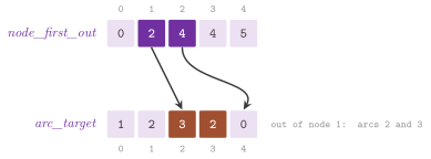
Lemma 4.4. Built from a list of \(m\) pairs
sorted by their first element, StaticDigraph has the arc \(k-1\) from \(i\) to
\(j\) for the \(k\)-th pair \((i,j)\), its OutArcIt at \(v\) visits the arcs of
indices node_first_out[v] to node_first_out[v+1]-1, and its InArcIt the
arcs into \(v\); the build takes \(O(n+m)\) time. Built from a digraph, it takes
\(O(n+\sum_v d^+(v)\log d^+(v))\) time.
Proof. The build scans the nodes \(i=0,\dots,n-1\) and, for each, consumes the
pairs whose first element is \(i\), which are consecutive in a sorted list. It
sets node_first_out[i] to the index of the first of them and gives the
consumed pairs the consecutive indices, so that the arcs out of \(i\) are the
indices between node_first_out[i] and node_first_out[i+1]-1 (an empty
range if \(i\) has none). Each arc is also put at the head of the list
node_first_in, arc_next_in of its target, which then holds the arcs into
each node. Every pair and every node is handled once, in \(O(1)\) time. From a
digraph, the nodes are numbered in one scan, and the arcs out of each node \(v\)
are collected and sorted in \(O(d^+(v)\log d^+(v))\) time before they are stored
in the same way. \(\square\)
StaticGraph. This undirected counterpart of StaticDigraph represents the
edge of index \(i\) by the arcs \(2i+1\), from \(u\) to \(v\), and \(2i\), from \(v\) to
\(u\), as SmartGraph does. Since the arcs out of each node are stored one
after the other, and the arcs into a node are the opposites of those out of
it, one array of positions serves both directions. It takes three int values
per arc (its target, its position, and the arc at each position) and one per
node, the first position of its arcs. Here the pairs of
build( n , begin , end ) may come in any order; the edge \(k-1\) has \(u\) equal
to the first element of the \(k\)-th pair and \(v\) to the second, and the arcs
are placed by a counting sort on their sources (Algorithm 4.1). A copy from a
graph numbers the nodes and the edges in the order of their iterators and then
builds from the list of the end nodes. A LEMON_ASSERT checks that the
indices of the pairs are valid.
Algorithm 4.1 (Building a StaticGraph from a list of edges).
build(n, ends[0..m-1]):
 1  for each edge i:  target[2i] = u_i ; target[2i+1] = v_i
 2  first[0..n] = 0
 3  for each edge i:  first[u_i + 1]++ ; first[v_i + 1]++
 4  for v = 0 .. n-1: first[v+1] += first[v]      (prefix sums)
 5  fill[v] = first[v] for each node v
 6  for each arc a = 0 .. 2m-1:
 7    p = fill[source(a)]++ ,  source(a) = target[a xor 1]
 8    out[p] = a ;  pos[a] = p
Here the arcs out of node \(v\) are out[first[v]] to out[first[v+1]-1],
nextOut( a ) is out[pos[a]+1] while it stays below first[v+1], and
nextIn( a ) is the opposite of nextOut on the opposite arc
(lemon/static_graph.h, StaticGraphBase::build()).
Theorem 4.1. After Algorithm 4.1, for every
node \(v\) the entries out[first[v]], ..., out[first[v+1]-1] are exactly the
arcs whose source is \(v\), in increasing order of index, and nextIn() visits
the arcs into \(v\) as the opposites of these, in the same order. The algorithm
takes \(O(n+m)\) time, and so does the copy from a graph.
Proof. The arc \(2i+1\) has target \(v_i\) and source \(\mathrm{target}[2i]=u_i\),
and the arc \(2i\) has target \(u_i\) and source \(v_i\), i.e., each edge \(i\) gives
one arc out of \(u_i\) and one out of \(v_i\) (two out of \(u_i\) if it is a loop).
Hence, after line 3 first[v+1] is \(d(v)\), and after line 4 first[v] is
\(\sum_{w<v}d(w)\), so that the intervals \([\,\)first[v]\(,\) first[v+1]\()\)
partition \(\{0,\dots,2m-1\}\) into blocks of sizes \(d(v)\). Line 7 gives the
arcs of source \(v\) the positions first[v], first[v]\(+1\), and so on, in the
order in which line 6 meets them, i.e., in increasing order of index; since
there are \(d(v)\) of them, they fill the block of \(v\). An arc \(a\) enters \(v\) if
and only if its opposite \(a\oplus 1\) leaves \(v\), and nextIn() applies
nextOut() to the opposite and takes the opposite again; hence, it visits the
arcs into \(v\) in the order of the arcs out of \(v\). Each line costs \(O(n)\) or
\(O(m)\), and the copy from a graph adds one scan of the nodes and one of the
edges. \(\square\)
abLEMON
StaticGraph is new in abLEMON (version 1.5.0): LEMON 1.3.1 had only the
static digraph. Also, the copy constructor and the assignment of
StaticDigraph are private, as those of the other structures, while in
LEMON 1.3.1 the implicit ones copied the pointers to its arrays, which
were then deleted twice.
CompactDigraph. It is a StaticDigraph without the arrays of the incoming
arcs and of the sources: it stores only node_first_out and arc_target,
i.e., one int per node and one per arc, and an Arc handle carries its
source together with its index. It is built as a StaticDigraph is (also
sorting the arcs by its own ArcLess when it copies a digraph). Its InArcIt
exists only to conform to concepts::Digraph, since with no index of the
incoming arcs it scans all the arcs. Also, arc( i ) (which is not static
here, but const) finds the source of the arc by a binary search on
node_first_out. An algorithm that visits the incoming arcs (e.g., one run on
the reverse digraph of chapter 5) should use
StaticDigraph instead.
Lemma 4.5. In CompactDigraph, arc( i ) (and
arcFromId( i )) returns the arc of index \(i\) with its source in \(O(\log n)\)
time, visiting the arcs into one node takes \(O(m)\) time, and into all the
nodes \(O(nm)\).
Proof. The array node_first_out is nondecreasing, and the arc \(i\) leaves
the node \(v\) with node_first_out[v] \(\le i<\) node_first_out[v+1]; this \(v\)
is the last index whose entry is at most \(i\), since the nodes with no arc
between \(v\) and the next node with arcs share the entry of the latter, which
is larger than \(i\). The binary search std::upper_bound finds it in \(O(\log
n)\) comparisons. firstIn() and nextIn() move along all the arcs in the
order of ArcIt and stop at those with the given target. This takes \(O(n+m)\)
time for one node, since the nodes with no arc are skipped by nextSource(),
i.e., \(O(m)\) when there is no isolated node, and \(n\) times as much for all.
\(\square\)
abLEMON
CompactDigraph comes from the repository of LEMON after its release
1.3.1, and it is distributed for the first time in abLEMON, whose
documentation also gives the cost of its InArcIt. There arc( i ) was
not const, and it could not be called on a constant digraph; the test
digraph_test calls it on one.
The program manual/examples/04-static-graphs.cc (the test
manual_04_static_graphs) builds StaticDigraph and CompactDigraph from a
sorted list of arcs and StaticGraph from a list of edges in arbitrary order.
It also copies a ListDigraph into a StaticDigraph with one of its maps and
checks that the arcs out of a node come sorted by target, and checks the
counts and the indices of the implicit graphs of the next two sections.
4.5 Full graphs¶
In lemon/full_graph.h we find FullDigraph, FullGraph and FullBpGraph,
the complete graphs, which store only their sizes and compute all the rest
from the indices; they take \(O(1)\) memory, and each of their functions takes
\(O(1)\) time. FullDigraph( n ) has the nodes \(0,\dots,n-1\) and an arc from
each node to each node, loops included, i.e., \(n^2\) arcs, the arc from \(s\) to
\(t\) having the identifier \(ns+t\). FullGraph( n ) has an edge between each
pair of distinct nodes, i.e., \(n(n-1)/2\) edges and no loop, numbered as Lemma
4.6 states. FullBpGraph( r , b ) has \(r\) red nodes (the nodes
\(0,\dots,r-1\)), \(b\) blue ones (the nodes \(r,\dots,r+b-1\)), and the \(rb\) edges
between them, the edge between the red node of index \(i\) and the blue node of
index \(j\) having the identifier \(i+rj\); the default constructors give the
empty graphs. Nodes are given by their index, as g( i ) (or g.redNode( i )
and g.blueNode( i ) in FullBpGraph), and index( v ) is the inverse.
Also, g.arc( s , t ) and g.edge( u , v ) give the arc and the edge between
two nodes, which are INVALID for \(u=v\) in FullGraph (and for two nodes of
one colour in FullBpGraph), and findArc() and findEdge() of section 4.8
use them, since the classes have the tags FindArcTag and FindEdgeTag.
FullBpGraph also has valid( item ). Finally, resize( n ) (or
resize( r , b )) changes the number of nodes; it notifies the maps that all
the items were erased and then that the new ones were built, and hence the
values of the maps are lost.
Lemma 4.6. Let \(n\ge 2\) and
\(k=\lfloor (n-1)/2\rfloor\). The map that FullGraph( n ) uses from a pair
\(u<v\) to the identifier of its edge,
is a bijection onto \(\{0,\dots,n(n-1)/2-1\}\), whose inverse writes \(e=qn+r\) with \(0\le r<n\) and returns \((q,r)\) if \(q<r\) and \((n-2-q,n-1-r)\) otherwise; the arcs of the edge \(e\) are \(2e+1\), from \(u\) to \(v\), and \(2e\).
Proof. Read \(e=qn+r\) as the cell \((q,r)\) of an array with \(n\) columns. The
first case of (4.1) takes the cells of the rows \(q<k\) above the diagonal
(\(r>q\)). The second, with \(q=n-2-u\) and \(r=n-1-v\), the cells with \(r\le q\)
(since \(v>u\) gives \(n-1-v\le n-2-u\)) of the rows \(q\le n-2-k\). Each case is
injective, and the two sets of cells are disjoint, one being above and one on
or below the diagonal. If \(n=2k+1\), then \(n-2-k=k-1\), and the rows
\(0,\dots,k-1\) are covered entirely, which gives the \(kn=n(n-1)/2\) smallest
identifiers. If \(n=2k+2\), then \(n-2-k=k\), the rows \(0,\dots,k-1\) are covered
entirely and the row \(k\) in its cells \(r\le k\), which gives the
\(kn+k+1=n(n-1)/2\) smallest identifiers. In both cases the image is an initial
segment of the right size; the inverse follows by reading the case from the
position of the cell with respect to the diagonal. The numbering of the arcs
is that of the code of arc(), source() and target(). \(\square\)
4.6 Grid and hypercube graphs¶
The headers lemon/grid_graph.h and lemon/hypercube_graph.h define two more
implicit undirected graphs, with \(O(1)\) memory, constant time counting and the
tags FindArcTag and FindEdgeTag.
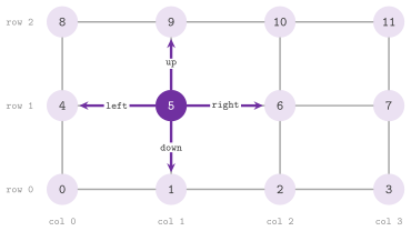
GridGraph. GridGraph( w , h ) has \(wh\) nodes, the node \((i,j)\) in column
\(i\in\{0,\dots,w-1\}\) and row \(j\in\{0,\dots,h-1\}\) having the index \(i+jw\),
and an edge between two nodes whose positions differ by 1 in one coordinate,
the vertical ones first (Figure 4.2), with the origin
at the bottom left corner. The node at a position is g( i , j ) (whose range
is checked by a LEMON_DEBUG, i.e., only when LEMON_ENABLE_DEBUG is
defined), and col( v ), row( v ) and pos( v ), a dim2::Point< int >
(cf. chapter 8), give the position of a node, while
width() and height() give the size. Also, the arcs right( v ),
left( v ), up( v ) and down( v ) leave \(v\) in the four directions, and
they are INVALID on the border. Its read maps IndexMap, ColMap and
RowMap, returned by indexMap(), colMap() and rowMap(), give the
position (a dim2::Point< int >), the column and the row of each node (e.g.,
for the coordinates of a drawing), and resize( w , h ) changes the size as
in the full graphs (we remark that the class has no default constructor).
Lemma 4.7. GridGraph( w , h ) has \(2wh-w-h\)
edges. For \(e<w(h-1)\) the edge \(e\) joins the nodes \(e\) and \(e+w\) (vertical),
and for \(e=w(h-1)+e'\) with \(0\le e'<h(w-1)\) it joins the nodes \(i+jw\) and
\(i+1+jw\), where \(j=\lfloor e'/(w-1)\rfloor\) and \(i=e'\bmod(w-1)\) (horizontal);
this numbering is a bijection between the identifiers and the pairs of
adjacent positions.
Proof. A vertical pair is \(\{(i,j),(i,j+1)\}\) with \(j<h-1\), whose lower node has index \(i+jw<w(h-1)\), and every index below \(w(h-1)\) is the lower node of exactly one such pair. Hence, \(e\mapsto\{e,e+w\}\) numbers the \(w(h-1)\) vertical pairs. A horizontal pair is \(\{(i,j),(i+1,j)\}\) with \(i<w-1\), and \((i,j)\mapsto i+j(w-1)\) is a bijection from these \(h(w-1)\) pairs onto \(\{0,\dots,h(w-1)-1\}\), whose inverse is the one in the statement. The total is \(w(h-1)+h(w-1)=2wh-w-h\). \(\square\)
HypercubeGraph. HypercubeGraph( d ), for \(d\ge 1\) (which a LEMON_ASSERT
checks), has the \(2^d\) nodes whose indices are the integers of \(d\) bits, and
an edge between two nodes whose indices differ in exactly one bit. Since the
numbers of edges and arcs are of type int, the largest dimension is 26 on a
platform with 32-bit int (since \(26\cdot 2^{26}<2^{31}\le 27\cdot 2^{27}\)).
Thus, the node of index \(i\) is g( i ) and index( v ) the inverse;
dimension() is \(d\), dimension( e ) and dimension( a ) give the bit in
which the end nodes of an edge or an arc differ, projection( v , k ) returns
whether bit \(k\) of the index of \(v\) is one, and resize( d ) changes the
dimension. Its nested read map HyperMap< T , BF = std::plus< T > > is
constructed on the graph, a range of \(d\) values \(x_0,\dots,x_{d-1}\) (whose
length a LEMON_ASSERT checks), an initial value fv (default 0) and a
binary function bf. It gives for each node the accumulation of bf over the
values of the bits that are one in its index, starting from fv, in \(O(d)\)
time; with the default function it is
\(\texttt{fv}+\sum_{k:\,\text{bit }k=1}x_k\), which gives, e.g., the position of
each node in a drawing of the hypercube from \(d\) base vectors.
Lemma 4.8. HypercubeGraph( d ) has
\(d\,2^{d-1}\) edges, the edge of identifier \(e=k\,2^{d-1}+b\), with \(0\le k<d\)
and \(0\le b<2^{d-1}\), joining the node \(u\) obtained by inserting a zero bit at
position \(k\) into \(b\) and the node \(v=u+2^k\); this numbering is a bijection,
and findEdge() computes its inverse in \(O(d)\) time.
Proof. Two indices differ only in the bit \(k\) if and only if they are \(u\)
and \(u+2^k\) with bit \(k\) of \(u\) zero. Deleting bit \(k\) from \(u\) gives a
\((d-1)\)-bit integer \(b\), and inserting a zero bit at position \(k\) into any
such \(b\) gives back a \(u\) with bit \(k\) zero. Hence, for each \(k\) the edges of
dimension \(k\) correspond one to one to the \(2^{d-1}\) values of \(b\), and
\((k,b)\mapsto k\,2^{d-1}+b\) is a bijection onto \(\{0,\dots,d\,2^{d-1}-1\}\).
Finally, findEdge( u , v ) takes \(u\oplus v\), rejects it unless it is a
single bit \(2^k\), which it finds by at most \(d\) shifts, and returns
\(k\,2^{d-1}\) plus the index \(u\) with bit \(k\) deleted. \(\square\)
4.7 Arc sets and edge sets¶
The header lemon/edge_set.h defines four structures that have their arcs (or
edges) on the nodes of another graph: ListArcSet< GR > and
SmartArcSet< GR >, which conform to concepts::Digraph, and
ListEdgeSet< GR > and SmartEdgeSet< GR >, which conform to
concepts::Graph. Their parameter GR is the type of the graph whose nodes
are shared, which may be a digraph or a graph. A set has the Node type of
GR and the nodes of GR (with their identifiers, iterators and notifier),
and only the arcs or edges belong to it. Hence, several sets may be built on
one graph (e.g., the arcs of several commodities, or a sparse subgraph whose
arcs are not in the graph), and the node maps of GR serve all of them. A set
is constructed on the graph, ListArcSet< GR > s( g ), and it has
addArc( s , t ) (or addEdge( u , v )), clear(), and the functions of its
concept; its counting is linear.
Both List sets link the arcs of each node in doubly linked lists, as
ListDigraph and ListGraph do, and they also have erase( a ) (or
erase( e )). They observe the nodes of the underlying graph, through a
protected node map of the nested class NodesImpl; when a node is erased from
it, they erase its arcs first, and when the graph is cleared they clear
themselves. The two Smart sets store the arcs in a vector with singly linked
lists, which is slightly faster, and cannot erase them. They observe the nodes
too, but an erased node that has an arc in the set invalidates the whole set
(by the exception ImmediateDetach of appendix
A), which can no longer be used; their function
valid() returns whether this has not happened. An erased node with no arc in
the set leaves it valid.
abLEMON
The functions eraseNode() and clearNodes(), by which the observer of
the nodes updates a set, and that observer itself are protected in all
four sets; in LEMON 1.3.1 they were public in the List sets, so that a
call could erase the arcs of a node still in the graph, or all the arcs.
The test edge_set_test checks that no set exposes the two functions.
Lemma 4.9. In the List sets, addArc() (or
addEdge()) takes \(O(1)\) amortized time, erase( a ) (or erase( e ))
\(O(1)\) time, and the erasure of a node of the underlying graph \(O(1)\) time
plus \(O(1)\) for each arc of the set at the node; in the Smart sets,
addArc() (or addEdge()) takes \(O(1)\) amortized time, and the erasure of a
node of the underlying graph \(O(1)\) time.
Proof. The arcs are kept in a vector with a free list (the List sets) or
appended to it (the Smart sets), and linked at the head of the lists of
their ends, as in Lemma 4.1. The List sets unlink an arc in \(O(1)\) time from
its doubly linked lists, and erase the arcs at an erased node one by one from
the heads of its lists. The Smart sets only test whether the lists of the
erased node are empty, in \(O(1)\) time, and detach themselves otherwise.
\(\square\)
The program of section 4.9 builds a ListEdgeSet and a SmartArcSet on a
ListDigraph, and checks both behaviors.
4.8 Counting and finding arcs¶
Counting. In lemon/core.h, the functions countNodes( g ),
countArcs( g ), countEdges( g ), countRedNodes( g ) and
countBlueNodes( g ) return the number of items of a kind. They call
nodeNum(), arcNum(), edgeNum(), redNum() or blueNum() if the
structure defines the corresponding tag (NodeNumTag, ArcNumTag,
EdgeNumTag; NodeNumTag also selects redNum() and blueNum()), and count
the items with an iterator otherwise, whereas countItems< GR , Item >( g )
always iterates. The choice is made at compile time by the helper classes
CountNodesSelector, CountArcsSelector, CountEdgesSelector,
CountRedNodesSelector and CountBlueNodesSelector of the internal namespace
_core_bits of lemon/core.h, specialized by enable_if on the tag, which a
user does not call directly. Similarly, countOutArcs( g , v ),
countInArcs( g , v ) and countIncEdges( g , v ) iterate on the arcs or
edges at a node, through the template
countNodeDegree< GR , DegIt >( g , v ), which counts the items of any
incidence iterator DegIt.
Finding the arcs between two nodes. A call
findArc( g , u , v , prev = INVALID ) returns an arc from u to v, the
first one if prev is INVALID and the one after prev otherwise, or
INVALID if there is none; repeated calls, each with the previous result,
enumerate the parallel arcs. On a structure with the tag FindArcTag (the
full, grid and hypercube graphs) it calls g.findArc(), and on the others it
scans the arcs out of u. An iterator ConArcIt< GR >, constructed as
ConArcIt< GR > a( g , u , v ), wraps the same enumeration, and
ConArcIt< GR >( g , a ) continues it from the arc a. For undirected
graphs, findEdge( g , u , v , prev = INVALID ) and ConEdgeIt< GR > find
the edges between u and v (in either orientation) by scanning the edges at
u, or by g.findEdge() with FindEdgeTag. Each loop at u is returned
once for \(u=v\), and ConEdgeIt< GR >( g , e ) continues the enumeration from
the edge e, on the edges between its two ends. The two functions dispatch on
the tags through the internal classes FindArcSelector and
FindEdgeSelector.
abLEMON
ConEdgeIt constructed from an edge continues on the edges between the
two ends of that edge; in LEMON 1.3.1 it left its two nodes INVALID, and
its operator++ searched the edges between two INVALID nodes. The test
graph_utils_test counts the parallel edges after one.
Lemma 4.10. (i) Without the tags, the counting
functions take \(O(n)\), \(O(m)\) (or the number of edges) and \(O(d^+(v))\),
\(O(d^-(v))\), \(O(d(v))\) time, and with them \(O(1)\) time. (ii) Without
FindArcTag, the calls \(a_1=\) findArc( g , u , v ), \(a_{i+1}=\)
findArc( g , u , v , a_i ) return each arc from u to v exactly once, in
the order of OutArcIt at u, and then INVALID, in \(O(d^+(u))\) time in
all. (iii) Without FindEdgeTag, findEdge() does the same for the edges
between u and v, each loop once, in \(O(d(u))\) time in all.
Proof. (i) Each iteration visits each item once (it is the contract of the
iterators, cf. appendix A), and a counter is
increased in \(O(1)\) per item; the tagged functions return a stored number.
(ii) The first call starts at firstOut( e , u ), and each call resumes from
the successor of prev in the list of the arcs out of u. Each call moves
along that list until an arc with target v or the end, so that the arcs out
of u are visited once over all the calls, and every arc from u to v is
returned when it is met. (iii) For \(u\ne v\) the scan follows the incidences of
u by firstInc() and nextInc() and stops at the edges whose other end is
v. In it, the direction flag of prev is recomputed as whether u is its
first end; for \(u=v\) it stops only at the incidences with the flag true and
the other end u, which a loop has once of its two. The incidences of u are
\(d(u)\), each visited once. \(\square\)
Look-up structures. When many arcs are looked for in one digraph, three
classes of lemon/core.h answer faster than the scan, at the price of some
memory and of a preprocessing. They are queried by operator(), as in
ArcLookUp< GR > look( g ) followed by look( s , t ).
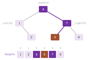
ArcLookUp< GR >builds, for each node, a binary search tree of the arcs out of it, keyed by their targets under the order<of the nodes (the order of the identifiers, in the structures of this chapter; Figure 4.3). Its constructor callsrefresh(), which builds all the trees, andrefresh( v )rebuilds the tree of one node. A querylook( s , t )returns an arc fromstot, orINVALID. It finds one arc only. The structure is static: after a change of the digraphrefresh()must be called (orrefresh( v ), if only the arcs out ofvchanged) before the next query.AllArcLookUp< GR >is anArcLookUpthat also links the arcs with the same source and target, andlook( s , t , prev = INVALID )enumerates them: the first ifprevisINVALID, the one afterprevotherwise. It is static as well; itsrefresh( v )andrefresh()rebuild the trees and the links.DynArcLookUp< GR >keeps a self-adjusting binary search tree, the splay tree of Sleator and Tarjan 1985, for the arcs out of each node, and it observes the arcs of the digraph, so that it follows each addition and erasure with no refresh (a build or a clear of the digraph rebuilds or empties it). A querylook( s , t , p = INVALID )enumerates the arcs fromstotas the one ofAllArcLookUpdoes. However, as the header remarks, its constant factors are often larger than those of the two static classes, which are therefore preferable on a digraph that changes rarely.
The trees of ArcLookUp are built by Algorithm 4.2: refresh( v ) sorts the
arcs out of v (by its private comparator ArcLess) and makes the middle one
the root of each subtree.
Algorithm 4.2 (The search tree of ArcLookUp).
refresh(v):
 1  L = the arcs out of v, sorted by their target
 2  head[v] = build(L, 0, |L|-1)          (INVALID if L is empty)
build(L, a, b):
 3  m = (a + b) / 2
 4  left[L[m]]  = build(L, a, m-1) if a < m, else INVALID
 5  right[L[m]] = build(L, m+1, b) if m < b, else INVALID
 6  return L[m]
lookup(s, t):                             (operator()(s, t))
 7  e = head[s]
 8  while e != INVALID and target(e) != t:
 9    e = left[e] if t < target(e) else right[e]
10  return e
Theorem 4.2. The tree that Algorithm 4.2 builds
on \(k\) arcs is a binary search tree on their targets of height
\(\lceil\log_2(k+1)\rceil\), whose in-order is the sorted order \(L\). Hence, a
query look( s , t ) returns an arc from s to t if there is one, and
INVALID otherwise, after following at most \(\lceil\log_2(d^+(s)+1)\rceil\)
arcs of the tree; refresh( v ) takes \(O(d^+(v)\log d^+(v))\) time and
refresh() \(O(n+m\log\Delta)\) time.
Proof. By induction on \(k=b-a+1\), build( L , a , b ) returns a tree whose
in-order is \(L[a..b]\): the root is \(L[m]\), its left subtree has the in-order
\(L[a..m-1]\) and its right one \(L[m+1..b]\). Since \(L\) is sorted, every target
in the left subtree is not larger, and every target in the right one is not
smaller, than the target of the root, which is the property of a binary search
tree. The subtrees have \(\lfloor (k-1)/2\rfloor\) and \(\lfloor k/2\rfloor\)
arcs, so that the height satisfies \(h(0)=0\) and
\(h(k)=1+h(\lfloor k/2\rfloor)\); if \(2^{j-1}<k+1\le 2^j\), then
\(2^{j-2}<\lfloor k/2\rfloor+1\le 2^{j-1}\), and \(h(k)=\lceil\log_2(k+1)\rceil\)
follows by induction on \(j\). The query of lines 7 to 10 follows one path from
the root, going left when \(t\) is smaller than the target of the current arc
and right otherwise; by the search tree property, an arc with target \(t\), if
any, lies on that path, and the path has at most \(h(d^+(s))\) arcs. The sort
dominates the cost of refresh( v ), and refresh() calls it for every node,
with \(\sum_v d^+(v)\log d^+(v)\le m\log\Delta\). \(\square\)
Lemma 4.11. In AllArcLookUp, the calls
\(a_1=\) look( s , t ), \(a_{i+1}=\) look( s , t , a_i ) return each arc from
s to t exactly once and then INVALID; the first call takes
\(O(\log d^+(s))\) time and each of the others \(O(1)\).
Proof. By Theorem 4.2 the arcs from s to t are consecutive in the
in-order of the tree of s. The first call descends as in Algorithm 4.2 until
an arc with target \(t\). Then it keeps descending, to the left from each arc
with target \(t\) (recording it) and to the right from the others; the last arc
recorded is the first of the consecutive ones in the in-order, and the path
has at most \(\lceil\log_2(d^+(s)+1)\rceil\) arcs. After the trees are built,
refresh visits each tree in reverse in-order and sets the link next of
each arc to its in-order successor if this has the same target, and to
INVALID otherwise; the next calls follow these links, in \(O(1)\) each,
through the consecutive arcs with target \(t\). \(\square\)
Theorem 4.3. In DynArcLookUp, consider a
sequence of \(q\) operations on the tree of one node \(s\) with at most \(d\) arcs,
each of which is an addition or an erasure of an arc of the digraph, or a
first query look( s , t ). Its total time is \(O(d\log d+q\log d)\), i.e.,
\(O(\log d)\) amortized per operation. Furthermore, a first query
look( s , t ) splays the arc \(x_t\) that ends its search path, which is the
leftmost arc with target at least \(t\) or the rightmost one with target smaller
than \(t\); for a sequence of first queries in which the arc \(a\) is splayed
\(q_a\ge 1\) times, the total time is \(O(d\log d+\sum_a q_a(1+\log(q/q_a)))\),
i.e., within a constant factor of the best static search tree for these
frequencies.
Proof sketch. Each operation either costs \(O(1)\) or follows a path from the
root and then splays the last node of the path, i.e., moves it to the root by
the rotations zig, zig-zig and zig-zag of the function splay(). An addition
inserts the arc as a leaf and splays it. An erasure costs \(O(1)\) when the arc
has at most one child, or when its left child has no right one, and otherwise
replaces the arc by its in-order predecessor and splays the old parent of the
predecessor. A first query descends to the left at the arcs with target at
least \(t\) and to the right at the others, and splays the last arc visited,
which is therefore one of the two in-order neighbours of the boundary between
the targets smaller than \(t\) and the others. With the potential
\(\Phi=\sum_a\log_2 s(a)\), where \(s(a)\) is the size of the subtree of \(a\), the
access lemma of Sleator and Tarjan 1985, Lemma
1 bounds the amortized cost
of splaying a node at the end of a path by \(3\log_2 d+1\) (the path being paid
by the rotations), and an erasure does not increase \(\Phi\), since every
subtree size it changes decreases. The initial potential of the balanced trees
of refresh() is at most \(d\log_2 d\), which gives the first bound (the
balance theorem, ibid., Theorem 1); with the weights \(q_a/q\) in place of the
unit ones, the same lemma gives the second (the static optimality theorem,
ibid., Theorem 2). \(\square\)
We remark that Theorem 4.3 does not cover the next queries
look( s , t , p ). Such a query takes the in-order successor of \(p\) and
splays it; when \(p\) has a right subtree, the successor is the leftmost arc of
that subtree, and the descent to it is paid by the splay, while otherwise the
query climbs from \(p\) to the successor, an ancestor of \(p\), and this climb is
not paid by the splay of the ancestor (nor is the climb to the root when \(p\)
has no successor). Hence, a next query takes \(O(h+\log d)\) amortized time,
where \(h\le d\) is the depth of \(p\) in the tree, and the bound \(O(\log d)\) that
the header gives for the first queries does not extend to it. The program
manual/examples/04-arc-lookup.cc (the test manual_04_arc_lookup) compares
the four ways of finding an arc on a digraph with parallel arcs, enumerates
the three parallel arcs by findArc(), ConArcIt, AllArcLookUp and
DynArcLookUp, and shows that only DynArcLookUp sees a new arc before a
refresh.
abLEMON
AllArcLookUp::refresh(), the variant without arguments, calls
refresh( n ) for each node; in LEMON 1.3.1 it passed an arc to
refresh( Node ) and did not compile. The test graph_utils_test and the
program manual/examples/04-arc-lookup.cc call it.
4.9 Copying graphs¶
Since a graph structure cannot be copied by its copy constructor, its
duplicate, possibly into a structure of another type, is made by the classes
DigraphCopy< From , To >, GraphCopy< From , To > and
BpGraphCopy< From , To > of lemon/core.h, or by the functions
digraphCopy( from , to ), graphCopy( from , to ) and
bpGraphCopy( from , to ), which return such an object. Before running it one
can request the following data, each by a function that returns the object (so
that the requests can be chained).
nodeRef( map ), a map with the nodes offromas keys, into which the copy writes the image of each node, andnodeCrossRef( map ), a map with the nodes oftoas keys, into which it writes the original of each node;arcRef(),arcCrossRef(),edgeRef(),edgeCrossRef(),redRef(),redCrossRef(),blueRef()andblueCrossRef()do the same for the other kinds of items;nodeMap( fmap , tmap ), which copies the values of the mapfmapoffrominto the maptmapofto, item by item;arcMap(),edgeMap(),redNodeMap()andblueNodeMap()do the same for the other kinds of items;node( n , tn ), which writes intotnthe image of the noden, andarc(),edge(),redNode()andblueNode()likewise.
Then run() clears to and copies the structure, followed by the data that
were requested (Algorithm 4.3). Internally, each request is an object of one
of the classes MapCopy, ItemCopy, RefCopy and CrossRefCopy (derived
from MapCopyBase), and the structure is copied by DigraphCopySelector,
GraphCopySelector or BpGraphCopySelector, which call build() on a target
with BuildTag. Also, GraphCopy and BpGraphCopy compute the images of the
arcs (and BpGraphCopy those of the nodes, from the red and the blue ones) on
demand, by their private maps ArcRefMap and NodeRefMap. In GraphCopy the
image of an arc is the arc of the image of its edge whose source is the image
of its source (for a loop, the arc with the same direction()), so that the
orientation of each arc is kept even if the target structure orders the end
nodes of its edges differently.
Algorithm 4.3 (DigraphCopy::run()).
run():
 1  nr = node map of from, ar = arc map of from      (local references)
 2  if To has BuildTag:  to.build(from, nr, ar)
 3  else:
 4    to.clear()
 5    for each node v of from:  nr[v] = to.addNode()
 6    for each arc a of from:   ar[a] = to.addArc(nr[source(a)], nr[target(a)])
 7  for each requested node datum:  copy it through nr
 8  for each requested arc datum:   copy it through ar
Theorem 4.4. After DigraphCopy::run(), nr
is a bijection from the nodes of from onto those of to and ar one from
the arcs, with
\(\mathrm{source}(\mathrm{ar}[a])=\mathrm{nr}[\mathrm{source}(a)]\) and
\(\mathrm{target}(\mathrm{ar}[a])=\mathrm{nr}[\mathrm{target}(a)]\) for every
arc \(a\); the requested data are the images of those of from under these
bijections. The copy takes \(O(n+m)\) time plus the time of the data requested,
except when the target is built by build(), whose cost is that of section
4.4 (e.g., \(O(n+\sum_v d^+(v)\log d^+(v))\) for a StaticDigraph). The same
holds for GraphCopy and BpGraphCopy with the edges, and with the red and
blue nodes.
Proof. Without BuildTag, to is cleared, and each node of from gets a
new node (distinct, since they are added one by one). Each arc a new arc
between the images of its ends, which gives the two bijections and the
relation of the ends; each addition takes \(O(1)\) amortized time on the
structures of this chapter. With BuildTag, build() writes the same maps by
Lemma 4.4 and Theorem 4.1 (whose copies from a graph keep the end nodes of
each edge). A reference, a cross reference, a map or an item is then copied by
one pass over the items of its kind (or one access) through nr or ar. In
GraphCopy, the image of an arc is computed in \(O(1)\) from the image of its
edge, as described above. The node references are always computed, because the
arcs need them. \(\square\)
abLEMON
DigraphCopy, GraphCopy and BpGraphCopy hold the objects that copy
the requested data, which their destructor deletes; in abLEMON they have a
move constructor and no copy constructor, which digraphCopy() and the
other functions use to return them by value. LEMON 1.3.1 copied them, and
a copy that was not elided deleted those objects twice.
The program manual/examples/04-copy-and-sets.cc (the test
manual_04_copy_and_sets) copies a ListGraph with a loop into a nonempty
SmartGraph. It requests the node references, the cross references of the
edges, an edge map and the image of one backward arc; then it builds a
ListEdgeSet and a SmartArcSet on a ListDigraph, and checks that erasing
a node of the underlying digraph erases its edges from the first and
invalidates the second.
4.10 Exercises¶
Exercise 4.1. Build a ListDigraph with \(10^5\)
nodes and \(10^6\) random arcs, and measure the time of a loop that visits the
arcs out of each node, on it and on the StaticDigraph obtained by
digraphCopy(). Explain the difference by the storage of Figure
4.1. (The test test/digraph_test.cc checks that the
two structures have the same arcs.)
Exercise 4.2. Find, from the code of
ListDigraph::contract(), which arcs contract( u , v ) with r = true
erases and which loops at u it keeps, and write the sequence of calls that
contracts u and v and erases all the loops at u. (The program
manual/examples/04-list-graph.cc contracts two nodes.)
Exercise 4.3. Modify Algorithm 4.1 so that the
arcs out of each node come sorted by the index of their target, still in
\(O(n+m)\) time, and prove it as Theorem 4.1 is proved. (The test
test/graph_test.cc checks a StaticGraph built from a random graph with
loops and parallel edges.)
Exercise 4.4. Prove that FullBpGraph( r , b )
numbers its edges bijectively by \(i+rj\), as Lemma 4.6 does for FullGraph,
and check the formulae of Lemmas 4.6 to 4.8 against nodeNum(), edgeNum()
and arcNum() and against findEdge() for small sizes. (The program
manual/examples/04-static-graphs.cc checks some of them.)
Exercise 4.5. On a digraph with \(n\) nodes and \(m\)
arcs, compare the total time of \(q\) queries by findArc(), by ArcLookUp
(preprocessing included) and by DynArcLookUp, and find, by Lemma 4.10 and
Theorems 4.2 and 4.3, the values of \(q\) above which each look-up structure
becomes the faster choice. (The program manual/examples/04-arc-lookup.cc and
the test test/arc_look_up_test.cc use the three structures.)
Exercise 4.6. Copy a ListBpGraph into a
SmartBpGraph with bpGraphCopy(), requesting the references of the red
nodes and a blue node map, and check that each edge keeps its red and its blue
end. (The test test/graph_copy_test.cc copies bipartite graphs.)