10. Shortest paths¶
We are concerned in this chapter with the shortest paths of a digraph
\(G=(N,A)\), with \(n=|N|\) nodes and \(m=|A|\) arcs, whose arcs have lengths
\(\ell : A\to\mathbb{R}\). The library has five classes for them. Dijkstra
(lemon/dijkstra.h) computes the shortest paths from a set of sources when
the lengths are nonnegative, and BidirDijkstra and AStar
(lemon/bidir_dijkstra.h, lemon/astar.h) compute a shortest path between
two nodes, usually scanning much less of the digraph. BellmanFord
(lemon/bellman_ford.h) accepts negative lengths and detects the negative
cycles, and Suurballe (lemon/suurballe.h) finds \(k\) arc-disjoint paths of
least total length between two nodes. We first state the problem and the
optimality conditions that all of them rely on (§10.1), and then
describe the classes in this order.
10.1 The problem and its optimality conditions¶
As in §8.1, a path is a sequence of arcs \(P=(a_1,\dots,a_k)\), each starting where the previous one ends (so that a node may repeat), and we call it simple if no node repeats. Its length is \(\ell(P)=\sum_{i=1}^k \ell(a_i)\), and, given a source \(s\), the distance of a node \(v\) is
with \(d(v)=+\infty\) if \(v\) cannot be reached from \(s\). If no cycle of negative length can be reached from \(s\), removing the cycles of a path does not make it longer, and the infimum is the minimum over the (finitely many) simple paths; otherwise, \(d(v)=-\infty\) for each node \(v\) reachable from such a cycle. With several sources \(S\), each with an initial distance \(d_0(s)\), the distance of \(v\) is the least value of \(d_0(s)+\ell(P)\) over the sources \(s\) and the paths \(P\) from \(s\) to \(v\), i.e., the distance (10.1) from a new source joined to each \(s\in S\) by an arc of length \(d_0(s)\). All the classes of this chapter maintain tentative distances \(d\) and a predecessor arc for each node, and stop when the following conditions hold.
Theorem 10.1. Let \(d\) be finite on the nodes reachable from \(s\), with \(d(s)=0\), and let \(d(v)\) be the length of some path from \(s\) to \(v\) for each of them. Then \(d\) is the distance (10.1) if and only if
If, moreover, each node \(v\neq s\) has a predecessor arc \(uv\) with \(d(v)=d(u)+\ell(uv)\), and following the predecessor arcs back from each node leads to \(s\), these arcs form a tree of shortest paths.
Proof. If (10.2) holds, summing it along any path \(P\) from \(s\) to \(v\) gives \(d(v)\le d(s)+\ell(P)=\ell(P)\); since \(d(v)\) is itself the length of a path, it is the minimum (10.1). Conversely, if \(d\) is the distance and is finite, appending the arc \(uv\) to a path of length \(d(u)\) gives a path to \(v\) of length \(d(u)+\ell(uv)\), which is at least \(d(v)\). For the tree, the path of predecessor arcs from \(s\) to \(v\) has length \(d(v)\), by summing the equalities along it, and is therefore a shortest path. Since it reaches \(s\) from each node, the arcs have no cycle and form a tree. \(\square\)
Equivalently, (10.2) means that the reduced lengths
are nonnegative for the potential \(\pi=d\). Since \(\ell_\pi(P)=\ell(P)+\pi(u)-\pi(v)\) for any path \(P\) from \(u\) to \(v\), a change of the lengths into reduced lengths changes the length of all the paths between two given nodes by the same amount, and keeps the shortest ones. We shall use this fact for A* (§10.3) and for Suurballe's algorithm (§10.5). Also, the shortest path problem is the minimum cost flow problem of chapter 13 in which one unit of flow is sent from \(s\) to each other node, and \(d\) is an optimal potential of its dual.
Table 10.1. The classes of this chapter, with
the lengths they accept and the cost of a run on a digraph of \(n\) nodes and
\(m\) arcs (\(k\) is the number of paths of Suurballe).
| class | lengths | answers | time with the default heap |
|---|---|---|---|
Dijkstra |
\(\ge 0\) | all the distances from a set of sources | \(O((n+m)\log n)\) |
BidirDijkstra |
\(\ge 0\) | one path between two nodes | \(O((n+m)\log n)\), usually much less |
AStar |
\(\ge 0\) | one path between two nodes, with a heuristic | \(O((n+m)\log n)\) with a consistent heuristic |
BellmanFord |
any | all the distances, or a negative cycle | \(O(nm)\) |
Suurballe |
\(\ge 0\) | \(k\) arc-disjoint paths between two nodes | \(O(k\,(n+m)\log n)\) |
10.2 Dijkstra's algorithm¶
In the algorithm of Dijkstra 1959,
the reached nodes that are not yet processed are kept in a heap \(H\), keyed by
their tentative distance. At each step it removes a node of least tentative
distance, declares its distance final, and relaxes its out-arcs, i.e., it
decreases the tentative distance of each target \(v\) of an arc \(uv\) to
\(d(u)+\ell(uv)\) if this is smaller (Algorithm 10.1). In the class, the sum and
the comparison are the members plus() and less() of an object of
operation traits, and the initial distance of a source is zero() unless
given; we write them \(\oplus\) and \(\prec\), and \(\preceq\) for "not \(\succ\)".
Algorithm 10.1 (Dijkstra's algorithm,
Dijkstra).
init():
1  for each node v: pred(v) := INVALID; processed(v) := false; v has never been in H
addSource(s, d0):
2  if s has never been in H: push s on H with priority d0
3  else if s is in H and d0 < priority(s): decrease it to d0; pred(s) := INVALID
processNextNode():
4  u := the node of least priority in H; d(u) := its priority; pop u; processed(u) := true
5  for each arc a = uv out of u:
6     if v was never in H: push v with priority d(u) + l(a); pred(v) := a
7     else if v is in H and d(u) + l(a) < priority(v):
8        decrease the priority of v to d(u) + l(a); pred(v) := a
9  return u
start():   while H is not empty: processNextNode()
In the theorem below, the value of a path \(P=(a_1,\dots,a_k)\) from a source \(s\) is \(d_0(s)\oplus\ell(a_1)\oplus\cdots\oplus\ell(a_k)\), computed from the left. The distance \(d(v)\) is the least value of a path from a source to \(v\); with the default operations it is the distance of §10.1.
Theorem 10.2. Suppose that \(\preceq\) is a
total preorder (that of the heap too), and that, for each arc \(a\) and all the
values \(x\preceq y\), one has \(x\preceq x\oplus\ell(a)\) and
\(x\oplus\ell(a)\preceq y\oplus\ell(a)\); with the default operations, this
means that the lengths are nonnegative. Then each node processed by Algorithm
10.1 has its distance from the sources as its priority when it leaves the
heap, and the predecessor arcs of the processed nodes form a forest of
shortest paths. The algorithm performs at most \(n\) pushes and pops and at most
\(m\) decreases of a priority (plus one per call of addSource()).
Proof. Each priority is the value of a path (by steps 2, 6 and 8), and therefore not smaller than the distance of its node. By the two hypotheses, removing a cycle from a path does not increase its value, so that each distance is the value of a simple path. We show by induction on the order of processing that the priority \(p(u)\) of the node \(u\) processed in step 4 is at most \(d(u)\). Let \(P\) be a simple path of value \(d(u)\) from a source \(s\), and let \(y\) be its first node that is not processed before \(u\) (it exists, since \(u\) is not). If \(y=s\), its priority is at most \(d_0(s)\), by steps 2 and 3. If not, its predecessor \(x\) on \(P\) was processed with \(p(x)=d(x)\), which is at most the value of the part of \(P\) up to \(x\). When \(x\) was processed, steps 6 to 8 gave \(y\) a priority at most \(p(x)\oplus\ell(xy)\), i.e., by the second hypothesis, at most the value of the part of \(P\) up to \(y\). By the first hypothesis, the value does not decrease along the rest of \(P\); hence, \(p(y)\preceq d(u)\), and \(p(u)\preceq p(y)\) since \(u\) leaves the heap first (or \(u=y\)). The predecessor of a processed node \(v\) is the arc \(xv\) that gave \(v\) its final priority, from a node \(x\) processed before \(v\), with \(d(v)=d(x)\oplus\ell(xv)\); hence, the path of predecessor arcs reaches a source, and its value is \(d(v)\). Finally, each node enters the heap once, and each arc is relaxed once, from its source. \(\square\)
The time therefore depends on the heap (cf. chapter 7).
With the BinHeap of the default traits, all the operations take \(O(\log n)\)
and the search takes \(O((n+m)\log n)\), while a FibHeap gives \(O(m+n\log n)\)
by its decreases in amortized \(O(1)\) (Fredman and Tarjan
1987). Note that the Fibonacci
bound is better only in theory for most digraphs of practical size, the binary
heap (or the 4-ary QuadHeap) being usually faster; with small integer
lengths, a RadixHeap or a BucketHeap is perhaps worth a try. For instance,
\(\oplus\) defined as the maximum (with nonnegative lengths) satisfies the
hypotheses of Theorem 10.2, and gives the paths of least bottleneck, i.e., the
paths whose longest arc is as short as possible. Note that the heap still
orders the priorities by the comparison of its own type (std::less in the
default traits), which must agree with less().
Template parameters and traits. Dijkstra< GR , LEN , TR > takes the
digraph type GR (ListDigraph by default), the type LEN of the map of the
lengths (by default GR::ArcMap< int >), whose Value is the type of the
distances, and the traits class TR, by default
DijkstraDefaultTraits< GR , LEN >. These traits give Digraph, LengthMap,
Value, OperationTraits, i.e., the operations on the distances (by default
DijkstraDefaultOperationTraits< Value >, with the static zero(), plus()
and less() that are the zero, the sum and the comparison of the type), and
HeapCrossRef and Heap, i.e., a NodeMap< int > and a BinHeap with
std::less. They also give the three maps PredMap (a NodeMap< Arc >),
DistMap (a NodeMap of the distances) and ProcessedMap (a NullMap),
each with a function create...(). Named parameters SetPredMap< T >,
SetDistMap< T >, SetProcessedMap< T > and SetStandardProcessedMap change
the maps as in §9.1. Moreover, SetHeap< H , CR >
sets the types of the heap and of its cross reference map, both of which must
then be given by heap(); SetStandardHeap< H , CR > sets them for a heap
that the algorithm can allocate (one whose constructor takes the cross
reference map, which takes the digraph). Finally, SetOperationTraits< T >
replaces the operations. The class also defines Traits, Path (the type of
the path dumper of path()) and Create.
abLEMON
Dijkstra (and BellmanFord, §10.4) keep an object of their
operation traits class, default constructed or given by
operationTraits( ops ), and call its members plus() and less();
hence, the operations may depend on the instance, e.g., on a tolerance
stored in the object. In LEMON 1.3.1 they were static functions of the
traits class.
Interface. Its constructor takes the digraph and the length map, and its
setters are lengthMap( m ), operationTraits( ops ) (with the reader
operationTraits()), predMap( m ), distMap( m ), processedMap( m ) and
heap( hp , cr ); the maps and the heap not given are allocated by init()
and deleted by the destructor. Its execution control is made of init(),
addSource( s , dst ), processNextNode(), nextNode(), emptyQueue() and
queueSize(), the three forms of start(), and run( s ) and
run( s , t ). A call addSource( s , dst ) adds a source with the initial
distance dst (zero() by default), by steps 2 and 3 of Algorithm 10.1.
Hence, a source added twice keeps the smaller of its two distances, and a node
already processed is left as it is.
abLEMON
In LEMON 1.3.1, addSource( s , dst ) raised the priority of a source
already in the heap with a smaller one to dst, and pushed again a node
already processed; the test dijkstra_test adds sources twice.
Then start() processes the nodes until the heap is empty, while start( t )
processes them until t is on the top of the heap, then writes the distance
of t, marks it processed and pops it without relaxing its arcs. Also,
run( s , t ) does init(), addSource( s ) and start( t ), and returns
whether t was processed. Similarly, start( nm ) stops when a node with
nm true is on the top of the heap, writes its distance and marks it
processed (in the ProcessedMap, while it stays in the heap), and returns it,
or returns INVALID if the heap empties first. By Theorem 10.2, the distance
of the node at which these searches stop is final.
Its queries are dist( v ), predArc( v ), predNode( v ), path( t ) (a
path dumper, cf. §8.1), distMap(), predMap(),
reached( v ) (whether \(v\) has been in the heap) and processed( v )
(whether it has left it). The distance is written into the DistMap only when
a node is processed; hence, dist( v ) is undefined for a node that is
reached but not processed, and for such a node, currentDist( v ) returns its
priority in the heap, i.e., an upper bound on its distance that may still
decrease.
Function-type interface. Finally, dijkstra( g , length ) returns a
DijkstraWizard, whose named function parameters are predMap( m ),
distMap( m ), processedMap( m ), path( p ) and dist( d ), and whose
runs are run( s ) and run( s , t ). The latter returns whether t is
reached and fills the path and the distance, as in
§9.4; the base class DijkstraWizardBase holds the
parameters, and DijkstraWizardDefaultTraits their default types.
The program manual/examples/10-dijkstra.cc (the test manual_10_dijkstra)
runs Dijkstra's algorithm on a grid and checks the distances against (10.2).
Then it uses two sources, the function-type interface and the operations of
the least bottleneck, and compares the results with those of the two
point-to-point searches of the next section.
10.3 Shortest paths between two nodes¶
When only the path from a source \(s\) to a target \(t\) is wanted,
Dijkstra::run( s , t ) stops when \(t\) is processed, but it still processes
all the nodes closer to \(s\) than \(t\). Both classes of this section usually
scan far fewer nodes. Both have nonnegative lengths, and both answer any
number of queries with one object, each by a call run( s , t ) that returns
whether \(t\) is reachable from \(s\). Both give the result by dist() and
path() (a lemon::Path, empty when \(s=t\)), with the sums and the
comparisons of the type of the lengths. Their node maps are allocated once, by
the constructor; each run resets only the nodes that the previous run touched,
and its time is therefore proportional to the part of the digraph that it
scans (times the logarithm of the size of the heap). Their heap is a BinHeap
by default. The named parameter SetHeap< H , CR > replaces it by a heap of
type H with a cross reference map of type CR (a NodeMap< int > by
default), as in SetHeap< FibHeap< int , IntNodeMap > >::Create.
abLEMON
BidirDijkstra and AStar are new in abLEMON (from trac #249 and #376 of
LEMON), and take the type of their heap from a traits class
(BidirDijkstraDefaultTraits, AStarDefaultTraits) through SetHeap.
Bidirectional search. BidirDijkstra< GR , LEN , TR > runs two searches
of Dijkstra (Pohl 1971), a
forward one from \(s\) along the arcs and a backward one from \(t\) against them,
with tentative distances \(d_f\) and \(d_b\) and heaps \(H_f\) and \(H_b\). At each
step it advances the search whose least priority is smaller (the forward one
on a tie). Each arc \(uv\) scanned by one search whose other end has been seen
by the other search gives a path from \(s\) to \(t\), of length
\(d_f(u)+\ell(uv)+d_b(v)\), and the algorithm keeps the shortest one found, of
length \(\mu\), with the arc \(\mathit{meet}\) that gave it. Writing \(\min H\) for
the least priority in \(H\) (\(+\infty\) for an empty heap), it stops as soon as
(Algorithm 10.2, in which a node is seen by a search once it has entered its heap, and done once it has left it).
Algorithm 10.2 (Bidirectional Dijkstra,
BidirDijkstra::run( s , t )).
1  if s = t: return true with the empty path
2  push s on Hf and t on Hb with priority 0; found := false
3  while Hf and Hb are not empty:
4     if found and min(Hf) + min(Hb) >= mu: stop
5     X := the forward search if min(Hf) <= min(Hb), else the backward one; Y := the other
6     u := pop the top of X
7     for each arc a of u (out-arcs if X is forward, in-arcs if backward), w its other end:
8        relax w in X with d_X(u) + l(a), as in Algorithm 10.1 (unless w is done in X)
9        if w has been seen by Y and (not found or d_X(u) + l(a) + d_Y(w) < mu):
10          found := true; mu := d_X(u) + l(a) + d_Y(w); meet := a
11 if not found: return false
12 path := the forward tree to the tail of meet, meet, the backward tree from its head
Theorem 10.3. With nonnegative lengths,
BidirDijkstra::run( s , t ) returns false if and only if \(t\) is not
reachable from \(s\); otherwise, \(\mu\) is the distance \(\delta(s,t)\) from \(s\) to
\(t\), and the path built at step 12 has length \(\mu\). Each node is pushed and
popped at most once by each search, and each arc relaxed at most once by
each.
Proof. Each search is a search of Dijkstra, interrupted at times. Hence, by
Theorem 10.2, a node done by the forward search has \(d_f\) equal to its
distance from \(s\), and every node \(x\) with \(\delta(s,x)<\min H_f\) is done by
it (and similarly for the backward search and the distances to \(t\)). Each
value of \(\mu\) is the length of a path from \(s\) to \(t\), and therefore
\(\mu\ge\delta(s,t)\) when it is defined. Suppose that \(t\) is reachable from
\(s\), and let \(P\) be a shortest path from \(s\) to \(t\); at the end, either (10.4)
holds or a heap is empty, and in both cases \(\min H_f+\min H_b\ge\mu\), with
\(\mu=+\infty\) if nothing was found. The source \(s\) is done by the forward
search, which takes the first step. If \(t\) is done by the forward search, the
relaxation that gave it its final value \(d_f(t)=\delta(s,t)\) found \(t\) seen by
the backward search, with \(d_b(t)=0\), and set \(\mu\le\delta(s,t)\) at step 10.
Otherwise, let \(u\) be the last node of \(P\) done by the forward search and \(v\)
the next one. Since \(v\) is not done, \(\delta(s,v)\ge\min H_f\), and hence
\(\delta(v,t)=\ell(P)-\delta(s,v)\le\ell(P)-\min H_f\), which is smaller than
\(\min H_b\) if \(\ell(P)<\mu\); in that case \(v\) is done by the backward search.
When the later of \(u\) (forward) and \(v\) (backward) was processed, the arc \(uv\)
was scanned with its other end done by the other search, which gave
\(\mu\le\delta(s,u)+\ell(uv)+\delta(v,t)=\ell(P)\), a contradiction. Hence,
\(\mu\le\ell(P)\) in all cases, a path is found, and \(\mu=\delta(s,t)\). The path
of step 12 is made of the arcs pred of the two searches, whose lengths add
up to at most \(\mu\) (the tentative distances can only have decreased since
\(\mu\) was recorded), and is a path from \(s\) to \(t\); hence, its length is
\(\mu\). The bounds follow from step 8, which ignores the nodes done. \(\square\)
In practice, the two searches meet roughly halfway. On a digraph in which the
number of nodes within distance \(r\) grows quickly with \(r\) (as in a road
network, roughly as \(r^2\)), they scan far fewer nodes than one search from
\(s\). Its template parameters are GR, LEN (by default GR::ArcMap< int >)
and TR (by default BidirDijkstraDefaultTraits< GR , LEN >, which gives
HeapCrossRef and Heap), and the backward search needs the in-arcs of the
digraph. The class defines Digraph, LengthMap, Value, Path,
HeapCrossRef and Heap, and its private record Search holds the
distances, the predecessors, the cross reference map and the heap of one
search.
Search guided by a heuristic. AStar< GR , LEN , HM , TR > runs a search
of Dijkstra from \(s\) in which the priority of a node is its tentative distance
\(g(v)\) plus a heuristic value \(h(v)\), an estimate of its distance
\(\delta(v,t)\) to \(t\), given by a node map of type HM with the value type of
the lengths (Hart, Nilsson and Raphael
1968). The search stops when \(t\) is
removed from the heap (Algorithm 10.3). We call the heuristic admissible if
which, for the usual heuristics with \(h(t)=0\), means that \(h\) never exceeds the distance to \(t\), and consistent if
Only the differences of the values of \(h\) matter, since a constant added to \(h\) adds the same constant to all the priorities. A consistent heuristic is admissible (sum (10.6) along a shortest path from \(v\) to \(t\)), and with it the reduced lengths \(\ell(uv)-h(u)+h(v)\) (i.e., (10.3) with \(\pi=-h\)) are nonnegative. With a heuristic that is everywhere zero, A* is Dijkstra's algorithm stopped at \(t\); the closer \(h\) is to \(\delta(\cdot,t)\), the fewer nodes it scans, and on a road network the straight-line distance to \(t\) is a typical choice.
Algorithm 10.3 (A*, AStar::run( s , t )).
1  g(s) := 0; push s on H with priority h(s); scanned := 0
2  while H is not empty:
3     u := pop the top of H; scanned := scanned + 1
4     if u = t: return true with the path of the predecessor arcs from s to t
5     for each arc a = uv out of u:
6        if v was never seen: g(v) := g(u) + l(a); pred(v) := a; push v with g(v) + h(v)
7        else if g(u) + l(a) < g(v):
8           g(v) := g(u) + l(a); pred(v) := a
9           decrease v to g(v) + h(v) if it is in H, else push it again
10 return false
Theorem 10.4. Let the lengths be nonnegative. (i) With a consistent heuristic, Algorithm 10.3 is Dijkstra's algorithm on the reduced lengths of (10.6), no node is pushed again at step 9, and \(g(t)\) is the distance from \(s\) to \(t\) when \(t\) is removed from the heap. (ii) With an admissible heuristic, the algorithm ends, and \(g(t)\) is the distance from \(s\) to \(t\) when \(t\) is removed from the heap (and \(t\) is not reachable from \(s\) if it never is).
Proof. (i) For each seen node, \(g(v)+h(v)=g'(v)+h(s)\), where \(g'(v)\) is the length of the same path under the reduced lengths \(\ell'(uv)=\ell(uv)-h(u)+h(v)\). Hence, the priorities and the comparisons of step 7 are those of Dijkstra's algorithm on \(\ell'\ge 0\), shifted by the constant \(h(s)\), and Theorem 10.2 applies: a node leaves the heap with its final \(g'\), and no later relaxation improves it. The shortest paths for \(\ell'\) and for \(\ell\) coincide by (10.3). (ii) At each moment before \(t\) leaves the heap, let \(P\) be a shortest path from \(s\) to \(t\) and \(x\) its first node not yet removed from the heap with \(g(x)=\delta(s,x)\). It exists, since \(s\) has \(g(s)=0\), and if a node of \(P\) was removed with its exact \(g\), the next one received its exact \(g\) at that moment. Then \(x\) is in the heap with priority \(\delta(s,x)+h(x)\le\delta(s,x)+\delta(x,t)+h(t)=\delta(s,t)+h(t)\) by (10.5). If \(t\) were removed with \(g(t)>\delta(s,t)\), its priority \(g(t)+h(t)\) would exceed that of \(x\), a contradiction. For the termination, call \(W(v)\) the path of \(s\) to \(v\) through which \(g(v)\) was last set (\(W(v)=W(u)\) followed by \(uv\) at steps 6 and 8). If \(W(u)\) passed through \(v\), its part up to \(v\) would be an earlier \(W(v)\), of length at least the present \(g(v)\), and the test of step 7 would fail. Hence, each \(W(v)\) is a simple path, and \(g(v)\), which strictly decreases at each new push of \(v\), takes finitely many values. Finally, if \(t\) is reachable, the node \(x\) above exists while \(t\) has not left the heap, so the heap does not empty before. \(\square\)
With an admissible heuristic that is not consistent, a node whose distance
improves after its scan is pushed again (step 9) and scanned again, possibly
many times. Its query scanned() returns the number of scans of the last run,
a node scanned twice being counted twice. Note that the heuristic must be
admissible for the target of each run; since the map is read through a
reference, its values may be changed between two runs with different targets.
We remark that AStar has no default for the type of the length map, that its
heap is ordered by the priorities \(g+h\), and that its traits
AStarDefaultTraits< GR , LEN > give HeapCrossRef and Heap; the class
defines Digraph, LengthMap, HeuristicMap, Value, Path,
HeapCrossRef and Heap. Its constructor takes the digraph, the lengths and
the heuristic.
10.4 The Bellman-Ford algorithm¶
In the algorithm of Bellman 1958
and Ford 1956, negative lengths are
allowed. It proceeds by rounds, each of which relaxes the out-arcs of the
nodes whose distance changed in the previous round, i.e., the active nodes
(Algorithm 10.4, where \(\infty\) is the value infinity() of the operation
traits); with no negative cycle reachable from the sources, at most \(n-1\)
rounds change a distance. If a negative cycle is reachable from the sources,
the rounds never end, and a cycle of negative length appears among the
predecessor arcs.
Algorithm 10.4 (Bellman-Ford by rounds of the
active nodes, BellmanFord).
init(value):
1  for each node v: pred(v) := INVALID; d(v) := value
2  active := all the nodes if value < infinity, else none
addSource(s, d0):
3  d(s) := d0; add s to active (if it is not there)
processNextWeakRound():
4  next := empty
5  for each node u in active, for each arc a = uv out of u:
6     if d(u) + l(a) < d(v): d(v) := d(u) + l(a); pred(v) := a; add v to next
7  active := next; return (active is empty)
processNextRound():  the same, with d(u) read at step 6 from a copy of the
                     distances of the active nodes made at step 4
start():         repeat processNextWeakRound() at most n - 1 times, until it returns true
checkedStart():  the same at most n times; return (active is empty)
limitedStart(k): repeat processNextRound() at most k times, until it returns true
processNextWeakRound() reads the current distance \(d(u)\) at step 6, which
may already have been decreased in the same round; processNextRound()
reads it from the copy, which keeps the rounds exact in the sense of the
following theorem. In it, \(D_k(v)\) is the least of the values \(d_0(s)+\ell(P)\)
over the sources \(s\) and the paths \(P\) from \(s\) to \(v\) with at most \(k\) arcs
(a path may repeat nodes, cf. §10.1), with \(D_k(v)=\infty\) if
there is none, after init() with the default value.
Theorem 10.5. After \(k\) calls of
processNextRound(), \(d(v)=D_k(v)\) for each node \(v\); after \(k\) calls of
processNextWeakRound(), \(D_\infty(v)\le d(v)\le D_k(v)\), where
\(D_\infty(v)=\inf_k D_k(v)\). If no negative cycle is reachable from the
sources, the active set is empty after at most \(n\) rounds of either kind, and
\(d\) is then the distance; if one is, the active set is never empty. Each round
takes \(O(n+m)\) time.
Proof. The distances never increase, and each finite \(d(v)\) is the value of a path, which gives \(d(v)\ge D_\infty(v)\). For the exact rounds, we show by induction that, after round \(k\), \(d=D_k\) and the active nodes are those with \(D_k(v)<D_{k-1}(v)\) (with \(D_{-1}=\infty\), the sources being active before the first round). One has \(D_k(v)=\min\{D_{k-1}(v),\ \min_{uv\in A}D_{k-1}(u)+\ell(uv)\}\); a node \(u\) that is not active at the start of round \(k\) has \(D_{k-1}(u)=D_{k-2}(u)\), and its arcs were relaxed with this value in an earlier round. Hence, relaxing from the copied values of the active nodes gives exactly \(D_k\), and the nodes whose value decreases are those put in the next active set. The weak rounds relax with values that are at most the copied ones, which gives \(d\le D_k\) by the same induction. If no negative cycle is reachable, \(D_k\) is attained by simple paths for \(k\ge n-1\), so that \(D_{n-1}=D_\infty\) is the distance; after round \(n-1\) the distances are final, and round \(n\) changes none, leaving the active set empty. If a negative cycle \(C\) is reachable, the active set is never empty: otherwise the last round would leave \(d\) finite on \(C\) and satisfying (10.2) on its arcs, and summing (10.2) along \(C\) would give \(\ell(C)\ge 0\). Each round scans the arcs out of the active nodes, i.e., at most \(m\) arcs, and the active nodes are marked in a map. \(\square\)
Hence, start() performs at most \(n-1\) weak rounds and stops early when one
changes no distance, which takes \(O(nm)\) time in the worst case and much less
in practice when the active nodes are few. checkedStart() performs at most
\(n\) and returns false if some node is still active, which happens if and
only if a negative cycle is reachable from the sources. On the other hand,
limitedStart( num ) performs at most num exact rounds, and computes the
values \(D_{\mathit{num}}\) (the predecessor arcs, however, do not form such
paths in general, as the documentation warns). Also, run( s ) and
run( s , num ) are init() and addSource( s ) followed by start() and
limitedStart( num ). The predecessor arcs satisfy the following lemma, which
negativeCycle() uses.
Lemma 10.1. At any moment of the algorithm, every cycle formed by predecessor arcs has negative length.
Proof. Let \(C=(v_1,\dots,v_k)\) be such a cycle, with the arc \(v_iv_{i+1}\) as predecessor of \(v_{i+1}\) (indices modulo \(k\)), and let the predecessor of \(v_1\) be the last of them to be set. Just before that, each \(v_{i+1}\) with \(i\ne k\) has \(d(v_{i+1})\ge d(v_i)+\ell(v_iv_{i+1})\). Indeed, equality held when its predecessor was set (with a value of \(d(v_i)\) at least the present one, in an exact round), \(d(v_{i+1})\) has not changed since, since it changes only together with its predecessor, and \(d(v_i)\) can only have decreased. The new predecessor of \(v_1\) is set because \(d'(v_k)+\ell(v_kv_1)<d(v_1)\), where \(d'(v_k)\ge d(v_k)\) is the value used. Summing the \(k\) inequalities gives \(d(v_1)>d(v_1)+\ell(C)\), i.e., \(\ell(C)<0\). \(\square\)
Its other members are those of Dijkstra, with a few differences. Its
template parameters GR, LEN and TR default to ListDigraph,
GR::ArcMap< int > and BellmanFordDefaultTraits< GR , LEN >, whose types
are Digraph, LengthMap, Value, OperationTraits, PredMap and
DistMap (with their create...() functions), and the named parameters are
SetPredMap< T >, SetDistMap< T > and SetOperationTraits< T >. Its
default operation traits BellmanFordDefaultOperationTraits< V > have,
besides zero(), plus() and less(), a static infinity(), the infinity
of V if it has one and its largest value otherwise. In the latter case (the
specialization for the types without infinity) plus() returns the largest
value if one of its terms is that value, and an unreached node thus keeps its
distance. The call init( value ) gives all the nodes the distance value
(infinity() by default). If value is finite, all the nodes are active;
this computes the least lengths of the paths that may start anywhere, and is
the usual way of looking for a negative cycle anywhere in the digraph (e.g.,
init( 0 ) followed by checkedStart()). Then addSource( s , dst ) sets
the distance of s to dst (zero() by default) and makes it active.
Its queries are dist( v ), predArc( v ), predNode( v ), path( t ),
distMap(), predMap() and reached( v ), which is true if the distance of
\(v\) is not infinity(). Furthermore, the iterator ActiveIt, and the range
activeNodes(), list the active nodes after the last round. Finally,
negativeCycle() follows the predecessor arcs back from each active node in
turn, marking the nodes it meets with the index of that node. It returns, as a
lemon::Path, the first cycle of predecessor arcs that it closes, or an empty
path if it closes none; it takes \(O(n)\) time, and the cycle has negative
length by Lemma 10.1. It may be called at any time, e.g., after each round.
The function bellmanFord( g , length ) returns a BellmanFordWizard, with
the named function parameters predMap( m ), distMap( m ), path( p ) and
dist( d ) (its base BellmanFordWizardBase and its traits
BellmanFordWizardDefaultTraits hold them). Its runs are run( s ) and
run( s , t ), the latter running run( s ) in full and then reading the
path and the distance of t, and returning whether t is reached.
abLEMON
BellmanFord keeps the maps it allocates in a std::unique_ptr, apart
from the pointers through which it reads them, and a map given by the user
is therefore never deleted; LEMON 1.3.1 could delete one. Like Dijkstra,
it keeps an object of its operation traits, set by
operationTraits( ops ) and read by operationTraits(); the test
test/bellman_ford_test.cc uses one whose comparison has a tolerance, for
which an improvement within the tolerance is no improvement.
The program manual/examples/10-bellman-ford.cc (the test
manual_10_bellman_ford) computes the distances with negative lengths and
checks them against (10.2). It also computes the distances of the paths of at
most two arcs by run( s , 2 ), and finds a negative cycle by
checkedStart() and negativeCycle(), whose length it checks.
10.5 Arc-disjoint paths of least total length¶
Given two nodes \(s\neq t\) and an integer \(k\), the problem is to find \(k\) paths from \(s\) to \(t\) that have no arc in common and the least total length, with nonnegative lengths. It is the minimum cost flow problem
where \(\delta^+(v)\) and \(\delta^-(v)\) are the arcs out of and into \(v\), and \([\cdot]\) is 1 if the condition holds and 0 otherwise. A feasible \(x\) is the union of \(k\) arc-disjoint paths (and possibly of cycles, which the decomposition below does not use). Note that the shortest path followed by a second shortest path that avoids its arcs is not optimal in general; in Figure 10.1, the shortest path \(s,a,b,t\) leaves no second path at all. Thus, the algorithm of Suurballe 1974, in the form of Suurballe and Tarjan 1984, is the successive shortest path algorithm for (10.7). At iteration \(i\) it finds a shortest path from \(s\) to \(t\) in the residual digraph \(G_x\) of the flow \(x\) of \(i-1\) paths, which has
and sends one unit of flow along it, i.e., it sets \(x\) to 1 on its forward arcs and to 0 on the arcs whose reverse it uses (Algorithm 10.5).
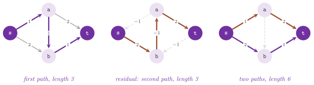
This residual digraph has negative lengths, but with the potentials \(\pi\) kept by the algorithm the reduced lengths (10.3) of its arcs are nonnegative, and each path can therefore be found by Dijkstra's algorithm, stopped when \(t\) reaches the top of the heap. Let \(\delta_\pi(v)\) be the reduced distance from \(s\) in \(G_x\) found by a search, \(\delta_\pi(t)\) that of \(t\), and \(P\) the path found. After the search, the potential of each node processed by it (i.e., removed from the heap before \(t\)) is increased by \(\delta_\pi(v)-\delta_\pi(t)\), and the others are left as they are.
Algorithm 10.5 (Successive shortest paths with
potentials, Suurballe::findFlow( t , k ) after init( s )).
1  x := 0; pi := 0; i := 0
2  while i < k:
3     run Dijkstra from s on the residual digraph (10.8) with the reduced lengths (10.3),
      stopping when t is on the top of the heap
4     if t is not reached: stop
5     for each node v processed: pi(v) := pi(v) + dist(v) - dist(t)
6     push one unit along the path found: x := 1 on its forward arcs, 0 on the reversed ones
7     i := i + 1
8  return i
Lemma 10.2. Suppose that the reduced lengths of all the arcs of \(G_x\) are nonnegative before an iteration of Algorithm 10.5 that finds a path \(P\). Then, after it, the reduced lengths of all the arcs of the new residual digraph are nonnegative, and those of the arcs of \(P\) (and of their reverses) are zero.
Proof. Let \(\eta(v)=\min\{\delta_\pi(v),\delta_\pi(t)\}\). The update of step 5 is \(\pi'(v)=\pi(v)+\eta(v)-\delta_\pi(t)\) for every node \(v\): a processed node has \(\delta_\pi(v)\le\delta_\pi(t)\), and a node not processed has \(\delta_\pi(v)\ge\delta_\pi(t)\) (possibly \(+\infty\)), by Theorem 10.2. For an arc \(uv\) of \(G_x\), one has \(\delta_\pi(v)\le\delta_\pi(u)+\ell_\pi(uv)\) by (10.2) for the distances, and therefore \(\eta(v)\le\eta(u)+\ell_\pi(uv)\), since \(\ell_\pi(uv)\ge 0\); hence, \(\ell_{\pi'}(uv)=\ell_\pi(uv)+\pi'(u)-\pi(u)-\pi'(v)+\pi(v)\ge 0\). Along \(P\), whose nodes before \(t\) are processed and on which \(\delta_\pi\) grows exactly by the reduced lengths, the same inequality is an equality, and \(\ell_{\pi'}=0\). The new residual digraph has the arcs of \(G_x\) not on \(P\) and the reverses of the arcs of \(P\), whose reduced lengths are the opposite of zero. \(\square\)
Theorem 10.6. After \(i\) iterations, \(x\) is an optimal solution of (10.7) with \(k=i\), and
If the loop stops at step 4, there are no \(i+1\) arc-disjoint paths from \(s\) to \(t\). The algorithm takes \(O(k\,(n+m)\log n)\) time with the binary heap.
Proof. Conditions (10.9) say that the reduced lengths of the arcs of \(G_x\) are nonnegative, the arc \(vu\) of an arc \(uv\) with \(x_{uv}=1\) having reduced length \(-\ell_\pi(uv)\). They hold at the start, with \(x=0\), \(\pi=0\) and \(\ell\ge 0\), and are kept by Lemma 10.2. The flow \(x\) satisfies the constraints of (10.7) with \(k=i\), since each iteration sends one unit along a path from \(s\) to \(t\) of \(G_x\). For any other feasible \(x'\), summing (10.3) gives \(\sum_a\ell(a)x'_a=\sum_a\ell_\pi(a)x'_a+i\,(\pi(t)-\pi(s))\), and the same for \(x\). Hence, \(\ell(x')-\ell(x)=\sum_a\ell_\pi(a)(x'_a-x_a)\ge 0\), since each term is nonnegative by (10.9) (where \(x_a=0\), \(x'_a-x_a\ge 0\); where \(x_a=1\), \(x'_a-x_a\le 0\)). If the loop stops at step 4, let \(X\) be the set of the nodes reachable from \(s\) in \(G_x\). Then \(t\notin X\), and each arc out of \(X\) has \(x=1\) and each arc into \(X\) has \(x=0\), otherwise \(G_x\) would leave \(X\). Hence, the arcs out of \(X\) are exactly \(i\) by the constraints of (10.7), and \(i+1\) arc-disjoint paths, each of which leaves \(X\), cannot exist. Each iteration is one search of Dijkstra plus \(O(n+m)\) work. \(\square\)
The first search runs on the lengths, since all the potentials are zero, and
the potentials of the nodes that it does not process stay zero. Then the paths
are extracted from \(x\) by findPaths(), which follows from \(s\) the arcs of
unit flow not yet used, scanning the arcs out of the current node from the
first one. By the constraints of (10.7), it can always leave a node other than
\(t\), and since each step uses up an arc it reaches \(t\). It takes \(O(km)\) time
when \(x\) has no cycle (a path then visits no node twice), and \(O(m\Delta)\) in
general, where \(\Delta\) is the largest out-degree, since it makes at most \(m\)
steps. Also, the node-disjoint version of the problem is solved by the same
class on the digraph of the adaptor SplitNodes of chapter
5, in which each node is split into an arc of capacity
one.
Interface. Suurballe< GR , LEN , TR > takes the digraph type, the type
of the length map (by default GR::ArcMap< int >) and the traits class, by
default SuurballeDefaultTraits< GR , LEN >. These traits give Digraph,
LengthMap, Length (the type of the lengths), FlowMap (an
ArcMap< int >), PotentialMap (a NodeMap of the lengths), Path (a
lemon::Path, or any path type with addBack()), and the HeapCrossRef and
the Heap (a BinHeap) of the internal searches; the named parameters
SetFlowMap< T >, SetPotentialMap< T >, SetPath< T > and
SetHeap< H , CR > change them. Its constructor takes the digraph and the
lengths, which must be nonnegative. The setters flowMap( m ) and
potentialMap( m ) set the maps of the flow and of the potentials (allocated
otherwise), and the searches are made by its private class ResidualDijkstra.
A call run( s , t , k ) is init( s ) followed by start( t , k ), with
\(k=2\) by default, and returns the number of paths found, i.e., \(k\) if there
are at least \(k\) arc-disjoint paths, and their largest number otherwise. In
turn, start( t , k ) is findFlow( t , k ) (Algorithm 10.5) followed by
findPaths(). If the paths from one source to many targets are needed,
fullInit( s ) replaces init( s ). It runs one complete search of Dijkstra
from s on the lengths, which then serves as the first iteration of each
subsequent start( t , k ), with \(\pi\) equal to the distances from \(s\) (for
which Lemma 10.2 holds as well, since they satisfy (10.2) and are tight on the
tree of the search). Each such call thus runs only \(k-1\) searches, and returns
0 when t cannot be reached from s, as it does after init( s ).
abLEMON
In LEMON 1.3.1, after fullInit( s ), findFlow( t , k ) took the first
path from the complete search without checking that t was reached,
counted one path for a target that cannot be reached, and findPaths()
then did not end; the test suurballe_test checks such a target.
Its queries are totalLength() (the length of the flow, computed in \(O(m)\)),
flow( a ) and flowMap(), potential( v ) and potentialMap() (an optimal
dual solution, i.e., potentials that satisfy (10.9) with the flow),
pathNum() and path( i ) for \(i\) from 0 to pathNum() \(-1\).
The program manual/examples/10-suurballe.cc (the test
manual_10_suurballe) solves the instance of Figure 10.1, checks that the two
paths are arc-disjoint and that the flow and the potentials satisfy (10.9),
and looks for a third path, which does not exist.
10.6 Exercises¶
Exercise 10.1. Show by an example that
Dijkstra's algorithm may give a wrong distance when one arc has a negative
length, although no cycle is negative, point out the step of the proof of
Theorem 10.2 that fails, and check the example against BellmanFord. (The
test test/dijkstra_test.cc exercises the interface of Dijkstra.)
Exercise 10.2. Compute the paths of least
bottleneck of a digraph with the operation traits of the program
manual/examples/10-dijkstra.cc, and verify that they satisfy the two
hypotheses of Theorem 10.2; then show that the product of the lengths, with
lengths in \((0,1]\) and the comparison reversed, also does, and gives the paths
of greatest reliability.
Exercise 10.3. Compare the number of nodes
scanned by Dijkstra::run( s , t ), by BidirDijkstra and by AStar with
the Manhattan distance on a grid of \(100\times 100\) nodes with random lengths
at least 1, for random pairs of nodes. (The test test/point_to_point_test.cc
checks the two point-to-point classes against Dijkstra, with heuristics that
are zero, exact, half the exact one, and admissible but not consistent.)
Exercise 10.4. Find a negative cycle anywhere in
a digraph by init( 0 ) and checkedStart() of BellmanFord, and explain
why init( 0 ) is equivalent to adding a new source joined to each node by an
arc of length zero. (The program manual/examples/10-bellman-ford.cc and the
test test/bellman_ford_test.cc find negative cycles.)
Exercise 10.5. Use Suurballe on the digraph of
SplitNodes to find two node-disjoint paths of least total length, and verify
that they share no inner node. (The test test/suurballe_test.cc checks the
flow, the potentials and the paths.)
Exercise 10.6. Show that, after \(i\) paths, the
value \(\pi(t)-\pi(s)\) of the potentials of Algorithm 10.5 is the length, in
the residual digraph (10.8) of the previous flow, of the last path found, and
check it by running the program manual/examples/10-suurballe.cc with \(k=1\)
and \(k=2\).