17. Matchings
We are concerned in this chapter with finding, in an undirected graph
\(G=(V,E)\) with \(n\) nodes and \(m\) edges, a set of edges no two of which share
an end, i.e., a matching, which is as large as possible, or of largest total
weight, or of least total cost among those that cover a prescribed set of
nodes. abLEMON solves these problems with three headers. The first,
bipartite_matching.h, holds the algorithms for bipartite graphs
(HopcroftKarp and MinCostAssignment). The second, matching.h, holds the
blossom algorithms of Edmonds for general graphs (MaxMatching,
MaxWeightedMatching and MaxWeightedPerfectMatching). The third,
fractional_matching.h, holds the algorithms for the relaxation in which an
edge may be taken by halves (MaxFractionalMatching,
MaxWeightedFractionalMatching and MaxWeightedPerfectFractionalMatching),
which matching.h also uses to start its weighted algorithms. Each class
gives, besides the matching, a dual solution that proves it optimal, and we
describe the two together, since one usually checks a result against its dual
(a "proof" that the user can verify in linear time, or nearly so). The
structure of the chapter is as follows. Section 17.1 states the problems and
the duality results on which the algorithms rest; sections 17.2 and 17.3 treat
the bipartite case, sections 17.4 and 17.5 the general one, section 17.6 the
fractional relaxations, and section 17.7 gives the exercises.
17.1 Problems, duality and the choice of an algorithm
Let \(\delta(u)\) denote the set of the edges incident to the node \(u\), \(\gamma(X)\) the set of the edges with both ends in \(X\subseteq V\), and \(N(X)\) the set of the nodes adjacent to at least one node of \(X\). A matching \(M\) covers the ends of its edges, and it is perfect when it covers all the nodes. The cardinality of a maximum matching is denoted by \(\nu(G)\). With a weight \(w_e\) on each edge, the maximum weight matching problem is the integer program
of which the maximum cardinality matching problem is the case \(w\equiv 1\) and the maximum weight perfect matching problem the case with equations in place of the inequalities (a minimum cost perfect matching is then found by negating the costs). The classes of this chapter ignore the loops, except where a flag of the fractional classes says otherwise (cf. section 17.6). An alternating path with respect to \(M\) is a path whose edges alternate between \(M\) and \(E\setminus M\). It is augmenting when it has at least one edge and neither of its ends is covered by \(M\). Exchanging the edges of \(M\) and of the path along an augmenting path \(P\) gives the matching \(M\oplus P\) (where \(\oplus\) is the symmetric difference) with one more edge, and the algorithms of the chapter that compute an integer matching all rest on the converse.
Theorem 17.1 (Berge). A matching \(M\) of \(G\) is maximum if and only if no path is augmenting with respect to \(M\).
Proof. If \(P\) is augmenting, \(M\oplus P\) is a larger matching. Conversely, let \(M^*\) be a matching with \(|M^*|>|M|\). Each node has at most one edge of \(M\) and one of \(M^*\) in \(M\oplus M^*\); hence, the subgraph \((V,M\oplus M^*)\) is made of node-disjoint paths and cycles whose edges alternate between the two matchings. A cycle has as many edges of \(M\) as of \(M^*\), and so has a path with an even number of edges; since \(|M^*\setminus M|>|M\setminus M^*|\), some path has one more edge of \(M^*\) than of \(M\), i.e., it starts and ends with an edge of \(M^*\). Its ends are not covered by \(M\) (an edge of \(M\) at an end would continue the path), and therefore the path is augmenting with respect to \(M\). \(\square\)
The result is due to Berge 1957
(cf. also Schrijver 2003, ch.
24). In a bipartite graph,
whose nodes are split into the red nodes \(R\) and the blue nodes \(B\) with
each edge joining a red node to a blue one (the BpGraph structures of
chapter 4), the dual object of a matching is a vertex
cover, i.e., a set of nodes that contains at least one end of each edge. In a
general graph the dual object is rather a set of nodes \(A\), called a
barrier, whose removal leaves many components with an odd number of nodes.
We denote by \(o(G-A)\) the number of the odd components of \(G-A\). The two weak
duality bounds are the following.
Lemma 17.1. (i) For a matching \(M\) and a vertex cover \(C\) of any graph, \(|M|\le|C|\). (ii) For a matching \(M\) and a set \(A\subseteq V\), at least \(o(G-A)-|A|\) nodes are left uncovered by \(M\); hence,
Proof. (i) Each edge of \(M\) has an end in \(C\), and distinct edges of \(M\) have distinct ends. (ii) In an odd component \(K\) of \(G-A\) the edges of \(M\) with both ends in \(K\) cover an even number of its nodes; hence, at least one node of \(K\) is either uncovered or matched to a node of \(A\). At most \(|A|\) components are of the second kind, and therefore at least \(o(G-A)-|A|\) nodes are uncovered, i.e., \(2|M|\le n-o(G-A)+|A|\). \(\square\)
In a bipartite graph the first bound is tight. We give the proof here, since
HopcroftKarp computes the cover by its construction (cf. section 17.2).
Theorem 17.2 (König). In a bipartite graph the maximum cardinality of a matching equals the minimum cardinality of a vertex cover. More precisely, if \(M\) is a maximum matching and \(Z\) is the set of the nodes reachable from the uncovered red nodes by alternating paths that start with an edge not in \(M\), then \(C=(R\setminus Z)\cup(B\cap Z)\) is a vertex cover with \(|C|=|M|\).
Proof. Let \(rb\) be an edge with \(r\in R\) and \(b\in B\), and suppose that \(r\in Z\) and \(b\notin Z\). If \(rb\notin M\), the alternating path that reaches \(r\) ends at \(r\) with an edge of \(M\) or is empty (\(r\) uncovered), and it continues along \(rb\) to \(b\), against \(b\notin Z\). If \(rb\in M\), then \(r\) is covered, hence not a start, and it is reached only through its matching edge, i.e., from \(b\), again against \(b\notin Z\). Thus, each edge has its red end in \(R\setminus Z\) or its blue end in \(B\cap Z\), and \(C\) is a cover. Each blue node of \(Z\) is covered by \(M\) (otherwise the path that reaches it would be augmenting, against Theorem 17.1), and each red node outside \(Z\) is covered (the uncovered red nodes are in \(Z\)); furthermore, no edge of \(M\) has both ends in \(C\), since the mate of a blue node of \(Z\) is in \(Z\). Hence \(|C|\le|M|\), and equality follows from Lemma 17.1. \(\square\)
The result is due to König 1931 (cf. also Schrijver 2003, ch. 16). In a general graph a minimum vertex cover may be twice as large as a maximum matching (as in a triangle), and it is (17.2) that becomes tight.
Theorem 17.3 (Tutte–Berge formula). For every graph,
Proof. The inequality \(\le\) is (17.2). For the converse, Theorem 17.10 of
section 17.4 shows that, at the end of MaxMatching on \(G\), the set \(A\) of
the nodes with status ODD satisfies (17.2) with equality for the matching
found. \(\square\)
The formula is due to Tutte
1947 and Berge. The barrier
that MaxMatching returns is moreover the canonical one of the following
structure theorem, which we do not prove (its proof takes several pages).
Theorem 17.4 (Gallai–Edmonds decomposition). Let \(D\) be the set of the nodes left uncovered by at least one maximum matching, \(A\) the set of the nodes not in \(D\) with a neighbour in \(D\), and \(C=V\setminus(D\cup A)\). Then \(A\) attains the minimum in (17.3). Each component of the subgraph induced by \(D\) is factor-critical (i.e., it has a perfect matching after the removal of any one of its nodes). The subgraph induced by \(C\) has a perfect matching, and each maximum matching matches the nodes of \(A\) to nodes of \(D\) in distinct components.
Proof (sketch). One runs Edmonds' search of section 17.4 to its end and
shows that the nodes left EVEN are those of \(D\) (a node is EVEN exactly
when an alternating path of even length joins it to an uncovered root, and
exchanging along that path gives a maximum matching that leaves it uncovered),
that the ODD nodes are its neighbours, and that the blossoms of the EVEN
nodes are factor-critical. The full proof is in Schrijver 2003, ch.
24, after Gallai
1964 and Edmonds
1965a. \(\square\)
For the weighted problems the inequalities of (17.1) do not describe the convex hull of the matchings, since the point with \(x_e=\frac12\) on the edges of a triangle satisfies them and is not a combination of matchings. Let \(\mathcal O\) be the family of the subsets of \(V\) of odd cardinality at least 3; Edmonds showed that the odd set inequalities
are the missing ones, and the weighted classes of matching.h work on his
description. Its linear programming dual has a variable \(y_u\) for each node
and a variable \(z_S\ge 0\) for each odd set:
with \(y\ge 0\) for the version with inequalities and \(y\) free for the perfect version. The slack of the edge \(uv\) is \(y_u+y_v+\sum_{S:\,uv\in\gamma(S)}z_S-w_{uv}\), and the edge is tight when its slack is 0.
Lemma 17.2. Let \(M\) be a matching (a perfect one, in the perfect version) and \((y,z)\) a feasible solution of (17.5) such that (i) each edge of \(M\) is tight, (ii) each node with \(y_u>0\) is covered by \(M\) (in the version with inequalities), and (iii) each set \(S\) with \(z_S>0\) contains \(\frac{|S|-1}2\) edges of \(M\). Then \(M\) is a maximum weight matching (perfect matching), and \((y,z)\) is an optimal solution of (17.5).
Proof. Summing the equations (i) over the edges of \(M\) gives \(w(M)=\sum_{uv\in M}(y_u+y_v)+\sum_S z_S|M\cap\gamma(S)|\), which by (ii) and (iii) is the objective of (17.5). For any matching \(M'\) (perfect, in that version), the constraints of (17.5), \(y\ge 0\) (or \(M'\) perfect) and \(|M'\cap\gamma(S)|\le\frac{|S|-1}2\) give
The same chain applied to a feasible point of the relaxation proves the optimality of \((y,z)\). \(\square\)
Theorem 17.5 (Edmonds). The convex hull of the incidence vectors of the matchings of \(G\) is the set \(Q\) of the \(x\ge 0\) that satisfy \(\sum_{e\in\delta(u)}x_e\le 1\) for each \(u\in V\) and (17.4); that of the perfect matchings is obtained by turning the node inequalities into equations.
Proof. Let \(P\) be the convex hull; clearly \(P\subseteq Q\), and \(Q\) is a
polytope. For any \(w\), the algorithm of section 17.5 finds a matching \(M\) and
a feasible \((y,z)\) that satisfy the conditions of Lemma 17.2 (Theorem 17.12);
since the dual objective bounds \(w^\top x\) from above on \(Q\) (the chain of the
proof of Lemma 17.2), \(\max_P w^\top x\ge w(M)\ge\max_Q w^\top x\). Two
polytopes with the same maximum of each linear function coincide. The perfect
version is identical, with Theorem 17.12 for MaxWeightedPerfectMatching.
\(\square\)
The theorem is in Edmonds 1965b; cf. also Schrijver 2003, ch. 25 and 26. Dropping (17.4) gives the fractional matching problem, whose dual is (17.5) without the \(z\) variables. Its optimum bounds that of (17.1) from above, and a triangle with unit weights shows that the bound may be strict (\(\frac32\) against 1). The algorithms of section 17.6 always return an optimal fractional matching made of a matching, with value 1 on its edges, and of node-disjoint odd cycles, with value \(\frac12\) on theirs (Theorems 17.14 and 17.16). Indeed, each vertex of the fractional matching polytope has this form (Schrijver 2003, ch. 30).
As for the choice among the classes, a bipartite graph is best handled by
bipartite_matching.h, i.e., by HopcroftKarp for the cardinality, in
\(O((n+m)\sqrt n)\) time, and by MinCostAssignment for a matching of least
cost that covers all the red nodes, in \(O(n_R\,(n+m\log m))\) time with
\(n_R=|R|\). A general graph needs the blossoms (which make the algorithms
somewhat more involved), i.e., MaxMatching for the cardinality and
MaxWeightedMatching or MaxWeightedPerfectMatching for the weights, the
latter two in \(O(nm\log n)\) time. In our view, the fractional classes are
mostly of interest when the relaxation is itself the object (e.g., as a
bound), and as the starting point of the weighted blossom algorithms, which
call them by default. Of course, one can also write an assignment problem as a
minimum cost flow problem (chapter 13), and a
bipartite cardinality matching as a maximum flow problem (chapter
12). This requires building the network, which may be
rather wasteful when the graph is "large". The classes of this chapter work on
the graph itself, and they give the dual objects described above directly.
17.2 Maximum cardinality matching in bipartite graphs
HopcroftKarp< BPGR > finds a maximum matching of a bipartite graph of type
BPGR, together with the minimum vertex cover of Theorem 17.2, by the
algorithm of Hopcroft and Karp
1973. The algorithm grows the
matching in phases. In each phase a breadth-first search from the uncovered
red nodes labels each red node \(r\) with the number \(d(r)\) of matched edges on
a shortest alternating path that reaches it from an uncovered red node, and it
stops at the first layer \(L\) from which an uncovered blue node is adjacent. An
augmenting path then has \(2L+1\) edges at least. Then a depth-first search from
each uncovered red node follows these labels, one layer at a time, until it
meets an uncovered blue node from layer \(L\), and the matching is augmented
along the path found.
Algorithm 17.1 (Hopcroft–Karp).
 1  M <- greedy matching (greedyInit) or empty matching (init)
 2  loop
 3     for each red r do d(r) <- 0 if r is uncovered, d(r) <- inf otherwise
 4     breadth-first search from the uncovered red nodes: take x from the
        queue; if d(x) >= L then stop; for each edge xb, if b is uncovered
        then L <- d(x), else, if b is matched to y and d(y) = inf, then
        d(y) <- d(x) + 1 and y enters the queue (L = inf at the start)
 5     if L = inf then exit the loop
 6     for each red node s, in the order of RedNodeIt, if s is uncovered do
 7        depth-first search from s: at a red x, scan the edges xb from the
           one x stopped at; if b is uncovered and d(x) = L, augment M along
           the path found and stop; if b is matched to y with
           d(y) = d(x)+1 <= L, go down to y
 8        a red node all of whose remaining edges fail gets d <- inf, and
           its parent moves to its next edge
 9  Z <- nodes reached by alternating paths from the uncovered red nodes
10  cover <- (red nodes not in Z) + (blue nodes in Z)
Steps 3 to 5 are bfs(), steps 7 and 8 dfs(), and steps 9 and 10
findCover(), which is called once at the end of start(). The depth-first
search is written without recursion, and each red node keeps in the map
_current the edge it has reached, which is reset only at the start of a
phase. The certificate does not depend on the phases, since step 10 builds it
from the final matching alone, as in the proof of Theorem 17.2. The bound of
the method rests on the following property of shortest augmenting paths, in
which \(|P|\) is the number of edges of a path \(P\).
Lemma 17.3. (i) Let \(P\) be a shortest augmenting path with respect to a matching \(M\) of any graph, and \(P'\) an augmenting path with respect to \(M\oplus P\). Then \(|P'|\ge|P|+2|P\cap P'|\), where \(P\cap P'\) is the set of their common edges. (ii) Let \(M_0\) be a matching, and \(P_1,\dots,P_k\) paths such that each \(P_i\) is a shortest augmenting path with respect to \(M_{i-1}\), where \(M_i=M_{i-1}\oplus P_i\). Then \(|P_1|\le\dots\le|P_k|\), and two of the paths with the same number of edges are node-disjoint.
Proof. (i) The matching \(N=M\oplus P\oplus P'\) has \(|M|+2\) edges, and \(M\oplus N=P\oplus P'\). As in the proof of Theorem 17.1, \(M\oplus N\) contains at least two node-disjoint paths augmenting with respect to \(M\), each with at least \(|P|\) edges; hence \(|P|+|P'|-2|P\cap P'|=|P\oplus P'|\ge 2|P|\). (ii) The monotonicity follows from (i). Let \(i<j\) be such that \(|P_i|=|P_j|\) and \(P_i\), \(P_j\) share a node, with \(j-i\) least. Then \(P_j\) is node-disjoint from \(P_{i+1},\dots,P_{j-1}\) (their lengths are between the two), and therefore it is augmenting with respect to \(M_i\) as it is with respect to \(M_{j-1}\). By (i), \(P_i\) and \(P_j\) share no edge. However, a common node \(v\) is covered in \(M_i\) by an edge of \(P_i\), and it is an inner node of \(P_j\), which then contains that edge, a contradiction. \(\square\)
Lemma 17.4. In a phase with \(L<\infty\), each path along which step 7 augments has \(2L+1\) edges and is a shortest augmenting path with respect to the current matching, and these paths are node-disjoint. At the end of the phase, any augmenting path has more than \(2L+1\) edges.
Proof. Step 4 is a breadth-first search on the red nodes, in which a red node \(y\) is reached from \(x\) through a non-matching edge \(xb\) and the matching edge \(by\); hence, for each red node \(r\) with \(d(r)\le L\), \(d(r)\) is the number of matched edges of a shortest alternating path from an uncovered red node to \(r\), and \(2L+1\) is the length of a shortest augmenting path at the start of the phase. A path found by step 7 visits red nodes with \(d=0,1,\dots,L\) and ends with an edge to an uncovered blue node; hence, it has \(2L+1\) edges, and, by Lemma 17.3(ii) and by induction on the paths of the phase, it is a shortest augmenting path for the matching it augments, and it is node-disjoint from the previous ones. Suppose now that, at the end of the phase, \(Q\) is an augmenting path with \(2L+1\) edges, with red nodes \(r_0,\dots,r_L\) (in this order, \(r_0\) uncovered) and blue nodes \(b_0,\dots,b_L\) (\(b_L\) uncovered). By Lemma 17.3(ii), applied to the paths of the phase followed by \(Q\), no node of \(Q\) is on a path of the phase; hence, \(Q\) was augmenting at the start of the phase, with the same matching edges \(b_jr_{j+1}\) throughout. The search of step 4 gives \(d(r_0)=0\) and \(d(r_{j+1})\le d(r_j)+1\), and \(d(r_L)\ge L\), since the tree path to \(r_L\) followed by \(r_Lb_L\) is augmenting; hence \(d(r_j)=j\) for each \(j\). Furthermore, the pointer of \(r_L\) never passes the edge \(r_Lb_L\), which is accepted whenever it is scanned, and, by backward induction, the pointer of \(r_j\) never passes \(r_jb_j\), which it leaves only when \(r_{j+1}\) fails. Thus no \(r_j\) fails. Then the search of step 7 from \(r_0\), which is uncovered when its turn comes, either augments, covering \(r_0\), or fails, and both contradict what we have shown. \(\square\)
Theorem 17.6. After start(), the matching is
maximum, and cover() describes a vertex cover with matchingSize() nodes,
i.e., a minimum one.
Proof. The loop ends when step 4 meets no uncovered blue node, i.e., when no alternating path from an uncovered red node reaches an uncovered blue node. Every augmenting path of a bipartite graph has an uncovered red end, and therefore the matching is maximum by Theorem 17.1. The cover is the set \(C\) of Theorem 17.2. \(\square\)
Theorem 17.7. start() performs at most
\(2\sqrt n+2\) phases and runs in \(O((n+m)\sqrt n)\) time; greedyInit() and
init() run in \(O(n+m)\) time.
Proof. A phase costs \(O(n+m)\). The breadth-first search scans each edge
once. In the depth-first searches a red node is pushed on the stack only along
the edge its parent points to, and that pointer moves forward when the node
fails. It stays only along a path just augmented, and those paths are
node-disjoint (Lemma 17.4), and therefore each pointer moves at most once per
edge and the augmentations cost \(O(n)\) in total. Also findCover() is a
breadth-first search. By Lemma 17.4, after \(k\) phases each augmenting path has
at least \(2k+1\) edges, i.e., \(2k+2\) nodes. Let \(M\) be the matching after
\(k=\lceil\sqrt n\,\rceil\) phases and \(M^*\) a maximum one: as in the proof of
Theorem 17.1, \(M\oplus M^*\) contains \(|M^*|-|M|\) node-disjoint augmenting
paths, each with more than \(2\sqrt n\) nodes, and therefore
\(|M^*|-|M|<\sqrt n/2\). Each further phase but the last augments at least once,
and the number of phases is at most
\(\lceil\sqrt n\,\rceil+\sqrt n/2+1\le 2\sqrt n+2\). \(\square\)
The class states this bound, and the bound \(O(m\sqrt n)\) on a graph without
isolated nodes. The bound is usually far from attained in practice. This class
follows the pattern of the algorithm classes of chapter
3, although it has no named template parameters,
since it uses no auxiliary structure that one could replace. Its types are
BpGraph (i.e., BPGR) and MatchingMap, i.e., BpGraph::NodeMap< Edge >,
and its constructor HopcroftKarp( const BpGraph & graph ) builds the maps of
the matching, of the layers and of the cover. Execution starts with init(),
which empties the matching, or with greedyInit(), which also matches each
red node, in the order of RedNodeIt, to the first uncovered blue node among
its neighbours (in the order of IncEdgeIt). Then start() augments the
matching until it is maximum and computes the cover, and run() is simply
greedyInit() followed by start(). Among the queries, matchingSize(),
matching( const Edge & ) (whether the edge is in the matching),
matching( const Node & ) (the matching edge at the node, or INVALID),
matchingMap() (a const reference to the map of the matching) and
mate( const Node & ) give the primal solution. Finally,
cover( const Node & ) returns whether the node is in the minimum vertex
cover. It is meaningful only after start() or run(), and before them it is
false on every node.
abLEMON
Both HopcroftKarp and MinCostAssignment are new in abLEMON (version
1.5.0, LEMON trac ticket #168). LEMON 1.3.1 has bipartite graphs but no
matching algorithm written for them. Its general matching classes give no
vertex cover and no assignment potentials.
17.3 Minimum cost assignment
We now give a cost \(c_e\) to each edge of a bipartite graph, which may have any
number of blue nodes and need not be complete. In this setting
MinCostAssignment< BPGR , CM > solves
i.e., it finds a matching of least cost among those that cover all the red nodes, if one exists. Its dual solution is a potential \(\pi\) on the nodes with
with equality on the edges of the matching, and with the blue nodes left uncovered all at the largest potential \(K=\max_{b\in B}\pi(b)\) of the blue nodes; \(\bar c_e\) is the reduced cost of \(e\). Setting \(\alpha_r=K-\pi(r)\) and \(\beta_b=\pi(b)-K\le 0\) gives a feasible solution of the linear programming dual of the relaxation of (17.6), i.e., \(\max\{\sum_r\alpha_r+\sum_b\beta_b:\alpha_r+\beta_b\le c_{rb},\beta\le0\}\), whose value equals the cost of the matching (each matched blue node \(b_r\) contributes \(\pi(b_r)-K\), each uncovered one 0). Thus, the optimal cost is \(\sum_{r\in R}\big(\pi(b_r)-\pi(r)\big)\), where \(b_r\) is the mate of \(r\).
The method is that of the successive shortest augmenting paths, with the potentials of Edmonds and Karp 1972 and Tomizawa 1971. Here the red nodes are matched one at a time, each along a shortest path of the residual graph, in which an edge not in the matching is traversed from its red end to its blue end at cost \(c_e\) and an edge of the matching from its blue end to its red end at cost \(-c_e\). The reduced cost of the second traversal is \(-\bar c_e\). Each path is found by Dijkstra's algorithm (Dijkstra 1959) on the reduced costs, which (17.7) keeps nonnegative.
Algorithm 17.2 (Successive shortest paths for the assignment).
 1  M <- empty; pi(v) <- 0 for each node v
 2  for each red r do if r has no edge then return false, else
       pi(r) <- - (least cost of an edge of r)
 3  for each red node s, in the order of RedNodeIt do
 4     Dijkstra from s, d(s) = 0, on the reduced costs: red x -> blue b
        along xb not in M at d(x) + c(xb) + pi(x) - pi(b); matched blue b
        -> its mate y at d(b) - (c(yb) + pi(y) - pi(b)); stop when an
        uncovered blue node t is taken from the heap
 5     if no uncovered blue node is taken then return false
 6     for each node v do pi(v) += d(v) if v was taken from the heap with
        d(v) < d(t), and pi(v) += d(t) otherwise
 7     augment M along the path from s to t
 8  return true
Step 4 and the rest of each iteration are the private function augment().
The heap of step 4 is a std::priority_queue of pairs (distance, node id)
with lazy deletion: a node reached again at a shorter distance is pushed
again, and the stale entries are skipped when popped. The correctness rests on
the following invariant.
Lemma 17.5. Before each search of step 4, (17.7) holds, the edges of \(M\) have zero reduced cost, and all the uncovered blue nodes have the same potential, the largest of the blue nodes.
Proof. After step 2, \(\bar c_{rb}=c_{rb}-\min_{e\in\delta(r)}c_e\ge 0\), \(M\) is empty and all the blue potentials are 0. Assume the claim before a search, let \(d(v)\) be the distance from \(s\) in the residual graph with the reduced costs (which are nonnegative, and therefore the distances of the nodes taken from the heap are exact), with \(d(v)=\infty\) for the nodes not reached, and let \(\pi'=\pi+\min\{d,d(t)\}\), which is the update of step 6 (a node not taken has \(d\ge d(t)\)). For a residual arc from \(x\) to \(y\) with reduced cost \(\bar c\ge0\), the new reduced cost is \(\bar c+\min\{d(x),d(t)\}-\min\{d(y),d(t)\}\), which is nonnegative since \(d(y)\le d(x)+\bar c\). On the path from \(s\) to \(t\), whose nodes have \(d\le d(t)\) and satisfy \(d(y)=d(x)+\bar c\), the new reduced costs are zero, and the augmentation of step 7 reverses only arcs of zero reduced cost; hence, (17.7) holds after the iteration, with equality on \(M\). The search stops at the first uncovered blue node taken from the heap; hence, each other uncovered blue node gets the increase \(d(t)\), which no other blue node exceeds, and \(t\) becomes covered. \(\square\)
Theorem 17.8. run() returns true if and
only if a matching that covers all the red nodes exists. In that case the
matching is an optimal solution of (17.6), and potential() gives the dual
solution (17.7).
Proof. A red node without edges cannot be covered. If the search from \(s\) meets no uncovered blue node, let \(X\) be the set of the nodes it reaches: every blue node of \(X\) is matched to a red node of \(X\) (the only residual arc out of a matched blue node goes to its mate), each blue neighbour of a red node of \(X\) is in \(X\), and \(s\) is the only uncovered red node of \(X\); hence, the \(|X\cap B|+1\) red nodes of \(X\) have only \(|X\cap B|\) blue neighbours, and no matching covers them. Otherwise each iteration covers one more red node and keeps the others covered, and at the end Lemma 17.5 and the computation after (17.7) give a feasible dual solution of the relaxation with the value of the matching, which is therefore optimal. \(\square\)
Theorem 17.9. run() takes
\(O(n_R\,(n+m\log m))\) time, i.e., \(O(n_R\,(n+m\log n))\) on a graph without
parallel edges.
Proof. Step 2 takes \(O(n+m)\) time. In a search each red node taken from the heap relaxes its edges once and each blue node one edge; hence, at most \(m+n+1\) pairs enter the heap, each at a cost of \(O(\log m)\). Step 6 takes \(O(n)\) time, and step 7 and the reset of the marks take time proportional to the nodes reached. There are at most \(n_R\) searches. \(\square\)
The class states the same bound, in which the term \(n_R\,n\) of the updates of
step 6 matters only when \(m\) is smaller than \(n\), i.e., when many blue nodes
are isolated. Note that the comparisons are exact (the class has no
tolerance), which is usually adequate for integer costs but may be somewhat
fragile with floating-point ones, and that the cost type must be a signed
arithmetic type. The interface is reduced to what the method needs. Its types
are BpGraph, CostMap (i.e., CM, by default BpGraph::EdgeMap< int >),
Value (the type of the costs) and MatchingMap (as in HopcroftKarp), and
its constructor is MinCostAssignment( const BpGraph & graph , const CostMap &
cost ). Its only execution function is run(), which returns true if a
matching covering all the red nodes exists and false otherwise (in which
case the matching is left as the method had grown it, and the potentials have
no meaning). As in HopcroftKarp, totalCost(), matching( const Edge & ),
matching( const Node & ) and matchingMap() give the primal solution, while
potential( const Node & ) gives the dual solution (17.7).
The program manual/examples/17-bipartite.cc (the test manual_17_bipartite)
solves a "small" instance with both classes of the header: it checks the cover
of Theorem 17.2, the conditions (17.7) and the value of the dual solution, and
it compares the optimal cost with an enumeration of all the assignments.
17.4 Maximum cardinality matching in general graphs
We now turn to general graphs, in which an alternating search tree may close
an odd cycle, and the search then has to treat the cycle as a single node.
This is the blossom of Edmonds
1965a, and MaxMatching< GR >
implements his alternating forest algorithm on an undirected graph of type
GR. Each node has a status, EVEN, ODD, MATCHED or UNMATCHED. At the
start the covered nodes are MATCHED and the others UNMATCHED. A search
tree is grown from an UNMATCHED root, which becomes EVEN. A MATCHED node
reached from an EVEN node becomes ODD, and its mate EVEN. An edge
between two EVEN nodes of the same tree in distinct blossoms closes a
blossom, i.e., an odd cycle of blossoms of the tree, which is merged into one
blossom whose nodes are all EVEN. An edge from an EVEN node to an
UNMATCHED node gives an augmenting path. Internally, the blossoms are kept
by a UnionFindEnum and the trees by an ExtendFindEnum (see chapter
8), and each node of a blossom keeps an ear, i.e.,
the arc along which an even alternating path inside the blossom leaves it
towards the base of the blossom (the node through which the blossom is
attached to its parent in the tree).
Algorithm 17.3 (Edmonds' alternating forest, sparse variant).
 1  M <- empty, greedy or given matching; covered nodes MATCHED, the
       others UNMATCHED
 2  for each node r, in the order of NodeIt, while more than l nodes are
       UNMATCHED (l = 0, or l = 1 without the decomposition) do
 3     if r is UNMATCHED then r becomes the EVEN root of a new tree; Q <- (r)
 4     while Q is not empty do take u from Q; for each arc uv do
 5        if v is EVEN and in another blossom then shrink the blossom closed
           by uv; its ODD nodes become EVEN and enter Q
 6        if v is MATCHED then extend: v becomes ODD, its mate EVEN (into Q)
 7        if v is UNMATCHED then augment along uv and the tree path of u; the
           nodes of the tree become MATCHED; go to the next root
 8        (if v is ODD, or EVEN in the blossom of u, nothing happens)
 9  (a tree that did not augment keeps its statuses)
Step 5 is shrinkOnEdge(), step 6 extendOnArc() and step 7
augmentOnArc(), and the loop of steps 4 to 8 is processSparse(). A tree
that ends without augmenting is called Hungarian, and the analysis rests on
what it leaves behind.
Lemma 17.6. When the search from a root ends
without augmenting, every neighbour of an EVEN node of its tree is an ODD
node (of this or of an earlier tree) or an EVEN node of the same blossom.
The statuses of the nodes of a Hungarian tree do not change afterwards, and
each of its blossoms has an odd number of nodes and induces a connected
subgraph.
Proof. Each node that becomes EVEN enters the queue (as the root, as the
mate of a new ODD node, or by a shrink), and all its arcs are scanned. A
scanned arc to an EVEN node of another blossom is shrunk, to a MATCHED
node extends the tree, and to an UNMATCHED node augments, and one to an
ODD node is left alone. Hence, at the end of a search without augmentation,
an EVEN node has no MATCHED or UNMATCHED neighbour and no EVEN
neighbour in another blossom of its tree. It has none in an earlier Hungarian
tree either, since such a neighbour would have a neighbour outside its own
tree, against the claim for that tree. A later search reaches only MATCHED,
UNMATCHED and EVEN nodes of its own tree from its EVEN nodes, and the
nodes of a Hungarian tree are neither of these; hence, it never touches them.
Finally, a blossom is either a single node or the union of an odd number of
blossoms joined in a cycle by edges, each with an odd number of nodes, which
gives the parity and the connection. \(\square\)
Theorem 17.10. At the end of startSparse()
or startDense() the matching is maximum. With the decomposition, the set \(A\)
of the ODD nodes attains the minimum in (17.3), the subgraphs induced by the
blossoms of the EVEN nodes are the odd components of \(G-A\) that contain
them, and the MATCHED nodes are matched among themselves.
Proof. At the end, each uncovered node is the root of a Hungarian tree,
except at most one UNMATCHED node \(u\) that was never searched from (without
the decomposition). In a tree, each node but the root is covered, an ODD
node is matched to an EVEN node of the tree, and the number of the EVEN
blossoms exceeds by one the number of the ODD nodes (an extension adds one
of each, and a shrink of \(2k+1\) blossoms removes \(k\) ODD nodes and \(2k\)
EVEN blossoms). The mate of a MATCHED node is MATCHED. By Lemma 17.6, an
EVEN blossom has no neighbour outside \(A\), and therefore it is an odd
component of \(G-A\). Also \(u\), which has no EVEN neighbour by the same lemma,
lies in a component of \(G-A\) made of \(u\) and of MATCHED nodes matched among
themselves, i.e., in an odd one. If \(h\) is the number of the Hungarian trees,
the number of the uncovered nodes is \(h\) (or \(h+1\), counting \(u\)) and
\(o(G-A)\ge h+|A|\) (or \(h+1+|A|\)); hence \(n-2|M|\le o(G-A)-|A|\), and by Lemma
17.1 both the matching and \(A\) are optimal. \(\square\)
Hence, with the decomposition the statuses give the barrier that proves the
matching maximum by (17.3). By Theorem 17.4 and its proof they are, moreover,
the canonical decomposition, the EVEN nodes forming \(D\), the ODD nodes \(A\)
and the MATCHED nodes \(C\). Without the decomposition, the loop of step 2
stops when at most one node is left UNMATCHED, i.e., uncovered and never
searched from. The matching is still maximum, but \(u\) has no status of the
decomposition, and the statuses do not form it. According to the header, this
may save much time, in particular on a dense graph with an odd number of
nodes, where the last search, from a node that remains uncovered, usually
explores most of the graph and finds no augmenting path.
The variant startDense() runs the same search, in processDense(), with the
heuristic of postponing the shrinks. It first extends the tree from all the
nodes in the queue, augmenting as soon as it can. Only when no extension or
augmentation is left does it scan the arcs of the queued nodes again for the
shrinks, extending (and possibly augmenting) again from the nodes that each
shrink makes EVEN. The header reports this to be faster on "dense" graphs
(presumably a matter of constants, since the worst case is the same). Lemma
17.6 and Theorem 17.10 hold for it with the same proofs, since each EVEN
node still has all its arcs scanned for the three cases. The header states no
bound on the running time. The following one, for this implementation, is not
the best known for the problem, which is \(O(m\sqrt n)\) (Galil
1986 surveys the implementations of
the blossom algorithm).
Theorem 17.11. startSparse() and
startDense() run in \(O(n\,m\,\alpha(n)+n^3\log n)\) time, where \(\alpha\) is
the inverse of Ackermann's function.
Proof (sketch). There is at most one search per node. In a search, each node
becomes EVEN at most once and is queued once, and its arcs are scanned once
(twice in the dense variant), each scan costing a find() of the union-find
structure, i.e., \(O(\alpha(n))\) amortized (it joins by size and compresses the
paths). A search makes at most \(n/2\) extensions and at most \(n/2\) shrinks,
since a shrink merges at least three blossoms of the tree into one. A shrink
first finds the nearest common ancestor of the two blossoms by walking up from
both alternately and storing the visited bases in two std::sets, at a cost
of \(O(n\log n)\). Then it redirects the ears along the two paths, walking
inside each blossom of the paths from the node where the path enters it to its
base, which costs \(O(n)\) in total, since these walks visit distinct nodes. An
augmentation, and the reset of the statuses of the tree at its end, cost
\(O(n)\). Hence, a search costs \(O(m\,\alpha(n)+n^2\log n)\). \(\square\)
Besides the constructor MaxMatching( const Graph & graph ), the class has
three functions that set the initial matching. These are init() (the empty
one), greedyInit() (each node, in the order of NodeIt, matched to its
first uncovered neighbour in the order of OutArcIt, loops excluded) and
matchingInit( const MatchingMap & matching ), a template on the type of the
map, which takes a bool edge map and returns false if two edges with value
true share a node (in which case the matching is left half built, and the
function must be called again before a start). Two functions,
startSparse( bool decomposition = true ) and
startDense( bool decomposition = true ), run the two variants of Algorithm
17.3, after one of the three initializations, and
run( bool decomposition = true ) calls greedyInit() and startSparse() if
\(m<2n\), and init() and startDense() otherwise. The types of the class are
Graph (i.e., GR), MatchingMap (i.e., Graph::NodeMap< Arc >) and
StatusMap (i.e., Graph::NodeMap< Status >). Of the queries,
matchingSize() counts the covered nodes (in \(O(n)\) time), and
matching( const Edge & ), matching( const Node & ) (the matching arc at
the node, directed away from it, or INVALID), matchingMap() and
mate( const Node & ) complete the primal solution. Lastly,
status( const Node & ) and statusMap() give the values of the enum
Status, i.e., EVEN \(=1\) (also called D), MATCHED \(=0\) (also C),
ODD \(=-1\) (also A) and UNMATCHED \(=-2\), and barrier( const Node & ) is
true on the ODD nodes.
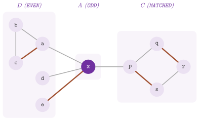
The program manual/examples/17-edmonds.cc (the test manual_17_edmonds)
computes the matching of Figure 17.1, counts the components of the subgraph
induced by the EVEN nodes with a FilterNodes adaptor (chapter
5) and countConnectedComponents() (chapter
18), checks the equality of (17.3) for the barrier
found, and runs the algorithm once more without the decomposition.
abLEMON
The parameter decomposition of startSparse(), startDense() and
run() is not in LEMON 1.3.1: it was added to the repository of LEMON in
2018, after its last release, and abLEMON is the first release to
distribute it. With the default true, a program written for LEMON 1.3.1
behaves as before.
17.5 Maximum weight matchings in general graphs
MaxWeightedMatching< GR , WM > solves (17.1), and
MaxWeightedPerfectMatching< GR , WM > its perfect version, by the
primal-dual blossom algorithm of Edmonds
1965a. Throughout, the algorithm
keeps a matching, a family of nested blossoms and a dual solution of (17.5)
with \(z_S>0\) only on blossoms, and it changes the duals until all the nodes
are covered or, in the version with inequalities, until the uncovered nodes
have \(y_u=0\). Its weight map WM defaults to GR::EdgeMap< int >, and loops
are ignored. Both classes use binary heaps (BinHeap) for the kinds of dual
change, four in MaxWeightedMatching and three in the perfect version, and a
HeapUnionFind for the nested blossoms, which gives the bound \(O(nm\log n)\)
stated by the header, i.e., that of Galil, Micali and Gabow
1986. In the following, a node or a
blossom is in the forest when it belongs to an alternating tree rooted at an
uncovered blossom, EVEN or ODD as in section 17.4. The others are
MATCHED, and they include the nodes that left the forest uncovered with
\(y_u=0\).
Algorithm 17.4 (Primal-dual blossom algorithm).
 1  init: y(u) <- max over the edges e at u of w(e)/2, and at least 0 in
       the version with inequalities; z <- 0; M empty; or fractionalInit:
       y and M from the optimal fractional matching of section 17.6, each
       of its odd cycles a blossom with z = 0 (the default of run())
 2  each uncovered blossom is the EVEN root of a tree
 3  while some blossom of the forest is uncovered do
 4     d1 <- least y(u) over the EVEN nodes (not in the perfect version)
       d2 <- least slack of an edge from an EVEN node to a MATCHED blossom
       d3 <- half the least slack of an edge between two EVEN blossoms
       d4 <- half the least z(B) of a nontrivial ODD blossom B
 5     d <- least of them; if d is infinite then return false (perfect
        version only)
 6     move the duals by d: y down on EVEN nodes and up on ODD ones,
        z(B) up by 2d on EVEN blossoms and down by 2d on ODD ones
 7     d1 -> exchange M along the even path from the root to the node
             whose y is now 0, which is left uncovered, and dissolve the
             tree (all its blossoms become MATCHED)
       d2 -> extend the tree, or augment if the blossom reached is
             uncovered (it left the forest at a d1)
       d3 -> same tree, shrink a new blossom; distinct trees, augment
             along the edge and the two tree paths, and dissolve both
       d4 -> expand the blossom, keeping in the tree its even path
 8  extract the matching and the duals, the nested blossoms flattened
In the code, the quantities of step 4 are kept in the heaps _delta1 to
_delta4, and the dual changes of step 6 are applied lazily through a running
sum. Thus, a step costs a few heap operations instead of a pass over the
graph. When two quantities tie, the code prefers \(d_3\), then \(d_1\), \(d_2\) and
\(d_4\) in this order (in the perfect version, \(d_3\), \(d_2\), \(d_4\)). If the
weights are of an integer type, each dual value is multiplied by the constant
dualScale, which is 4 (and 1 for a floating-point type), and thus the
halvings of steps 1 and 4 stay exact for integer weights, as in the analysis
of Galil 1986. By default the
algorithm starts from the optimal fractional matching (cf. section 17.6),
solved by MaxWeightedFractionalMatching or
MaxWeightedPerfectFractionalMatching with loops excluded. The header calls
this initialization the "jumpstart" heuristic, and it may change which of
several optimal matchings is found, but not the optimal value. In the perfect
version, when no perfect fractional matching exists (e.g., when two pendant
edges end at the same node), fractionalInit() records the failure and
start() returns false at once.
Lemma 17.7. Throughout Algorithm 17.4, (i) \((y,z)\) is feasible for (17.5) (with \(y\ge0\) in the version with inequalities), (ii) the edges of \(M\), of the trees and of the cycles of the blossoms are tight, (iii) \(z_B>0\) only on blossoms, each of which holds \(\frac{|B|-1}2\) edges of \(M\), and (iv) a node not covered by \(M\) and outside the forest has \(y_u=0\).
Proof (sketch). After init(), \(y_u+y_v\ge w_{uv}\) by the choice of \(y\),
and (ii) to (iv) are empty; after fractionalInit() they follow from the
optimality conditions of the fractional problem (Theorem 17.16), each odd
half-integral cycle being a tight cycle with \(z=0\). A dual change by \(d\) keeps
the tree edges tight (their ends are one EVEN and one ODD), leaves
unchanged the slack of the edges inside a blossom and of the edges between two
MATCHED blossoms, changes by \(-d\) the slack of an edge from an EVEN node
to a MATCHED one and by \(-2d\) that of an edge between two EVEN blossoms,
and keeps \(y\ge0\) and \(z\ge0\) by the definitions of \(d_1\) and \(d_4\). The four
operations of step 7 use only tight edges, and a blossom contracted by a
shrink has \(\frac{|B|-1}2\) matched edges by construction. The full argument is
in Schrijver 2003, ch. 26
and Galil 1986. \(\square\)
Theorem 17.12. At the end of start() of
MaxWeightedMatching, the matching is a maximum weight matching, and the dual
values returned are \(\texttt{dualScale}\) times an optimal solution of (17.5);
MaxWeightedPerfectMatching::start() returns false if and only if the graph
has no perfect matching, and otherwise gives a maximum weight perfect matching
with an optimal dual solution.
Proof. The loop ends when no blossom of the forest is uncovered. Then the
conditions of Lemma 17.2 hold by Lemma 17.7 (an uncovered node is outside the
forest, with \(y_u=0\)), and the matching and the duals are optimal. In the
perfect version, if all the \(d\) are infinite, the dual change of step 6 can be
made with any \(d>0\) without losing feasibility, and it decreases the objective
of (17.5) by \(d\) for each tree (the EVEN blossoms of a tree are one more
than its ODD blossoms, and a blossom \(B\) counts \(|B|\) nodes against the
\(\frac{|B|-1}2\) of its \(z_B\)); hence, (17.5) is unbounded, and by linear
programming duality and Theorem 17.5 there is no perfect matching. Conversely,
if the loop ends, the matching found is perfect. The failure of
fractionalInit() is the same certificate for the relaxation without (17.4)
(Theorem 17.16). \(\square\)
Theorem 17.13. start() of both classes runs
in \(O(nm\log n)\) time.
Proof (sketch). Call a stage the steps between two decreases of the number
of the uncovered blossoms of the forest, which happen at each \(d_1\) and at
each augmentation. There are at most \(n\) stages. In a stage, each \(d_2\) adds a
blossom to the forest, each \(d_3\) that shrinks reduces the number of its
blossoms, and each \(d_4\) expands a blossom formed before the stage, and hence
a stage has \(O(n)\) steps; with the heaps and the HeapUnionFind of the
blossoms, the total work of a stage is \(O(m\log n)\), since the heaps of the
slacks are updated only when a blossom enters the forest, changes status or is
split, and the HeapUnionFind makes the split of a blossom cost \(O(\log n)\)
per node. The complete count is in Galil, Micali and Gabow
1986. \(\square\)
The two classes have the same members, except for the return type of the
execution functions and for matchingSize(), which only MaxWeightedMatching
has. Their types are Graph, WeightMap, Value (the type of the weights)
and MatchingMap (i.e., Graph::NodeMap< Arc >), and the constant
dualScale is public. Their constructor takes ( const Graph & graph , const
WeightMap & weight ). Either init() or fractionalInit() sets the initial
solution. Then start() runs the algorithm, and run() is fractionalInit()
followed by start(). In MaxWeightedPerfectMatching, both start() and
run() return false when the graph has no perfect matching (and the queries
then have no meaning). The functions matchingWeight(), matching( const Edge
& ), matching( const Node & ), matchingMap() and mate( const Node & )
give the primal solution, as in MaxMatching, and MaxWeightedMatching also
has matchingSize(). For the dual one, dualValue() returns the value of the
scaled dual solution, i.e., \(\sum_u y_u + \sum_B \lfloor |B|/2\rfloor z_B\),
and nodeValue( const Node & ) the scaled \(y_u\). Furthermore, blossomNum()
returns the number of the nontrivial blossoms of the final family (whose
values may be 0), blossomSize( int k ) and blossomValue( int k ) (the
scaled \(z_B\)) describe the \(k\)-th of them, and the nested class BlossomIt,
built as BlossomIt( algorithm , k ), lists its nodes. A blossom comes before
the blossoms nested in it, whose nodes form contiguous parts of its own list.
The program manual/examples/17-weighted.cc (the test manual_17_weighted)
computes a maximum weight matching of a triangle with two pendant edges,
checks the conditions of Lemma 17.2 on each edge (the slack computed from
nodeValue() and from the blossoms that contain both ends, which BlossomIt
lists) and the equality of the primal and dual values, and observes that the
graph has no perfect matching. It ends with the fractional classes of the next
section.
abLEMON
In LEMON 1.3.1 the extraction of the nested blossoms at the end of
start() (step 8 of Algorithm 17.4) was recursive, with one level per
level of nesting, and it could overflow the stack on large graphs (LEMON
trac ticket #638). In abLEMON it uses an explicit stack, a change made in
the repository of LEMON in 2021 and never released by it. Furthermore, the
node records of the two classes initialize all their fields, some of which
LEMON 1.3.1 copied while still indeterminate. The results and the
interface do not change.
17.6 Fractional matchings
We finally describe the three classes of fractional_matching.h, which solve
the relaxation of section 17.1 without the odd set inequalities (17.4). They
represent a fractional matching by a node map of arcs, the pointers, in
which each covered node points along an arc to a neighbour. An edge has value
\(\frac12\) for each of its ends that points along it; thus, the two ends of an
edge with value 1 point to each other, and the nodes of a half-valued odd
cycle point to their successors on the cycle. Since the values are multiples
of \(\frac12\), the primal solution is reported multiplied by the constant
primalScale, which is 2. Thus, matching( const Edge & ) returns an int
in \(\{0,1,2\}\) (the number of ends of the edge that point along it), and
matchingSize() returns the number of the nodes that point somewhere, i.e.,
twice the value of the fractional matching. All three constructors take a flag
allow_loops, true by default, which decides whether a loop may be taken,
as a cycle of length one whose node points to itself. The loop then counts
twice in the degree of its node and has value \(\frac12\), and matching()
returns 1 for it, its node being counted once.
abLEMON
In LEMON 1.3.1 matching( const Edge & ) returned 2 for a loop, since
both its ends are its node, while matchingSize() and
matchingWeight() count it once, with value \(\frac12\); the test
fractional_matching_test checks that the values of the edges add up to
matchingSize().
MaxFractionalMatching< GR , TR > maximizes the cardinality. The relaxation
is equivalent to a bipartite matching problem on the double cover of \(G\), in
which each node \(u\) has a copy \(u'\) on the left and a copy \(u''\) on the right,
and each edge \(uv\) joins \(u'\) to \(v''\) and \(v'\) to \(u''\): a pointer from \(u\)
to \(v\) is the edge \(u'v''\), and the value of a fractional matching is half the
number of the edges of the corresponding matching of the double cover. This
problem is solved by a push-relabel method in the spirit of Goldberg and
Tarjan 1988, in which the right
copies without an incoming pointer are active and pull a pointer from a node
on a lower level. The levels \(\ell(v)\in\{0,\dots,n\}\) are kept by an
Elevator (chapter 8) whose top level is \(n\). We
write \(\mathrm{in}(v)\) for the number of the nodes that point to \(v\), and
\(t(u)\) for the node that \(u\) points to.
Algorithm 17.5 (Push-relabel for the maximum fractional matching).
 1  each node u points to its first neighbour in the order of OutArcIt
       (loops skipped unless allowed), or to nothing; all nodes on level
       0; the nodes v with in(v) = 0 are active
 2  while some node below the top is active do
       x <- an active node on the highest level l
 3     if a neighbour u of x has l(t(u)) < l then (the first such u)
          in(t(u)) -= 1, and t(u) becomes active if in(t(u)) = 0;
          u points to x; in(x) <- 1; x becomes inactive
 4     else lift x to 1 + the least l(t(u)) over its neighbours u, or to
          the top if this is not below the top; if level l is left
          empty, lift all the nodes above it to the top
 5  a node u with in(t(u)) > 1 drops its pointer, until every in(v) <= 1
 6  if postprocess then turn the alternating paths and the even cycles of
       pointers into matching edges, leaving odd cycles of halves
Steps 1 to 5 are init() and start(), and step 6 is the private function
postprocessing(). The perfect variant startPerfect() returns false as
soon as a node would be lifted to the top or a level is left empty. It skips
step 5. The dual object, which we also call a barrier, is a set \(S\) of nodes
with \(|S|-|N(S)|\) as large as possible.
Lemma 17.8. For every fractional matching \(x\) and every \(S\subseteq V\), \(2\sum_e x_e\le n-|S|+|N(S)|\) (with a loop at \(u\) making \(u\in N(\{u\})\)).
Proof. In the double cover, the right copies of the nodes of \(S\) are adjacent only to the left copies of the nodes of \(N(S)\); hence, the value that \(x\), doubled, gives to the right copies of \(S\) is at most \(|N(S)|\), while the others take at most 1 each. \(\square\)
Lemma 17.9. During start(): (i) the occupied
levels below the top are \(0,1,\dots,k\) for some \(k\); (ii) for each node \(x\)
below the top and each neighbour \(u\) of \(x\), \(\ell(x)\le\ell(t(u))+1\); (iii) a
node with \(\mathrm{in}(v)\ge2\) is on level 0; (iv) for each node \(x\) on the
top and each neighbour \(u\) of \(x\), \(t(u)\) is on the top.
Proof. All four hold after step 1, where every node with a neighbour points to one. A push of step 3 redirects \(u\) from \(t(u)\) to \(x\) with \(\ell(t(u))<\ell(x)\), which keeps (ii); \(u\) has no neighbour on the top, since by (iv) \(t(u)\) would be on the top; \(\mathrm{in}(x)\) becomes 1 and no in-degree grows beyond it, which keeps (iii) and (iv). A lift of step 4 raises \(x\) to \(1+\min_u\ell(t(u))\ge\ell(x)+1\), which keeps (ii) for \(x\), and raising a level can only help (ii) for the other nodes. Also \(x\), being active, has \(\mathrm{in}(x)=0\), and the nodes that a gap lifts are above level \(l\ge0\), which keeps (iii). The new level of \(x\) is at most one above the occupied levels, by (ii) and (i). If level \(l\) is left empty, all the levels above it are lifted, and (i) holds again. For (iv), let \(x\) be lifted to the top by the first case: all the \(t(u)\) of its neighbours are on level \(n-1\) or on the top, and by (i) a node on level \(n-1\) means that each level below the top holds exactly one node, and level \(l\) of \(x\) is left empty and the gap lifts that node too. For a node \(w\) that a gap at level \(l\) lifts, and a neighbour \(u\) of \(w\), (ii) gives \(\ell(t(u))\ge\ell(w)-1\ge l\), and \(\ell(t(u))\neq l\), so that \(t(u)\) is lifted as well. \(\square\)
Theorem 17.14. start() terminates with a
maximum fractional matching, made (with postprocess) of matching edges and
of half-valued odd cycles, and the set \(S\) of the nodes for which barrier()
is true (the nodes on the top) satisfies
startPerfect() returns false only if the graph has no perfect fractional
matching, and otherwise it gives one.
Proof. Termination follows from Theorem 17.15. At the end, no node below the
top is active, i.e., each node \(v\) with \(\mathrm{in}(v)=0\) is on the top. By
Lemma 17.9(iv), each node of \(N(S)\) points into \(S\), and each pointer into \(S\)
comes from \(N(S)\). By (iii) the nodes of \(S\) have in-degree at most 1, so that
step 5 removes no pointer into \(S\). Hence, \(S\) holds \(|N(S)|\) nodes with an
incoming pointer and all those without one, and after step 5 the number of the
pointers, i.e., matchingSize(), is \(n-(|S|-|N(S)|)\). After step 5 each node
has at most one pointer in and one out, and therefore the pointers give a
fractional matching. By Lemma 17.8 it is maximum, and so is \(S\). The pointers
form node-disjoint paths and cycles. Step 6 replaces a path with \(k\) nodes,
which has \(k-1\) pointers, by \(\lfloor k/2\rfloor\) matching edges, i.e., by
\(2\lfloor k/2\rfloor\ge k-1\) pointers, with equality for \(k\) odd, and an even
cycle by matching edges with as many pointers. By the optimality no path has
an even number of nodes, and therefore the value is kept. For
startPerfect(), the steps are those of start() until it returns. It
returns false when an active node reaches the top, directly or by a gap, and
such a node keeps \(\mathrm{in}=0\) to the end of start(); hence, by what we
have shown, the maximum fractional matching leaves a right copy uncovered. If
it does not return false, each node has an incoming pointer at the end, and
the pointers form a perfect fractional matching. \(\square\)
After a failed startPerfect(), barrier() returns the nodes on or above the
level found empty, or those on the top level and on the level below it when
the failure was a lift to the top. The test test/fractional_matching_test.cc
checks that this set has \(|S|>|N(S)|\) on its instances. With postprocess set
to false, the result may also contain even cycles and paths of half-valued
edges, with the same value.
Theorem 17.15. Steps 2 to 4 perform at most
\(n^2\) pushes and at most \(n^2\) lifts, and run() takes \(O(n^2\Delta+n+m)\)
time, where \(\Delta\) is the largest degree of a node.
Proof. Each node is lifted at most \(n\) times, since its level grows at each lift and is at most \(n\). Let \(\Phi\) be the sum of the levels of the active nodes below the top: a push decreases \(\Phi\) by at least 1 (it removes \(x\) and adds at most \(t(u)\), on a lower level), a lift to the top or a gap does not increase it, and the other lifts increase it by at most \(n^2\) in total; since \(\Phi\ge0\) and \(\Phi=0\) at the start, there are at most \(n^2\) pushes. A push or a lift of \(x\) scans at most the \(\deg(x)\le\Delta\) arcs into \(x\), and the operations of the elevator take constant amortized time (a node reaches the top once). Steps 1, 5 and 6 take \(O(n+m)\) time. \(\square\)
The header states no bound; push-relabel methods are often much faster in
practice than their bound. We have modeled the interface on the push-relabel
classes of chapter 12. The traits class
MaxFractionalMatchingDefaultTraits< GR > defines Graph, MatchingMap
(GR::NodeMap< GR::Arc >) and Elevator (LinkedElevator< GR , GR::Node >)
with their factory functions createMatchingMap() and createElevator(), and
the named template parameters SetMatchingMap< T > (a map that the caller
passes with matchingMap()), SetElevator< T > (an elevator that the caller
passes with elevator()) and SetStandardElevator< T > (an elevator that the
algorithm allocates) replace them, each through its nested type Create. The
class has the types Traits, Graph, MatchingMap and Elevator, and its
constructor is ( const Graph & graph , bool allow_loops = true ). Two
functions, matchingMap( MatchingMap & ) and elevator( Elevator & ), set
external structures before init(), and elevator() returns the one in use.
Execution is controlled by init(), start( bool postprocess = true ) and
startPerfect( bool postprocess = true ) (which returns whether a perfect
fractional matching exists), or by their shortcuts
run( bool postprocess = true ) and runPerfect( bool postprocess = true ).
Its queries are matchingSize(), matchingMap(), matching( const Edge & ),
matching( const Node & ) (the pointer of the node, i.e., on a half-valued
cycle its arc to the successor) and barrier( const Node & ).
MaxWeightedFractionalMatching< GR , WM > and
MaxWeightedPerfectFractionalMatching< GR , WM > solve the weighted
relaxation, without and with the perfection constraint, by the primal-dual
method of Algorithm 17.4 applied to the problem without (17.4). An edge that
closes an odd cycle in a tree is not shrunk into a blossom: the cycle is kept
as a half-valued cycle of the solution, and the tree is dissolved. There are
no \(z\) variables, and hence no fourth kind of dual change, and the EVEN and
ODD objects are single nodes.
Algorithm 17.6 (Primal-dual method for the weighted fractional matching).
 1  y(u) <- max over the edges e at u (loops only if allowed) of w(e)/2,
       and at least 0 without the perfection constraint; no pointers;
       each node the EVEN root of a tree
 2  while some tree is left do
 3     d1 <- least y(u) over the EVEN nodes (not in the perfect version)
       d2 <- least slack of an edge from an EVEN node to a node out of
             the forest
       d3 <- half the least slack of an edge between two EVEN nodes
 4     d <- least of them; if d is infinite then return false (perfect
        version only)
 5     move the duals by d: y down on EVEN nodes and up on ODD ones
 6     d1 -> exchange the pointers along the even path from the root to
             the node whose y is now 0, which is left uncovered, and
             dissolve the tree
       d2 -> if the node reached is uncovered, augment; if it is on a
             half-valued odd cycle, augment into the cycle, which breaks
             into matching edges; else extend the tree
       d3 -> distinct trees, augment; same tree, keep the odd cycle that
             the edge closes, with the even path from the root to it
             turned into matching edges, and dissolve the tree
Theorem 17.16. At the end of start() the
pointers form an optimal fractional matching, made of matching edges and of
half-valued odd cycles, and the node values are \(\texttt{dualScale}\) times an
optimal solution of the dual of the relaxation. In the perfect class,
start() returns false if and only if no perfect fractional matching
exists. Both classes run in \(O(nm\log n)\) time.
Proof (sketch). The invariants of Lemma 17.7 hold without \(z\), with "blossom" replaced by "half-valued odd cycle", whose edges are tight. At the end each node with \(y_u>0\) has value 1 (a matching edge or two halves of a cycle), each pointer is along a tight edge, and the complementary slackness conditions of the relaxation hold, as in Lemma 17.2. In the perfect class the unboundedness argument of Theorem 17.12 applies. Each of the at most \(n\) stages (between two decreases of the number of the trees, at each \(d_1\), at each augmentation and at each closed cycle) has \(O(n)\) steps, and the heaps make the work of a stage \(O(m\log n)\), as in Theorem 17.13. \(\square\)
Their constructor is ( const Graph & graph , const WeightMap & weight , bool
allow_loops = true ), their types are Graph, WeightMap, Value and
MatchingMap, and their constants primalScale and dualScale are public.
Their execution functions are init(), start() and run(), which in the
perfect class return false when no perfect fractional matching exists. Their
queries are matchingWeight() (the weight scaled by primalScale),
matchingSize(), matching( const Edge & ), matching( const Node & ),
matchingMap(), dualValue() and nodeValue( const Node & ), with the duals
scaled by dualScale as in section 17.5. At the optimum, primalScale times
dualValue() equals dualScale times matchingWeight(). The program of
section 17.5 checks this on a triangle, whose perfect fractional matching has
weight \(\frac{15}2\), while the triangle has no perfect matching at all, and it
checks (17.8) for the barrier of MaxFractionalMatching.
17.7 Exercises
Exercise 17.1. Prove that the set returned by
cover() after HopcroftKarp::run() is a vertex cover with matchingSize()
nodes, using only the fact that the final matching admits no augmenting path
(cf. Theorem 17.2). Then check it on random bipartite graphs against
MaxMatching run on the same graph. (The test
test/bipartite_matching_test.cc does the latter. The program
manual/examples/17-bipartite.cc checks the cover on one instance.)
Exercise 17.2. Show that the potentials returned
by MinCostAssignment give a feasible solution of the linear programming dual
of (17.6) with the value of the matching, and use them to write a check that
needs no other solver. Then compare totalCost() with the optimum of the same
problem written as a minimum cost flow problem for NetworkSimplex (chapter
13). (The test test/bipartite_matching_test.cc
makes this comparison and checks the conditions (17.7).)
Exercise 17.3. Modify the graph of Figure 17.1
so that its barrier has two nodes, predict the statuses of the nodes from
Theorem 17.4, and verify the prediction and the equality of (17.3) with the
program manual/examples/17-edmonds.cc.
Exercise 17.4. On a complete graph with an odd
number of nodes, measure the running time of MaxMatching::run() with and
without the decomposition, and explain the difference from step 2 of Algorithm
17.3. (The test test/matching_test.cc checks that the two give matchings of
the same size.)
Exercise 17.5. Find a minimum cost perfect
matching of a general graph with MaxWeightedPerfectMatching, by negating the
costs, and verify its optimality from nodeValue(), blossomValue() and
BlossomIt as the function reducedWeight() of
manual/examples/17-weighted.cc does, with the sign of \(y\) free. (The test
test/matching_test.cc checks the dual solutions of both weighted classes in
this way.)
Exercise 17.6. On a graph made of node-disjoint
triangles with unit weights, compare the values of
MaxWeightedFractionalMatching and MaxWeightedMatching, and find the odd
set inequalities (17.4) that close the gap. Then compare the running time of
MaxWeightedMatching started by init() and by fractionalInit(). (The test
test/fractional_matching_test.cc checks the primal and dual solutions of the
fractional classes.)
Exercise 17.7. Prove that, after a failed
startPerfect() of MaxFractionalMatching caused by a gap at level \(l\), the
nodes on the top satisfy \(|S|>|N(S)|\), by the argument of Lemma 17.9 and
Theorem 17.14. (The test test/fractional_matching_test.cc checks the barrier
after each failure on its instances.)