9. Graph search¶
We are concerned in this chapter with the visit of the nodes of a digraph
\(G=(N,A)\), with \(n=|N|\) and \(m=|A|\), that can be reached along the arcs from a
given set \(S\subseteq N\) of sources. The breadth-first search of lemon/bfs.h
visits them in the order of their distance from \(S\), i.e., of the least number
of arcs of a path from a source. Instead, the depth-first search of
lemon/dfs.h goes as deep as it can along each path before it backtracks.
Both take \(O(n+m)\) time, and both are the building blocks of many algorithms
of the following chapters (e.g., connectivity, matchings and flows). Finally,
the maximum cardinality search of lemon/max_cardinality_search.h is a third
order of visit, driven by a priority queue; it recognizes chordal graphs, and
it underlies the minimum cut algorithm of Nagamochi and Ibaraki of chapter 15.
All three classes follow the pattern of the algorithm classes of chapter
3 (traits, named template parameters, run(),
init() and start(), queries), which we recall in §9.1 for the
first two. On an undirected graph, whose arcs are the two directions of its
edges, all that follows applies to the arcs.
9.1 The common interface¶
Bfs and Dfs have the same shape. Their template parameters are the digraph
type GR (ListDigraph by default) and a traits class TR, by default
BfsDefaultTraits< GR > and DfsDefaultTraits< GR >. These traits give the
type Digraph and the types of four maps on the nodes, each with a static
function create...() that allocates it: PredMap, the arc by which each
node was reached (by default a NodeMap< Arc >), DistMap, its distance or
depth (a NodeMap< int >), ReachedMap (a NodeMap< bool >) and
ProcessedMap. By default, the last one is a NullMap, i.e., a map that
discards what is written into it, since most programs do not need it; the
named parameter SetStandardProcessedMap makes it a NodeMap< bool >. The
classes also define Traits, Path (the type of the path dumper returned by
path()) and Create.
Named parameters SetPredMap< T >, SetDistMap< T >, SetReachedMap< T >
and SetProcessedMap< T > set the type of a map to T. With them, the
algorithm does not allocate the map: one of type T must be given by the
setter of the same name (predMap(), distMap(), reachedMap() or
processedMap()) before init(), or an assertion fails. With the default
types, a map that is not given is allocated at init() and deleted by the
destructor. A map that is given, on the other hand, stays the property of the
caller, and keeps the results after the algorithm object is gone.
In the simplest use, one calls run( s ), which visits the nodes reachable
from s, and then reads the results by the queries. For more control,
init() allocates the maps and marks all the nodes unreached,
addSource( s ) adds a source (several may be added to a Bfs), and one of
the functions start() performs the search. One can also run the search in
steps of one node (processNextNode() of Bfs) or of one arc
(processNextArc() of Dfs), while emptyQueue(), queueSize() and
nextNode() or nextArc() give what is left to do. A search may be stopped
when a target node is reached (start( t ) and run( s , t ), which then
returns whether t was reached) or when a condition given by a map is met.
Finally, run() visits all the nodes, starting a new search from each node
that the previous ones have not reached.
Its queries are reached( v ), dist( v ), predArc( v ) and
predNode( v ) (INVALID for a source and for a node not reached),
distMap() and predMap(). Moreover, path( t ) returns a path dumper
(cf. §8.1) of the path from a source to t along
the arcs of the predecessor map. We remark that dist( v ) is undefined for a
node not reached, since init() does not write the distances. Each class also
has a function-type interface, bfs() and dfs() (§9.4), and a
version with a visitor, BfsVisit and DfsVisit, which calls the members of
an object of the user at each event of the search in place of filling maps
(§9.5).
9.2 Breadth-first search¶
Let \(d(v)\) be the distance of \(v\) from \(S\), i.e., the least number of arcs of
a path from a node of \(S\) to \(v\), with \(d(v)=\infty\) if there is no such path.
A breadth-first search computes \(d(v)\) for all the nodes, together with a
shortest path forest. It keeps a queue \(Q\) of the nodes that are reached but
not yet processed, and processes them in the order in which they entered it.
Bfs stores \(Q\) in a vector of \(n\) places, allocated by init(), with the
index \(h\) of its first node and the index \(t\) of its first free place; it
does not read the distance of a node to compute those of its successors, but
counts the levels instead, by remembering in \(\ell\) the place at which the
nodes of the next level begin and in \(k\) the distance given to the nodes
reached in the current step (Algorithm 9.1).
Algorithm 9.1 (Breadth-first search, Bfs).
init():
1  for each node v: pred(v) := INVALID; reached(v) := false; processed(v) := false
2  h := t := 0; k := 1
addSource(s):
3  if not reached(s): if h = t: k := 1         [a new search, from level 1]
                      reached(s) := true; pred(s) := INVALID; d(s) := 0
4                     Q[t] := s; t := t + 1; l := t
processNextNode():
5  if h = l: k := k + 1; l := t                [the next level begins at h]
6  u := Q[h]; h := h + 1; processed(u) := true
7  for each arc a = uv out of u:
8     if not reached(v): reached(v) := true; pred(v) := a; d(v) := k
9                        Q[t] := v; t := t + 1
10 return u
start():   while h < t: processNextNode()
Theorem 9.1. After init(), the calls
addSource( s ) for \(s\in S\) and start(), the nodes reached are those with
\(d(v)<\infty\), dist( v ) equals \(d(v)\) for each of them, and the arcs
predArc( v ) form a forest in which the path from a source to \(v\) has \(d(v)\)
arcs. The search takes \(O(n+m)\) time.
Proof. Let \(D_j\) be the set of the nodes at distance \(j\). We show by
induction on \(j\ge 0\) that, while the nodes of \(D_j\) are processed, \(Q\) holds,
in its places from 0 on, the nodes of \(D_0,\dots,D_j\) level by level, each
with dist equal to its distance, followed by the nodes of \(D_{j+1}\) reached
so far, and that \(k=j+1\) and \(\ell\) is the place after the last node of \(D_j\).
For \(j=0\), the sources fill the places \(0,\dots,t-1\), and init() and step 4
give \(k=1\) and \(\ell=t\), while step 5 does not fire before \(h=\ell\). While \(h\)
runs over \(D_j\), step 8 gives \(k=j+1\) to each node first reached from a node
of \(D_j\); such a node \(v\) has \(d(v)\le j+1\), and \(d(v)\ge j+1\) since all the
nodes at distance at most \(j\) were already reached. Conversely, each node of
\(D_{j+1}\) has an in-arc from a node of \(D_j\), and is reached when the first
such node is processed. Hence, when \(h\) reaches \(\ell\), the places from \(\ell\)
to \(t-1\) hold exactly \(D_{j+1}\), and step 5 sets \(k=j+2\) and \(\ell=t\), which
is the claim for \(j+1\). A node with \(d(v)=\infty\) has no path from \(S\), and is
never reached. The arc pred( v ) goes from a node at distance \(d(v)-1\),
which gives the forest and the length of its paths. Each node enters \(Q\) at
most once, by the test of step 8, and the arcs out of each node are scanned
once, when it is processed; hence, the time is \(O(n+m)\). \(\square\)
The proof needs the sources to be added before the search starts, or when the
queue is empty, as run() does after each search: step 3 then sets \(k=1\), and
the new search starts from level 1, as the first one does after init().
Hence, run() gives to each node its distance from the source of the search
that reached it.
abLEMON
addSource() on an empty queue starts the levels again from 1. In LEMON
1.3.1 it kept those of the search before, so that run() and
BfsWizard::run() gave the nodes of the second and later searches
distances offset by the levels of the searches before (a node at distance
1 from the source of its search could get 3). The test bfs_test checks
the distances of both on a digraph with two components.
Otherwise, the interface is the one of §9.1, and a call of
processNextNode() processes the first node of the queue and returns it (the
queue must not be empty). Its form processNextNode( target , reach ) also
sets reach to true if target is reached in the step, and
processNextNode( nm , rnode ) sets rnode, if it was INVALID, to the
first node reached in the step whose value in the bool node map nm is
true. Accordingly, start( t ) processes nodes until t is reached, i.e.,
until it enters the queue (its distance and path being then final, by Theorem
9.1), and start( nm ) processes them until a node with nm true is reached,
which it returns (or INVALID). Thus, run( s , t ) is init(),
addSource( s ) and start( t ), and returns reached( t ); we remark that
a target that is itself a source is never "reached in a step", and
start( t ) then runs the whole search. Finally, nextNode() returns the
first node of the queue (or INVALID), queueSize() the number of nodes in
it, and emptyQueue() whether there are none.
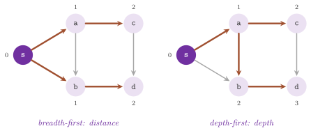
Figure 9.1 shows, on the left, the tree and the distances of a breadth-first search. On the right, the tree of a depth-first search of the same digraph is the subject of the next section.
9.3 Depth-first search¶
The depth-first search advances from the last node reached along an arc not
yet scanned, and backtracks to the node it came from when the node has no such
arc left. Dfs implements it without recursion, by a stack \(K\) that holds,
for each node of the current path from the source, the next out-arc to scan
from it (Algorithm 9.2, where \(\mathit{top}\) is the index of the top of \(K\),
\(-1\) for an empty stack). A node is processed, in the sense of the
ProcessedMap, when the search backtracks from it. In Dfs, the value
dist( v ) is the depth of \(v\) in the tree of the search, i.e., the number of
arcs of the path of the tree from the source, and in general it is not a
distance in the digraph.
Algorithm 9.2 (Depth-first search with a stack
of arcs, Dfs).
addSource(s):                                  [the stack must be empty]
1  if not reached(s): reached(s) := true; pred(s) := INVALID
2     if s has an out-arc: top := top + 1; K[top] := its first out-arc; d(s) := top
3     else: processed(s) := true; d(s) := 0
processNextArc():
4  a = uv := K[top]
5  if not reached(v): reached(v) := true; pred(v) := a
6                     top := top + 1; K[top] := the first out-arc of v (or INVALID)
7                     d(v) := top; x := v
8  else: K[top] := the next out-arc of u (or INVALID); x := u
9  while top >= 0 and K[top] = INVALID:
10    processed(x) := true; top := top - 1
11    if top >= 0: x := source(K[top]); K[top] := the next out-arc of x (or INVALID)
12 return a
start():   while top >= 0: processNextArc()
The properties for which the depth-first search is used (Tarjan 1972) follow from the invariant of the stack and from the fact that a node stays on the stack until all that it can reach is visited.
Lemma 9.1. During the search from a source
\(s\), the sources of the arcs \(K[0],\dots,K[\mathit{top}]\) (or, for an arc
INVALID pushed at step 6, the node \(v\) of that step) are the nodes of the
path of the tree from \(s\) to the node of the top, in this order; they are the
nodes reached in this search and not processed, and the depth of the node of
\(K[i]\) is \(i\).
Proof. By induction on the steps: step 2 makes the path \((s)\) with depth 0;
step 6 extends it by the head \(v\) of the arc \(a\) out of the node of the top,
which becomes the arc pred( v ) of the tree, with depth \(\mathit{top}\);
steps 8 to 11 change only the arc of the top, or remove the top node, which is
then marked processed. No other node is marked processed. \(\square\)
Lemma 9.2. Let \(v\) be reached when the set of the unreached nodes is \(U\). Then each node \(w\) that is reachable from \(v\) by a path whose nodes after \(v\) are in \(U\) is reached while \(v\) is on the stack, i.e., before \(v\) is processed, and is a descendant of \(v\) in the tree.
Proof. Let \(v=x_0,x_1,\dots,x_k=w\) be such a path, and suppose that some \(x_i\) is not reached while \(v\) is on the stack; let \(i\ge 1\) be the least such index. Then \(x_{i-1}\) is reached while \(v\) is on the stack, and therefore, by Lemma 9.1, it is above \(v\) on the stack and processed before \(v\). Before \(x_{i-1}\) is processed, all its out-arcs are scanned (steps 8 and 11 move to the next arc only after scanning one), the arc \(x_{i-1}x_i\) among them; hence, \(x_i\) is reached before \(v\) is processed, and after \(v\) is reached, since it was in \(U\), a contradiction. A node reached while \(v\) is on the stack is pushed above \(v\), and its path of the tree passes through \(v\) by Lemma 9.1. \(\square\)
Theorem 9.2. (i) The search from a source \(s\)
reaches exactly the nodes reachable from \(s\) through nodes not reached before
it, and takes \(O(1)\) time per node reached and per arc scanned, i.e.,
\(O(n+m)\) for run(). (ii) An arc \(uv\) is scanned while \(v\) is on the stack
only if \(G\) has a directed cycle through \(uv\); conversely, if \(G\) has a
directed cycle, run() scans such an arc. (iii) If \(G\) is acyclic, the
reverse of the order in which run() processes the nodes is a topological
order, i.e., the source of each arc precedes its target.
Proof. (i) follows from Lemma 9.2 applied to \(s\), and from the fact that each step either pushes a node, which happens once per node, or advances the arc of the top, which happens once per arc. For (ii), if \(v\) is on the stack when \(uv\) is scanned, then \(u\) is the top node, a descendant of \(v\) by Lemma 9.1, and the path of the tree from \(v\) to \(u\) and the arc \(uv\) form a cycle. Conversely, let \(C\) be a directed cycle and \(v\) its first node reached, and let \(uv\) be the arc of \(C\) entering \(v\). By Lemma 9.2, \(u\) is reached while \(v\) is on the stack, and the arc \(uv\) is scanned before \(u\) is processed, i.e., while \(v\) is still on the stack. For (iii), let \(uv\) be an arc. It is scanned when \(u\) is the top node, before \(u\) is processed. If \(v\) is not reached at that moment, it is pushed above \(u\) and processed before \(u\); if it is reached and not processed, it is on the stack (Lemma 9.1), and \(G\) has a cycle by (ii); otherwise it is already processed. Hence, \(v\) is processed before \(u\), and \(u\) precedes \(v\) in the reverse order. \(\square\)
The stack is a vector of \(n\) places, allocated by init(). Otherwise, the
interface follows §9.1, with three differences. First, the unit of
work is an arc: processNextArc() scans the arc on the top of the stack and
returns it, and nextArc() returns the next arc to be scanned, as an
OutArcIt (INVALID if the stack is empty), while queueSize() is the
height of the stack. Second, addSource() requires an empty stack (checked by
LEMON_DEBUG), since a source added to a search in progress would break the
invariant of Lemma 9.1; this is why run() adds each new source only after
the previous search has finished, and why the depths of run() are right in
every search. Third, the stopping condition of start( am ) is an arc map,
not a node map: the search stops before scanning an arc \(a\) with am[a] true
and returns it, or returns INVALID if the search ends first. Also,
start( t ) and run( s , t ) stop as soon as t is reached (at once, if
t is the source), and run( s , t ) returns reached( t ).
9.4 Function-type interfaces¶
The functions bfs( g ) and dfs( g ) return a BfsWizard and a DfsWizard
on the digraph g. Their members set the maps of the algorithm and the
outputs, each returning a new wizard, and their run() runs a Bfs or a
Dfs with them. Named function parameters predMap( m ), distMap( m ),
reachedMap( m ) and processedMap( m ) pass the maps that the algorithm
fills. Their types are deduced from the arguments, so that any writable map
may be passed, e.g., a LoggerBoolMap (cf. chapter 6) that
records the nodes in the order of processing. For a search between two nodes,
path( p ) gives a path into which the path to the target is copied, and
dist( d ) an int variable that receives its distance or depth (which, by
the remark of §9.1, is undefined when the target is not reached).
Three runs are available: run( s ), run( s , t ), which returns whether
t was reached and fills the path and the distance, and run(), which visits
all the nodes (as run() of the classes, with the same distances). Maps not
given are allocated by the algorithm for the duration of the run, and the path
given to path() may be of any path type that a path dumper can be assigned
to (by default a Path). The classes BfsWizardBase and DfsWizardBase hold
the pointers to the parameters, and the traits BfsWizardDefaultTraits and
DfsWizardDefaultTraits their default types; none of them is used directly.
Two typical calls are the following.
bool found = bfs(g).path(p).dist(d).run(s, t);
dfs(g).processedMap(loggerBoolMap(std::back_inserter(order))).run();
9.5 Visitors¶
BfsVisit< GR , VS , TR > and DfsVisit< GR , VS , TR > perform the same
searches as Bfs and Dfs. However, in place of filling a predecessor and a
distance map, they call a member of a visitor object of type VS at each
event of the search; the visitor is given to the constructor together with the
digraph. They keep only a ReachedMap (a NodeMap< bool > by default, given
by the traits BfsVisitDefaultTraits and DfsVisitDefaultTraits, and set by
reachedMap() or by the named parameter SetReachedMap< T >). Their
execution control is that of Bfs and Dfs (init(), addSource(),
processNextNode() or processNextArc(), nextNode() or nextArc(),
emptyQueue(), queueSize(), the three start() and the three run()), and
their only query is reached( v ). In the library, the visitors
BfsVisitor< GR > and DfsVisitor< GR > define the events as members with an
empty body, and a concept check of the members that a visitor must have. A
visitor of the user may derive from them, and redefine only the members it
needs.
BfsVisit calls start( s ) for each source and reach( v ) when a node is
reached for the first time (a source included). It calls process( u ) when a
node is taken from the queue, discover( a ) when an arc reaches a node not
yet reached (followed by reach() of its target), and examine( a ) when an
arc is scanned whose target was already reached. DfsVisit calls start( s )
and stop( s ) when the search from the source s begins and ends, and
reach( v ), discover( a ) and examine( a ) as BfsVisit does. It also
calls leave( v ) when the search backtracks from a node (the moment at which
Dfs marks it processed), and backtrack( a ) when the search returns along
the arc a of the tree to its source. Thus, reach() and leave() delimit
the time during which a node is on the stack, and an examine( a ) whose
target is on the stack reveals a directed cycle by Theorem 9.2 (ii). Note that
DfsVisit::nextArc() returns an Arc, while Dfs::nextArc() returns an
OutArcIt.
The program manual/examples/09-search.cc (the test manual_09_search)
computes the distances of a breadth-first search, a shortest path by bfs()
and a topological order by the order of processing of dfs() (Theorem 9.2
(iii)), and finds a directed cycle by a visitor of DfsVisit that keeps the
nodes on the stack between reach() and leave().
9.6 Maximum cardinality search¶
The maximum cardinality search orders the nodes of a graph so that each node,
when it is chosen, has the largest number of neighbours among those already
chosen. In abLEMON, MaxCardinalitySearch< GR , CAP , TR > extends it to
capacities \(c(a)\) on the arcs. The cardinality of an unprocessed node \(u\) is
and at each step the algorithm processes an unprocessed node of largest
cardinality among those with at least one arc into the processed nodes
(Algorithm 9.3), recording its cardinality at that moment. On a digraph the
sum (9.1) is over the arcs from \(u\) to the processed nodes, since the
algorithm scans the in-arcs of the node it processes. On an undirected graph
it is over the edges that join \(u\) to processed nodes; with unit capacities,
\(\kappa(u)\) is then the number of processed neighbours of \(u\). When the heap
becomes empty, i.e., when no unprocessed node has an arc into a processed
one, run() takes a new source among the nodes not reached.
Algorithm 9.3 (Maximum cardinality search,
MaxCardinalitySearch).
init():            H := empty heap of maximum priority; no node processed
addSource(s, p):   if s was never in H: push s with priority p (0 by default)
processNextNode():
1  u := the node of largest priority in H; cardinality(u) := its priority
2  processed(u) := true; pop u
3  for each arc wu entering u:
4     if w was never in H: push w with priority c(wu)
5     else if w is in H: increase the priority of w by c(wu)
6  return u
start():           while H is not empty: processNextNode()
run():             init(); for each node s not reached: addSource(s); start()
Theorem 9.3. In a search from a source added
with priority 0, the priority of each node \(w\) in \(H\) is \(\kappa(w)\) of
(9.1), so that each node, when processed, has the largest cardinality among
the unprocessed nodes that have an arc into the processed ones, and its
cardinality() is its cardinality at that moment. The search takes
\(O(n+m)\) time with unit capacities and the default BucketHeap, and
\(O(m\log n)\) with the BinHeap of the other capacities.
Proof. A node \(w\) enters \(H\) when the first node \(u\) with an arc \(wu\) is
processed, with the priority \(c(wu)\), and its priority grows by \(c(wu')\)
whenever another such node \(u'\) is processed (a parallel arc counting once
for each copy); hence, it is \(\kappa(w)\) at each moment, and the heap gives
its maximum. Each node is pushed and popped once, and each arc causes at most
one increase, when its head is processed. With a BinHeap, each operation
takes \(O(\log n)\). With unit capacities, the priorities are integers between
0 and \(m\), and a BucketHeap of maximum priority does each push and increase
in \(O(1)\), while the pointer to the largest bucket, which moves down over the
empty buckets at the pops, has moved up at most once per increase; hence, the
total is \(O(n+m)\) (§7.4). \(\square\)
With unit capacities, the order of the search recognizes the chordal graphs, i.e., those in which every cycle of four or more nodes has a chord. An order \(v_1,\dots,v_n\) of the nodes is a perfect elimination order if, for each \(i\), the neighbours of \(v_i\) that follow it form a clique.
Theorem 9.4. Let \(G\) be an undirected graph,
and let \(v_1,\dots,v_n\) be the order in which run() with unit capacities
processes its nodes. Then \(G\) is chordal if and only if, for each \(i\), the
neighbours of \(v_i\) among \(v_1,\dots,v_{i-1}\) form a clique, i.e., if and only
if \(v_n,\dots,v_1\) is a perfect elimination order.
Proof sketch. If the condition holds, let \(C\) be a chordless cycle of at least four nodes, and \(v_i\) its last node in the order: its two neighbours on \(C\) come before it and must be adjacent, which is a chord. Conversely, the key property of the order is that, if \(a\) precedes \(b\), \(b\) precedes \(c\), \(ac\in E\) and \(ab\notin E\), then some \(d\) before \(b\) has \(db\in E\) and \(dc\notin E\): indeed, when \(b\) was chosen, its count of processed neighbours was at least that of \(c\), which includes \(a\). Starting from a violation of the condition, i.e., two nonadjacent earlier neighbours of some \(v_i\), and applying this property repeatedly to the extreme pair, one builds longer and longer chordless paths whose ends precede all their inner nodes, which in a chordal graph cannot go on, since a finite graph has no infinite such sequence. The complete argument is in Tarjan and Yannakakis 1984, section 2. \(\square\)
Thus, chordality can be tested in linear time, by checking the condition of Theorem 9.4 on the order as in Tarjan and Yannakakis 1984 (the program of this section implements a simpler and slower version of the check, pair by pair). With general capacities, the order is a maximum adjacency order, which the algorithm of Nagamochi and Ibaraki (§15.3) needs.
Its template parameters are the graph type GR, the type CAP of the map of
the capacities, by default ConstMap< GR::Arc , Const< int , 1 > > (unit
capacities), and the traits class TR, by default
MaxCardinalitySearchDefaultTraits< GR , CAP >. Its traits give Digraph,
the CapacityMap and its Value, the CardinalityMap (a NodeMap of
Value), the ProcessedMap (a NullMap by default), the HeapCrossRef (a
NodeMap< int >) and the Heap, each with its function create...(). The
heap is a BucketHeap of maximum priority for the unit capacities, and a
BinHeap with std::greater, i.e., again of maximum priority, otherwise; the
internal templates CapMapSelector, HeapSelector and Selector of the
traits make this choice and create the map of unit capacities. Named
parameters SetCapacityMap< T >, SetCardinalityMap< T >,
SetProcessedMap< T > and SetHeap< H , CR > change these types and require
the map, or the heap, to be given by the corresponding setter;
SetStandardHeap< H , CR > changes the type of the heap, which the algorithm
then allocates with its cross reference map.
Its constructor takes the graph and the capacity map, or only the graph, in
which case the traits create the map, i.e., the map of unit capacities by
default, or a map of type CAP constructed on the graph (with the default
values of its constructor) otherwise. Its setters are capacityMap( m ),
cardinalityMap( m ), processedMap( m ) and heap( hp , cr ), and the
readers capacityMap(), processedMap(), heap(), heapCrossRef() and
cardinalityMap() return the maps and the heap in use. Its execution control
is made of init(), addSource( s , capacity ), processNextNode(),
nextNode(), emptyQueue() and emptySize(), which, despite its name, is
the number of nodes in the heap. Searches are run by start(), run( s ),
run(), and start( dest ) and start( nm ); the last two stop when dest,
or a node with nm true, is on the top of the heap, and write its cardinality
(and true into the ProcessedMap) without removing it from the heap, so
that processed() stays false for it.
Its queries are cardinality( v ), i.e., the cardinality of \(v\) when it was
processed (undefined for a node never processed), currentCardinality( v ),
its priority in the heap (for a node reached but not processed), and
cardinalityMap(). Also, reached( v ) is true if \(v\) has ever been in the
heap, and processed( v ) if it has left it.
The program manual/examples/09-max-cardinality.cc (the test
manual_09_max_cardinality) runs the search step by step on a chordal graph
and on a chordless cycle of four nodes, records the order, and checks the
condition of Theorem 9.4, which holds on the first graph and fails on the
second, together with the cardinalities given by the algorithm.
9.7 Exercises¶
Exercise 9.1. Run Bfs from several sources
added with addSource() and show that dist( v ) is the distance from the
nearest source; compare with a single search from a new node joined by an arc
to each source. (The test test/bfs_test.cc exercises the interface of
Bfs.)
Exercise 9.2. Use Bfs on an undirected graph to
test whether it is bipartite, by checking that no edge joins two nodes at the
same distance from the source of their component, as run() gives them;
compare the answer with bipartite() of chapter 18, and explain why the
levels must start again from 1 at each new source (cf. the remark after
Theorem 9.1).
Exercise 9.3. Write a visitor of DfsVisit that
numbers the nodes in preorder and in postorder, and use the two numbers to
classify the arcs into tree, back, forward and cross arcs; check that a
digraph is acyclic if and only if there is no back arc. (The program
manual/examples/09-search.cc detects the back arcs; the test
test/dfs_test.cc exercises Dfs and DfsVisit.)
Exercise 9.4. Stop a Dfs by start( am ) at
the first arc whose target is on the current path, with an arc map computed on
the fly from the ReachedMap and the ProcessedMap; explain why a node map
would not suffice for this, which is why start() of Dfs takes an arc map.
Exercise 9.5. Run MaxCardinalitySearch with the
capacities of the edges of a graph, and verify that the cardinality of the
last node processed, \(t\), equals the capacity of a minimum cut between \(t\) and
the node \(s\) processed just before it (the lemma behind the algorithm of
Nagamochi and Ibaraki), by comparing it with Preflow of chapter 12. (The
test test/max_cardinality_search_test.cc checks the cardinalities on a small
digraph.)