20. The LP and MIP interface¶
This chapter describes the interface through which a program builds a Linear
Program (LP) or a Mixed Integer Program (MIP) and has it solved by an external
solver. The interface is declared in lp_base.h, the default solvers are
chosen in lp.h, the skeletons of lp_skeleton.h do nothing but compile, and
glpk.h, cplex.h, clp.h, cbc.h and soplex.h connect the interface to
GLPK, CPLEX, Clp, Cbc and SoPlex. Unlike the rest of the library, these
classes are not templates: they are compiled into the library, each backend
only when its solver is found at configuration time (chapter
2). A program written against the base classes
compiles with any backend; it also compiles with none, although then only the
skeletons are available.
20.1 The structure of the interface¶
We are concerned with problems of the form
where \(x\in\mathbb{R}^n\) are the columns, \(A\) is an \(m\times n\) matrix whose
row \(i\) has the bounds \(l^r_i\in\mathbb{R}\cup\{-\infty\}\) and
\(u^r_i\in\mathbb{R}\cup\{+\infty\}\), and each column \(j\) has the bounds
\(l^c_j\) and \(u^c_j\) alike. Also, \(c\in\mathbb{R}^n\) is the vector of the
objective coefficients, \(c_0\) is a constant, and \(J\) is the set of the integer
columns, which is empty for an LP. A row with \(l^r_i=u^r_i\) is an equation,
and one with both bounds finite is a range constraint. The interface
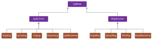
describes (20.1) with three classes (Figure 20.1): LpBase holds the model,
i.e., the columns, the rows, the coefficients, the bounds and the objective;
LpSolver adds the solution of an LP, with its dual values and its basis;
MipSolver adds the integrality of the columns and the solution of a MIP.
Both LpSolver and MipSolver derive virtually from LpBase, and a backend
derives from one of them. Hence, a function that takes an LpSolver & works
with any LP backend, and one that takes an LpBase & builds a model for both
kinds of solvers.
All the numbers of the interface are of the type LpBase::Value, which is
double. The constants LpBase::INF and LpBase::NaN are the infinity and
the quiet NaN of double; an infinite bound is written as INF or -INF,
and NaN marks an unset bound of a constraint (§20.2). The
enumerations of LpBase are Sense (MIN, MAX), MessageLevel
(MESSAGE_NOTHING, MESSAGE_ERROR, MESSAGE_WARNING, MESSAGE_NORMAL,
MESSAGE_VERBOSE) and SolveExitStatus. The last is the value returned by
solve(): it is SOLVED (0) when the solver has found an optimal solution or
proved the problem infeasible or unbounded, and UNSOLVED (1) in any other
case, e.g., when a limit of the solver stopped it. Whether a solved problem is
optimal, infeasible or unbounded is then read from the problem type
(§20.4 and §20.5).
Then lp.h defines the default solvers. When at least one backend is found at
configuration time, the macro LEMON_HAVE_LP (and, for GLPK, CPLEX and Cbc,
LEMON_HAVE_MIP) is defined in lemon/config.h, together with
LEMON_HAVE_GLPK, LEMON_HAVE_CPLEX, LEMON_HAVE_CLP, LEMON_HAVE_CBC and
LEMON_HAVE_SOPLEX for the backends found. In this case Lp is the default
LP solver, and Mip the default MIP solver, chosen by the macros
LEMON_DEFAULT_LP (one of LEMON_GLPK_, LEMON_CPLEX_, LEMON_SOPLEX_,
LEMON_CLP_) and LEMON_DEFAULT_MIP (one of LEMON_GLPK_, LEMON_CPLEX_,
LEMON_CBC_), which lp.h maps to the classes of the backends and whose
headers it includes. Usually the CMake options LEMON_DEFAULT_LP and
LEMON_DEFAULT_MIP choose them; when they are not given, or they name a
solver that was not found, the first solver found is taken in the order CPLEX,
Clp (with Cbc for the MIP), GLPK, SoPlex. SoPlex is an LP solver only, and
therefore Mip is not defined when it is the only backend; neither Lp nor
Mip is defined when no backend is found. A program that must compile in all
cases guards their use with #ifdef LEMON_HAVE_LP and #ifdef
LEMON_HAVE_MIP, as test/lp_test.cc and test/mip_test.cc do, and as the
program of §20.8 does.
20.2 Columns, rows and expressions¶
A column (a variable) is referred to by an object of the class LpBase::Col,
and a row (a constraint) by an object of LpBase::Row. These handles behave
as the items of a graph (chapter 3): they are
copied freely, they compare with ==, != and < (an artificial order, for
the associative containers), a default constructed one is undefined, and one
constructed from INVALID is invalid. The static functions id( col ),
colFromId( id ), id( row ) and rowFromId( id ) convert between a handle
and its integer id. The iterators ColIt and RowIt, constructed from the
solver, list the columns and the rows in the order of their addition, and the
non-constant functions cols() and rows() return ranges for the loops of
C++11. The handles stay valid when other columns or rows are added or erased,
since LpBase keeps, for the columns and for the rows, its own index (the
class VarIndex of bits/solver_bits.h) between the ids of the handles and
the indices of the solver.
Lemma 20.1. The id of a handle does not change while its column or row exists, and the index translates it into the current index of the solver in \(O(1)\) time. Adding a column or a row costs \(O(1)\) amortized time in the index; erasing one costs \(O(1)\), plus \(O(k)\) for the backends whose solver renumbers the following \(k\) columns or rows (GLPK, Clp and CPLEX); SoPlex moves the last column or row into the place of the erased one, in \(O(1)\). The id of an erased column or row is reused by the next one added.
Proof. The index keeps a vector of records, one per id, linked in a list in
the order of addition (the order of ColIt and RowIt) and holding the index
of the solver, and a vector cross from the indices of the solver to the ids.
Adding takes the first record of a list of free ids, or a new one at the end
of the vector, and sets both directions in \(O(1)\) (amortized, for the growth
of the vectors). Erasing unlinks the record and puts it at the head of the
free list, which is why its id is reused next. When the solver shifts down the
indices that follow the erased one, shiftIndices() moves the entries of
cross and decreases the indices stored in their records, in time
proportional to their number, and when it moves the last one into the hole,
relocateIndex() updates one entry. The id of the other handles is never
changed. \(\square\)
Hence, a handle of an erased column must not be used afterwards, since it may
refer to the column added next. A linear expression of the columns with a
constant term is an object of the class LpBase::Expr, whose Key is Col
and whose Value is double. It stores the nonzero coefficients in a
std::map from the column id to the value, and the constant apart, so that an
access to a coefficient costs \(O(\log k)\) for an expression of \(k\) terms. A
number and a column convert implicitly to an Expr, and the binary operators
+, -, * and / by a number, with their compound forms, combine
expressions (there is no unary minus, and one writes -1 * x). For instance,
2 * x + 3 * (y - x) + 4 is the expression \(-x+3y+4\). The coefficient of a
column is read with e[c] (zero when absent) and changed through the
reference returned by the non-constant e[c], and the constant term is
accessed by the unary *e. Also, clear() sets everything to zero, and
simplify( eps ) removes the coefficients whose absolute value is at most
eps (by default 0) and sets the constant to zero under the same condition.
The iterators CoeffIt and ConstCoeffIt list the terms in the order of the
ids, converting to the column of the term and dereferencing to its
coefficient. Note that set(c, v) removes the term when v is zero, and
otherwise gives the column the coefficient v, as e[c] = v does.
abLEMON
In LEMON 1.3.1, Expr::set() and DualExpr::set() called
std::map::insert, and therefore left an existing coefficient unchanged;
the test lp_test checks that they replace it.
A constraint is an object of the class LpBase::Constr, made of an expression
and of a lower and an upper bound, read and written by expr(),
lowerBound() and upperBound(); lowerBounded() and upperBounded() tell
whether a bound is set and finite, and clear() empties the expression and
unsets both bounds. A bound equal to NaN is unset, which is the state of both
bounds of a default constructed constraint and of one constructed from an
expression alone. The comparison operators between expressions and numbers
build constraints, as Table 20.1 shows.
| Written | Lower bound | Expression | Upper bound |
|---|---|---|---|
e <= s |
unset | e |
s |
s <= e |
s |
e |
unset |
e <= f |
0 | f - e |
unset |
e == s |
s |
e |
s |
e == f |
0 | f - e |
0 |
(s <= e) <= t |
s |
e |
t |
Table 20.1. The constraints built by the
comparison operators, e and f expressions (or columns) and s and t
numbers; >= gives the mirrored cases, and s == e is taken as e == f with
f the constant s.
A second bound can be added to a constraint by comparing it with a number, as
in the last row of Table 20.1, but only on the side that is still unset. This
is checked at run time by LEMON_ASSERT (when assertions are enabled,
chapter 8), and hence (e <= 5) <= 6 compiles but
fails the assertion. Since C++ evaluates s <= e <= t as (s <= e) <= t, the
form -3 <= v <= 4 builds the range constraint intended. We remark that a
chain of two expressions and a number is valid too: x <= y <= 5 is
(x <= y) <= 5, i.e., the range constraint \(0\le y-x\le 5\), which passes the
assertion.
Similarly, LpBase::DualExpr is the analogous expression of the rows, i.e., a
column of the matrix, or a linear combination of the dual variables; its Key
is Row, it has the same members as Expr except the constant term, and the
same operators. Rows convert to it implicitly, and it is used to set or read a
whole column (§20.3) and to evaluate a combination of the
dual values (§20.4).
20.3 Building and modifying a problem¶
We now describe the members of LpBase that build and change the model. All
of them work through the virtual functions of the backend, and therefore their
cost is the one of the solver, besides the \(O(1)\) of the index (Lemma 20.1)
and the \(O(k\log k)\) of an expression of \(k\) terms. A column is added by
addCol(), which gives an empty column with the bounds \(-\infty\) and
\(+\infty\) in all the backends of the library, and by addCol( e , o ), which
also sets its coefficients from the DualExpr e and its objective
coefficient to o (0 by default). The function addColSet( t ) fills a
container with new columns and returns their number. The argument t can be a
container of Col (e.g., a std::vector), an associative container whose
mapped type is Col (e.g., a std::map< K , Col >), or a writable map of the
library with values of type Col, e.g., a
ListDigraph::ArcMap< LpBase::Col >, which gives one column per arc. The rows
are added in the same ways: addRow() gives an empty row, addRowSet( t )
fills a container, and addRow( l , e , u ) and addRow( c ) add a row from
an expression with two bounds or from a constraint.
When an expression with constant term \(c_e\) enters a row, the constant is
moved to the bounds, i.e., the row \(l\le a^\top x+c_e\le u\) is stored as
\(l-c_e\le a^\top x\le u-c_e\). In addRow( c ) and row( r , c ) from a
constraint, an unset or infinite bound becomes \(\mp\infty\) first, while
addRow( l , e , u ) and row( r , l , e , u ) pass the given bounds as they
are (and so pass a NaN to the solver). The functions that take an expression
(addRow(), row(), addCol( e , o ) and col()) first remove its zero
coefficients, which they do in the expression of the caller, although they
take it by constant reference.
Once created, a column is changed by col( c , e ), which sets its
coefficients, and read back as a DualExpr by col( c ); the analogous
row( r , l , e , u ) and row( r , c ) set a row, and row( r ) returns
its coefficients as an Expr. A single coefficient is set and read by
coeff( r , c , v ) and coeff( r , c ), and erase( c ) and erase( r )
remove a column or a row. The bounds are set and read by
colLowerBound( c , v ), colUpperBound( c , v ), colBounds( c , l , u ),
rowLowerBound( r , v ) and rowUpperBound( r , v ), with the getters
colLowerBound( c ), colUpperBound( c ), rowLowerBound( r ) and
rowUpperBound( r ); the three column setters also accept a container or a
map of columns, as addColSet() does, to give the same bounds to all of them.
Names are given by colName( c , s ) and rowName( r , s ), read by
colName( c ) and rowName( r ), and searched by colByName( s ) and
rowByName( s ), which return INVALID when no item has the name.
The objective is set by obj( e ), which replaces all the coefficients and
whose constant term is kept by LpBase itself and added to the objective
value of the solution, and read by obj(); objCoeff( c , v ) and
objCoeff( c ) set and read one coefficient. The direction is set by
sense( MIN ) or sense( MAX ), or by the shorthands min() and max(),
and read by sense(). Finally, clear() empties the model, the index of the
columns and of the rows, and the constant term of the objective,
messageLevel( level ) sets how much the solver prints (all the backends
start at MESSAGE_NOTHING), and solverName() returns the name of the
backend. Also, write( file , format ) writes the model to a file, by default
in the format "MPS"; a format that the backend does not support throws
LpBase::UnsupportedFormatError, an Exception whose what() names the
format (Table 20.2).
abLEMON
In LEMON 1.3.1, clear() kept the constant term of the objective, which
primal() and solValue() went on adding until the next obj( e ); the
test lp_skeleton_test checks that it is reset.
20.4 Solving an LP and reading the solution¶
For an LP, i.e., (20.1) with \(J=\emptyset\), the class LpSolver adds the
solution. We recall the optimality conditions that its dual values satisfy,
for a minimization (for a maximization, one minimizes \(-c^\top x\)). For
\(y\in\mathbb{R}^m\), let \(d=c-A^\top y\) be the vector of the reduced costs, and
let
where a minimum is \(-\infty\) when it is unbounded, e.g., when \(y_i>0\) and \(l^r_i=-\infty\). The dual problem is \(\max\{\varphi(y):y\in\mathbb{R}^m\}\), and a \(y\) with \(\varphi(y)>-\infty\) is dual feasible.
Lemma 20.2. For every \(x\) feasible for (20.1) with \(J=\emptyset\) and every \(y\), \(c^\top x\ge\varphi(y)\), with equality if and only if
Proof. One has \(c^\top x=y^\top Ax+d^\top x=\sum_i y_i(Ax)_i+\sum_j d_jx_j\). Since \((Ax)_i\in[l^r_i,u^r_i]\) and \(x_j\in[l^c_j,u^c_j]\), each term is at least the corresponding minimum of (20.2), and the sum is at least \(\varphi(y)\). Equality holds if and only if each term attains its minimum; the minimum of \(y_is\) over the interval is attained at the lower end when \(y_i>0\), at the upper end when \(y_i<0\), and anywhere when \(y_i=0\), and likewise for \(d_jt\), which gives (20.3). \(\square\)
Theorem 20.1. A feasible \(x\) is optimal for (20.1) with \(J=\emptyset\) if and only if there is a \(y\) that satisfies (20.3), and then \(y\) is optimal for the dual problem.
Proof. If \(y\) satisfies (20.3), then \(c^\top x=\varphi(y)\le c^\top x'\) for every feasible \(x'\) by Lemma 20.2, and \(\varphi(y')\le c^\top x=\varphi(y)\) for every \(y'\). Conversely, if \(x\) is optimal, the strong duality theorem of linear programming, applied to (20.1) written with the inequalities \(Ax\ge l^r\), \(-Ax\ge-u^r\), \(x\ge l^c\) and \(-x\ge-u^c\) (the infinite ones dropped), gives nonnegative multipliers of the four groups whose dual objective equals \(c^\top x\). The differences of the multipliers of the two rows of each pair form a \(y\) with \(\varphi(y)\ge c^\top x\), and hence \(\varphi(y)=c^\top x\), which gives (20.3) by Lemma 20.2. The strong duality theorem is proved, e.g., in Bertsimas and Tsitsiklis 1997, §4.3, Theorem 4.4, and in Dantzig 1963. \(\square\)
In the classical interpretation of the multipliers, the dual value \(y_i\) of a row is the rate of change of the optimal value with respect to the bound that is active, and by (20.3) its sign indicates which bound it is. The interface passes on the dual values of the solver unchanged, and hence their sign convention, in particular for a maximization, is the one of the solver.
A call of solve() solves the problem and returns the SolveExitStatus of
§20.1. The problem type of the primal and of the dual
problem is then read by primalType() and dualType(), of the enumeration
LpSolver::ProblemType: UNDEFINED (no feasible solution found, although one
may exist), INFEASIBLE, FEASIBLE (a feasible solution found, its
optimality not proved), OPTIMAL and UNBOUNDED. The values of a solution
are read by primal( c ) for a column, primal( e ) for an expression (the
scalar product with the primal solution plus the constant term), dual( r )
for a row and dual( e ) for a DualExpr; all of them require a solved
problem. As for the objective value, primal() includes the constant term of
the objective; according to the documentation, it is INF or -INF for an
infeasible or unbounded problem, depending on the direction, and NaN when no
primal solution is found. Also, the basis is read by colStatus( c ) and
rowStatus( r ), of the enumeration VarStatus: BASIC, FREE (nonbasic
and free), LOWER and UPPER (nonbasic at a bound) and FIXED (nonbasic and
fixed).
When the problem has no optimal solution, the rays certify it, in the backends that provide them (the header warns that some solvers do not compute them). Let \(\varphi_0\) be the function (20.2) with \(c\) replaced by \(0\), i.e., the dual problem with its right-hand sides set to 0.
Lemma 20.3. (i) Let \(r\) satisfy the bounds of (20.1) with each finite bound replaced by 0 and the infinite ones kept, i.e., \((Ar)_i\ge0\) if \(l^r_i\) is finite, \((Ar)_i\le0\) if \(u^r_i\) is finite, and likewise for \(r_j\), and let \(c^\top r<0\) (a primal ray). Then the dual problem has no feasible \(y\), and if (20.1) has a feasible \(x\), it is unbounded. (ii) Let \(w\) satisfy \(\varphi_0(w)>0\) (a dual ray). Then (20.1) is infeasible.
Proof. (i) Let \(\varphi(y)>-\infty\). If \(y_i>0\) then \(l^r_i\) is finite, since otherwise the \(i\)-th minimum of (20.2) is \(-\infty\), and so \((Ar)_i\ge0\); if \(y_i<0\), then \(u^r_i\) is finite and \((Ar)_i\le0\). Hence \(y_i(Ar)_i\ge0\) for every \(i\), and in the same way \(d_jr_j\ge0\) for every \(j\). Then \(c^\top r=y^\top Ar+d^\top r\ge0\), a contradiction. If \(x\) is feasible, so is \(x+tr\) for every \(t\ge0\), since a finite bound that \(x\) satisfies stays satisfied along \(r\) and the infinite ones impose nothing, and \(c^\top(x+tr)\to-\infty\). (ii) If \(x\) were feasible, Lemma 20.2 with \(c=0\) would give \(0=0^\top x\ge\varphi_0(w)>0\), which is impossible. \(\square\)
In the interface, primalRay( c ) gives the component of a primal ray on the
column \(c\), with a negative objective value for a minimization and a positive
one for a maximization. Similarly, dualRay( r ) gives the component of a
dual ray on the row \(r\); the first requires that the dual problem be
infeasible, and the second that the primal problem be infeasible. Finally,
newSolver() returns a new empty solver of the same type, and cloneSolver()
a copy of the problem; both return a pointer that the caller deletes.
20.5 Mixed integer programs¶
In MipSolver one describes (20.1) with integer columns. The type of a column
is set by colType( c , type ) and read by colType( c ), of the enumeration
MipSolver::ColTypes: REAL (the default) or INTEGER; a binary column is
an integer one with the bounds 0 and 1. As for an LP, solve() returns
SOLVED or UNSOLVED, and type() returns the problem type, of the
enumeration MipSolver::ProblemType, with the same five values as
LpSolver::ProblemType; UNBOUNDED means that the MIP, or at least its
continuous relaxation, is unbounded. The solution is read by sol( c ),
sol( e ) and solValue(), the last one including the constant term of the
objective. A MIP solver gives no dual values and no basis, and its
newSolver() and cloneSolver() return a MipSolver *.
The integrality of a column whose bounds are not integer deserves a remark
(cf. Exercise 20.5). The integer values of such a column are those of \([\lceil
l^c_j\rceil, \lfloor u^c_j\rfloor]\), and the problem is infeasible when this
interval is empty. GLPK refuses such a column, and Cbc does not round its
bounds; hence, GlpkMip and CbcMip round the bounds of each integer column
inwards before the solve, up to an integer tolerance \(\epsilon=10^{-6}\), as in
Algorithm 20.1, which is the one of GlpkMip::_solve().
Algorithm 20.1 (The solve of GlpkMip).
1  solve the continuous relaxation by the dual simplex method
   (on a bad, singular or ill-conditioned basis, build an advanced basis by
   glp_adv_basis() and solve once more; return UNSOLVED if this fails)
2  if the relaxation is not optimal: return SOLVED (type: of the relaxation)
3  for each integer column j, until one without integer values is found:
4      l' := ceil(l_j - eps) if l_j is finite; u' := floor(u_j + eps) if u_j is
         finite
5      if both bounds are finite and l' > u': the problem is INFEASIBLE;
         skip the search
6      else give the column the bounds [l', u'] (fixed if l' = u')
7  run the branch and cut of GLPK (glp_intopt)
8  give back the bounds given by the user; return SOLVED, or UNSOLVED
   if glp_intopt failed
Theorem 20.2. Let \(Z_j=\{z\in\mathbb{Z}: l^c_j-\epsilon\le z\le u^c_j+\epsilon\}\) for each integer column \(j\). Algorithm 20.1 solves the MIP whose integer columns range over the sets \(Z_j\), i.e., (20.1) with each bound of an integer column relaxed by \(\epsilon\); it declares the problem infeasible, without calling the branch and cut, exactly when some \(Z_j\) is empty, and it leaves the bounds of the model as they were given. The rounding costs \(O(n)\) calls of GLPK.
Proof. For an integer \(z\) and a real \(l\), \(z\ge l-\epsilon\) holds if and
only if \(z\ge\lceil l-\epsilon\rceil\), and \(z\le u+\epsilon\) if and only if
\(z\le\lfloor u+\epsilon\rfloor\). Hence the integers of \([l',u']\) are \(Z_j\),
and the rounded MIP has the same feasible set as the relaxed one. When both
bounds are finite, \(Z_j\) is empty if and only if \(l'>u'\), and then the MIP has
no feasible solution, which line 5 records (the type is then INFEASIBLE); a
column with an infinite bound has a nonempty \(Z_j\). Line 8 restores the bounds
saved before they were changed, and each column is examined once. \(\square\)
CbcMip rounds the bounds in the same way in the copy of the problem that it
gives to Cbc, which leaves the bounds of the model unchanged, and a column
without integer values makes the initial solve of Cbc infeasible. The test
test/mip_test.cc checks both that the bounds stay as they were given and
that a column without integer values makes the problem infeasible.
abLEMON
The rounding of the bounds of the integer columns in GlpkMip and
CbcMip is new in abLEMON (version 1.4.1): GLPK 5.0 refused such a
column, which left the problem unsolved, and Cbc gave a solution beyond
the bound. Also, CbcMip no longer reports a proven infeasible problem as
feasible (trac #626, version 1.4.0).
20.6 The backends¶
Each backend wraps one solver and adds a few functions of its own. All of them have a default constructor and a copy constructor, which copies the problem. Table 20.2 summarizes them, and the paragraphs below give the details.
| Class | Solver | solve() |
Other solves | Formats of write() |
|---|---|---|---|---|
GlpkLp |
GLPK | primal simplex | solvePrimal(), solveDual() |
"MPS", "LP" |
GlpkMip |
GLPK | Algorithm 20.1 | "MPS", "LP" |
|
CplexLp |
CPLEX | CPXlpopt |
solvePrimal(), solveDual(), solveBarrier() |
"MPS", "LP", "SOL" |
CplexMip |
CPLEX | branch and cut of CPLEX | "MPS", "LP", "SOL" |
|
ClpLp |
Clp | primal simplex | solvePrimal(), solveDual(), solveBarrier() |
"LP" |
CbcMip |
Cbc | branch and cut of Cbc | none | |
SoplexLp |
SoPlex | simplex of SoPlex | none |
Table 20.2. The backends, the method of
solve(), the other solve functions, and the formats accepted by write();
any other format throws UnsupportedFormatError.
GLPK. GlpkLp and GlpkMip share the base GlpkBase, whose lpx()
returns the pointer to the problem object of GLPK (as a
_solver_bits::VoidPtr, which converts to any pointer type), and whose
lpxRow( r ) and lpxCol( c ) give the indices that GLPK uses. Each solve
function of GlpkLp runs the simplex method of GLPK; when it reports a bad,
singular or ill-conditioned basis, it builds an advanced basis by
glp_adv_basis() and runs once more, and it returns UNSOLVED if this fails
too. The function presolver( bool ) turns the presolver of GLPK on or off,
and it is off by default. Also, a static member of GlpkBase of the private
type FreeEnvHelper frees the environment of GLPK (glp_free_env()) when the
program ends.
CPLEX. CplexLp and CplexMip share the base CplexBase, whose
cplexEnv() and cplexLp() return the environment and the problem objects of
CPLEX, and whose env() returns the CplexEnv in use. A CplexEnv wraps the
environment of CPLEX with a reference count protected by a lock, so that
several problems can share one environment (and one license); it is copied and
assigned by sharing the environment. The constructors of CplexLp and
CplexMip that take a CplexEnv use the given one, and the others open a new
one. When the license check fails, the constructor of CplexEnv throws
CplexEnv::LicenseError, whose what() gives the message of CPLEX. In
CplexLp, solve() calls CPXlpopt, which lets CPLEX choose the method, and
the three other functions force the primal simplex, the dual simplex and the
barrier method.
Clp and Cbc. ClpLp wraps a ClpSimplex object of
Clp; solve() runs the primal simplex method,
and clpRow( r ) and clpCol( c ) give the indices of Clp. Note that ClpLp
writes only the format "LP", and therefore write( file ) with the default
"MPS" throws. CbcMip keeps the model in a CoinModel of
Cbc, and at each solve it copies the model into a
new OsiClpSolverInterface (with the rounding of §20.5)
and solves the continuous relaxation. When this is optimal, it runs the branch
and cut of Cbc with a fixed set of cut generators (probing, Gomory, knapsack
cover, odd hole, clique, mixed integer rounding and flow cover) and of primal
heuristics (rounding, local search, greedy cover, feasibility pump and RINS).
SoPlex. SoplexLp wraps the class SoPlex of
SoPlex. Its message level MESSAGE_NOTHING
maps to the verbosity of errors of SoPlex, which is (apparently) the lowest
one SoPlex offers. Its primal ray is the one of SoPlex, and its dual ray is
the Farkas proof of the infeasibility of the primal problem, i.e., a \(w\) of
Lemma 20.3 (ii).
abLEMON
SoplexLp works with SoPlex 5 and later, through the API of its class
SoPlex; in LEMON 1.3.1 it did not compile with these versions, and it
gave the Farkas proof of the dual as its primal ray (version 1.5.0).
SoPlex is found through its CMake configuration.
20.7 The skeletons¶
The header lp_skeleton.h declares LpSkeleton and MipSkeleton, which
derive from LpSolver and MipSolver and from the common base
SkeletonSolverBase. They implement the virtual functions of the interface by
doing (almost) no work. The coefficients, the bounds and the names are not
stored, the getters return 0 (or MIN for the sense, REAL for the type of
a column, an empty name, and -1, i.e., INVALID, for a search by name), and
solve() returns SOLVED. The
problem types are UNDEFINED, the basis statuses are BASIC, write()
writes nothing and throws nothing, and newSolver() and cloneSolver()
return a null pointer. Their names are "LpSkeleton" and "MipSkeleton". The
indices of the solver are counted from 0, and clear() starts them from 0
again. On a skeleton, however, all that LpBase keeps works as with a real
solver: the index of the columns and of the rows, and hence ColIt, RowIt,
cols(), rows() and the handles, and the classes Expr, DualExpr and
Constr with their operators, which do not involve the solver at all.
abLEMON
clear() of the skeletons starts the indices of the columns and of the
rows from 0 again, as the constructor does; in LEMON 1.3.1 they started
from 1 after a clear(). Also, in LEMON 1.3.1 MipSkeleton did not
implement _setColType() and _getColType(), and was an abstract class
that could not be instantiated; the test lp_skeleton_test builds one.
We see two uses of the skeletons. First, a program can build and check a
model, e.g., count its columns and rows, without any solver;
test/lp_skeleton_test.cc does so in all configurations, test/lp_test.cc
also when a backend is found, and so does the program of
§20.8. Second, they are the starting point for a new
backend. Such a backend must implement the pure virtual functions declared in
lp_base.h: _addCol(), _addRow(), _eraseCol(), _eraseRow(), the
functions of the names (_getColName(), _setColName(), _colByName() and
those of the rows), of the coefficients (_setRowCoeffs(), _getRowCoeffs(),
_setColCoeffs(), _getColCoeffs(), _setCoeff(), _getCoeff()), of the
bounds, of the objective (_setObjCoeffs(), _getObjCoeffs(),
_setObjCoeff(), _getObjCoeff()) and of the sense, _clear(),
_solverName() and _messageLevel(). An LP backend also implements
_solve(), the getters of the solution, of the rays, of the basis and of the
problem types, newSolver() and cloneSolver(); a MIP backend implements
_solve(), _setColType(), _getColType(), _getType(), _getSol(),
_getSolValue(), newSolver() and cloneSolver(). The coefficients reach
the backend through two protected iterators of LpBase: ExprIterator lists
the terms of an expression as pairs of a solver index and a value, and
InsertIterator stores the pairs returned by the solver into an expression,
translating the indices. The function _addRow( l , b , e , u ), which adds a
row with its coefficients and bounds in one call, has a default implementation
by _addRow() and the setters, and _write() one that throws
UnsupportedFormatError. The virtual functions _addColId(), _addRowId(),
_eraseColId() and _eraseRowId() update the index, and a backend whose
solver renumbers its columns or rows on an erasure overrides the last two to
call shiftIndices() (or, as SoplexLp does, relocateIndex()).
20.8 An example¶
The program manual/examples/20-lp.cc (the test manual_20_lp) writes the
maximum flow problem on a digraph \(G=(N,A)\) with capacities \(u\), a source \(s\)
and a sink \(t\) as the LP
Here \(\delta^+(v)\) and \(\delta^-(v)\) are the arcs leaving and entering \(v\).
The model is built in a function that takes any LpSolver, with one column
per arc obtained by addColSet() on an arc map and one row per inner node. It
builds the model on an LpSkeleton, on which it checks the number of columns
and rows and the algebra of the expressions and constraints of Table 20.1,
including a coefficient set twice by Expr::set(). When the library has an LP
backend, the same function builds the model on the default solver Lp, which
solves it, and the program compares the optimal value with the one of
Preflow (chapter 12). Without a backend this part is
left out by #ifdef LEMON_HAVE_LP, and the program still compiles and checks
the rest.
20.9 Exercises¶
Exercise 20.1. Write the shortest path problem
from \(s\) to \(t\) as an LP with one column per arc, solve it with the default
solver, and compare its value with the distance computed by Dijkstra
(chapter 10). Then read the dual values of the
rows and check that they are distances from \(s\) (up to a constant and to the
sign convention of the solver), as Theorem 20.1 predicts.
Exercise 20.2. Build an infeasible LP, e.g., by
adding to the model of (20.4) the row \(\sum_{a\in\delta^+(s)} x_a \ge 1+\sum_a
u_a\), and verify that primalType() is INFEASIBLE and that the dual ray,
when the backend provides it, satisfies Lemma 20.3 (ii) (test/lp_test.cc
checks the problem types of a small LP).
Exercise 20.3. Show with a short program that
Expr::set( c , v ) and e[c] = v give the same expression, also when c
already has a coefficient, and that simplify( eps ) also zeroes the constant
term when it is at most eps in absolute value (the program
manual/examples/20-lp.cc checks the first part).
Exercise 20.4. Write the maximum weight matching
problem of a small bipartite graph as a MIP with binary columns, solve it with
Mip, and compare the result with MinCostAssignment of chapter
17 (on the negated weights). Then relax the integrality
and observe that the LP gives the same value, as the total unimodularity of
the bipartite incidence matrix implies.
Exercise 20.5. Give an integer column the bounds
0.5 and 0.7, and check that GlpkMip and CbcMip report the problem as
INFEASIBLE and leave the bounds of the model unchanged (Theorem 20.2 and
test/mip_test.cc). Then give it the bounds \(1+10^{-7}\) and 1.5, and explain
why the solution may take the value 1, below the bound given.
Exercise 20.6. Write a function that builds the
model of (20.4) on an LpBase &, use it with an LpSkeleton, and count its
columns and rows through ColIt and RowIt. Then erase a column, add a new
one, and check that the new one takes the id of the erased one (Lemma 20.1;
manual/examples/20-lp.cc counts the columns and rows on the skeleton).