19. Travelling salesman and maximum clique¶
This chapter describes two families of algorithms for NP-hard problems, for
which the library mostly offers heuristics. The first family consists of the
five tour construction and improvement methods for the symmetric Travelling
Salesman Problem (TSP) of nearest_neighbor_tsp.h, greedy_tsp.h,
insertion_tsp.h, christofides_tsp.h and opt2_tsp.h, which share one
interface (§19.1 to
§19.4). The second consists of the two algorithms
for the maximum clique problem of grosso_locatelli_pullan_mc.h and
tomita_seki_mc.h, an iterated local search and an exact branch and bound
(§19.5 to §19.7).
None of these classes takes a tolerance or uses the named template parameters
of chapter 3: the TSP classes are parameterized by
the type of the cost map, and the clique classes by the type of the graph.
19.1 The symmetric travelling salesman problem¶
We are concerned with an undirected complete graph \(K_n=(V,E)\), \(|V|=n\), whose edges carry a cost \(c:E\to\mathbb{R}\), and with the problem of finding a Hamiltonian cycle (a tour) of least cost, i.e.,
where \(v_0,\dots,v_{n-1}\) are the nodes and \(c(u,v)\) is the cost of the edge \(\{u,v\}\). For a set \(F\) of edges (a tour, a tree, a matching) we write \(c(F)=\sum_{e\in F}c(e)\). The cost is metric when it satisfies the triangle inequality \(c(u,w)\le c(u,v)+c(v,w)\) for all distinct \(u,v,w\). The documentation of the group states that the TSP classes are intended for metric costs, and that on other costs they may give worse tours; this is a statement on quality, since no class checks the inequality and each of them returns a tour whatever the costs are. Of course, (19.1) is NP-hard, and without the triangle inequality it cannot be approximated within any constant factor unless P = NP. With the triangle inequality, the best guarantee among the classes of the library is the factor \(3/2\) of Christofides' algorithm (Theorem 19.5).
All five classes run on a FullGraph (chapter 4), the
complete undirected graph in which edge( u , v ) finds the edge between two
nodes in constant time, and they have the same interface, which we describe
once. The class template takes one parameter CM, the type of the cost map,
i.e., a readable edge map of FullGraph; it is exported as CostMap, and its
value type as Cost. The constructor takes the graph and the cost map and
keeps references to them, which must therefore live as long as the object.
A call of run() computes a tour and returns its cost, which tourCost()
gives again afterwards. Then tourNodes() returns a constant reference to the
std::vector< FullGraph::Node > of the nodes in the order of the tour,
tourNodes( out ) copies this sequence through an output iterator (e.g.,
nodes.begin() of a vector of the right size, or a std::back_inserter),
while tour( path ) clears a path structure (chapter
8) and fills it with the arcs of the tour, the last of
which goes from the last node of the sequence back to the first. The returned
cost is recomputed at the end as the sum of the \(n\) edges of the sequence, and
hence it agrees with tourNodes() up to the order of the floating-point sums.
The query functions require that run() has been called. The degenerate
graphs are handled alike by all the classes: with no node the tour is empty
and costs 0, with one node it consists of that node, costs 0 and gives a path
of no arc, and with two nodes it visits both, costs twice their edge and gives
a path of two opposite arcs.
Two facts on metric costs are used by several proofs of this chapter. We remark that a metric cost on at least three nodes is nonnegative, since adding \(c(u,v)\le c(u,w)+c(w,v)\) and \(c(u,w)\le c(u,v)+c(v,w)\) gives \(0\le 2c(v,w)\).
Lemma 19.1. If \(c\ge 0\), every tour costs at least \(c(T)\), where \(T\) is a minimum cost spanning tree of \(K_n\); in particular \(c(T)\le c^*\).
Proof. Removing one edge \(e\) from a tour \(H\) leaves a Hamiltonian path, which is a spanning tree, and hence \(c(T)\le c(H)-c(e)\le c(H)\). \(\square\)
Lemma 19.2. Let \(c\) be metric, and let \(W=(w_0,w_1,\dots,w_k=w_0)\) be a closed walk of \(K_n\) that visits every node. The tour that lists the nodes in the order of their first occurrence in \(W\) (a shortcut of \(W\)) costs at most the sum of the costs of the edges of \(W\).
Proof. Let \(u_0,\dots,u_{n-1}\) be the nodes in the order of their first occurrence, and let \(j_i\) be the position of the first occurrence of \(u_i\), so that \(j_0<j_1<\dots<j_{n-1}\); set \(j_n=k\) and \(u_n=u_0\). By induction on the length of the subwalk, the triangle inequality gives \(c(u_i,u_{i+1})\le\sum_{t=j_i}^{j_{i+1}-1}c(w_t,w_{t+1})\), i.e., the direct edge costs at most the subwalk from \(w_{j_i}\) to \(w_{j_{i+1}}\), and the subwalks for \(i=0,\dots,n-1\) partition the edges of \(W\). Summing over \(i\) gives the claim. \(\square\)
19.2 Tour construction heuristics¶
We now describe the four classes that build a tour from scratch, ordered by the effort they spend. In the notation of (19.1), \(T\) is the current partial tour or path, \(d(w,T)=\min_{t\in T} c(w,t)\) is the distance of a node \(w\) from it, and
is the increase of cost when \(w\) is inserted between the consecutive nodes \(u\) and \(v\) of \(T\).
19.2.1 Nearest neighbor¶
Our first class, NearestNeighborTsp< CM >, implements the nearest neighbor
heuristic in the variant that grows a path at both of its ends. It starts from
an edge of minimum cost, found by mapMin() over all the edges; at each step
it appends to the end whose nearest unvisited node is nearer (the second end
on a tie), until the path contains all the nodes. The closing edge then turns
the path into a tour, which tourNodes() lists from the first end of the
path.
Algorithm 19.1 (Nearest neighbor, two-ended).
1  {n1, n2} := an edge of minimum cost; P := (n1, n2); e1 := e2 := INVALID
2  while |P| < n:
3      if e1 = INVALID: e1 := a cheapest edge from n1 to an unvisited node
4      if e2 = INVALID: e2 := a cheapest edge from n2 to an unvisited node
5      if c(e1) < c(e2):
6          w := the other end of e1; prepend w to P; n1 := w; e1 := INVALID
7          if w is an end of e2: e2 := INVALID
8      else:
9          w := the other end of e2; append w to P; n2 := w; e2 := INVALID
10         if w is an end of e1: e1 := INVALID
11 close P with the edge {n2, n1}
Theorem 19.1. Algorithm 19.1 returns a tour, and it runs in \(O(n^2)\) time.
Proof. We show that at line 5 each valid \(e_i\) is a cheapest edge from \(n_i\) to an unvisited node. This holds when \(e_i\) has just been computed; afterwards the set of the unvisited nodes only shrinks, and a cheapest edge into a set stays cheapest into a subset that still contains its other end, which is the case unless that end has been visited, i.e., unless \(e_i\) was used (line 6 or 9) or its end was reached from the other end of \(P\) (line 7 or 10), and in both cases \(e_i\) is reset. Hence each iteration appends to \(P\) a node not yet in it, \(P\) is a simple path, and after \(n-2\) iterations it contains all the nodes, so that line 11 closes a tour. Line 1 scans the \(n(n-1)/2\) edges once, and each iteration scans at most two stars of \(n-1\) edges; the total is \(O(n^2)\). \(\square\)
In practice the tours are usually "reasonable", but on special instances they may be very bad. For metric costs, Rosenkrantz, Stearns and Lewis 1977 proved that a nearest neighbor tour costs at most \((\lceil\log_2 n\rceil+1)/2\) times \(c^*\), and gave instances on which the ratio exceeds \(\log_2(n+1)/3+4/9\). Their analysis, however, concerns the classical one-ended variant, which differs from the one of the library, and we do not claim it for Algorithm 19.1.
19.2.2 Greedy edge selection¶
Next, GreedyTsp< CM > builds a tour by the greedy matching heuristic. It
sorts all the edges by nondecreasing cost and scans them; an edge is kept when
both of its ends have degree at most one among the edges already kept and it
does not close a cycle, which a union-find structure on the nodes (chapter
8) detects. After \(n-1\) edges have been kept they form
a Hamiltonian path, whose two ends of degree one are joined to close the tour;
tourNodes() lists it from the node of id 0.
Algorithm 19.2 (Greedy).
1  sort the edges by nondecreasing cost (std::sort)
2  F := {}; each node is a singleton of the union-find structure
3  for each edge {u, v} in that order, until |F| = n - 1:
4      if deg_F(u) <= 1 and deg_F(v) <= 1 and join(u, v) merges two sets:
5          F := F + {u, v}
6  join the two nodes of degree one of F
Theorem 19.2. For \(n\ge 2\), the scan of Algorithm 19.2 reaches \(|F|=n-1\) before the end of the list, \(F\) is then a Hamiltonian path, and the algorithm returns a tour in \(O(n^2\log n)\) time.
Proof. By lines 4 and 5, \(F\) is at all times a forest of maximum degree two, i.e., a set of node-disjoint paths covering \(V\) (an isolated node being a path of length zero). An edge rejected at line 4 stays rejectable afterwards, since the degrees only grow and two nodes in the same set of the union-find structure stay in the same set. Suppose that \(|F|<n-1\) after some edge has been scanned; then \(F\) has at least two paths, and an edge \(e\) that joins an end of one to an end of another satisfies the test of line 4. This edge has not been kept, since its ends are in different sets, and it has not been rejected, since it would still be rejectable; hence it comes later in the list, and the scan does not run past the end before \(|F|=n-1\). A forest of \(n-1\) edges on \(n\) nodes is a spanning tree, and with maximum degree two it is a Hamiltonian path, whose two ends (the only nodes of degree one) are joined by line 6. Line 1 sorts the \(n(n-1)/2\) edges in \(O(n^2\log n)\) time, which dominates the scan, whose \(O(n^2)\) operations of union-find cost \(O(n^2\,\alpha(n))\) (see chapter 8). \(\square\)
As for the nearest neighbor method, the tours are usually short but may be very bad in special cases; the header gives no guarantee on their cost.
19.2.3 Insertion¶
In InsertionTsp< CM > one maintains a subtour \(T\), initially of two nodes,
and inserts the other nodes one at a time, each at the position that minimizes
(19.2). The node that enters next is decided by one of the four selection
rules of the enumeration SelectionRule, passed to run( rule ); the default
is FARTHEST.
| Rule | Initial subtour | Node selected at each step | Time |
|---|---|---|---|
NEAREST |
ends of an edge of minimum cost | an unvisited \(w\) of least \(d(w,T)\) | \(O(n^2)\) |
FARTHEST (default) |
ends of an edge of maximum cost | an unvisited \(w\) of largest \(d(w,T)\) | \(O(n^2)\) |
CHEAPEST |
ends of an edge of minimum cost | the unvisited \(w\) and position of least \(\delta(u,v;w)\) | \(O(n^3)\) |
RANDOM |
ends of an edge of minimum cost | an unvisited node drawn uniformly by the global rnd |
\(O(n^2)\) |
Table 19.1. The selection rules of
InsertionTsp, as init() and the selection functors of the header implement
them.
The subtour is kept as a vector \((t_0,\dots,t_{k-1})\), in which position \(p\) stands for the pair \((t_{p-1},t_p)\) of consecutive nodes and position 0 for the pair \((t_{k-1},t_0)\); inserting \(w\) at position \(p\) places it before \(t_p\).
Algorithm 19.3 (Insertion).
1  T := the two ends of the initial edge of the rule (Table 19.1)
2  for each unvisited x: d(x) := d(x, T)                   (NEAREST, FARTHEST)
                         or (cost(x), pos(x)) := a best insertion of x into T
                                                           (CHEAPEST)
3  repeat n - 2 times:
4      select w by the rule; remove it from the unvisited nodes
5      insert w at the position p of least delta(t_{p-1}, t_p; w) of T
          (for CHEAPEST, at pos(w))
6      for each unvisited x:
          d(x) := min{ d(x), c(w, x) }                     (NEAREST, FARTHEST)
          or, for CHEAPEST, compare (cost(x), pos(x)) with the two new
          pairs around w; if neither is better and pos(x) was the pair just
          broken, search the best insertion of x again; shift pos(x) if it
          follows w
7  recompute the cost of T
In the code, the rules are private functors passed to start():
ComparingSelection (with std::less for NEAREST and std::greater for
FARTHEST), CheapestSelection and RandomSelection select the node, and
DefaultInsertion inserts it at its best position (line 5), while
CheapestInsertion only adds the cost that CheapestSelection has already
computed, the insertion being done by the latter. In line 6, a new pair is
taken over the stored one also on a tie (the comparison is <=), and the
first of the two new pairs on a tie between them.
Theorem 19.3. For every rule, Algorithm 19.3
returns a tour. Its running time is \(O(n^2)\) for NEAREST, FARTHEST and
RANDOM, and \(O(n^3)\) for CHEAPEST.
Proof. Each step moves one unvisited node into the vector of \(T\), and after
\(n-2\) steps \(T\) lists every node once. For NEAREST and FARTHEST, the
invariant \(d(x)=d(x,T)\) holds after line 2 and is kept by line 6, since
\(d(x,T\cup\{w\})=\min\{d(x,T),c(w,x)\}\). For CHEAPEST, the invariant is that
\((\mathrm{cost}(x),\mathrm{pos}(x))\) is a best insertion of \(x\) into the
current \(T\). After the insertion of \(w\) between \(t_{p-1}\) and \(t_p\), the pairs
of \(T\) are the old ones except \((t_{p-1},t_p)\), which is replaced by the two
pairs around \(w\). Hence, the best insertion of \(x\) is the better of the stored
one and of the two new ones, unless the stored one was the broken pair, in
which case it is searched again, and in all cases the positions after \(w\)
shift by one. For the time, lines 4 to 6 cost \(O(n)\) per step for the first
three rules (one scan of the unvisited nodes, one scan of the positions, and
the insertion into the vector), and line 2 costs \(O(n)\); this gives \(O(n^2)\).
For CHEAPEST, line 2 costs \(O(n^2)\) and line 6 costs \(O(1)\) per node, or
\(O(n)\) when the search is repeated, i.e., \(O(n^2)\) per step and \(O(n^3)\) in
all. \(\square\)
The header remarks that CHEAPEST, in most cases, is almost as fast as the
other rules, since the search of line 6 is repeated only for the nodes whose
best pair has just been broken. As for RANDOM, it draws from the global
generator rnd (chapter 8), which one may seed before
run() to make the tour reproducible. The header describes FARTHEST as
typically the most effective rule, and RANDOM as usually slightly worse but
less sensitive to the instance.
For metric costs, the nearest and the cheapest insertion give tours of cost at most twice \(c^*\); this is a result of Rosenkrantz, Stearns and Lewis 1977, which we prove for the variants of the library through a property of the cuts of \(K_n\). For \(S\subset V\), \(\emptyset\ne S\ne V\), let \(\mu(S)\) be the least cost of an edge with one end in \(S\) and the other in \(V\setminus S\).
Lemma 19.3. Let \(S_1\subset S_2\subset\dots\subset S_{n-1}\) be subsets of \(V\) with \(|S_k|=k\), and let \(T\) be a minimum cost spanning tree of \(K_n\). Then \(\sum_{k=1}^{n-1}\mu(S_k)\le c(T)\).
Proof. Fix a real \(\theta\), let \(G_\theta\) be the graph on \(V\) of the edges of cost at most \(\theta\), and let \(r_\theta\) be its number of connected components. If \(\mu(S_k)>\theta\), no edge of \(G_\theta\) leaves \(S_k\), and therefore \(S_k\) is a union of components of \(G_\theta\). The sets \(S_k\) with this property form a strictly increasing chain of nonempty proper subsets of \(V\), each the union of a number of components between 1 and \(r_\theta-1\) that grows strictly along the chain, and hence there are at most \(r_\theta-1\) of them. Next, the edges of \(T\) of cost at most \(\theta\) form a forest of \(G_\theta\), and we claim that it is spanning, i.e., that it has \(n-r_\theta\) edges. Otherwise, a component \(A\) of this forest is a proper part of a component of \(G_\theta\), and some edge \(e\) of cost at most \(\theta\) leaves \(A\). The cycle that \(e\) closes in \(T\) leaves \(A\) through another edge \(f\) of \(T\), which has cost larger than \(\theta\) since \(A\) is a component of the forest, and \(T-f+e\) would be a spanning tree cheaper than \(T\). Thus \(T\) has exactly \(r_\theta-1\) edges of cost larger than \(\theta\), and we have shown that, for every \(\theta\), the number of the \(k\) with \(\mu(S_k)>\theta\) is at most the number of the edges of \(T\) of cost larger than \(\theta\). Let \(a_1\ge\dots\ge a_{n-1}\) be the values \(\mu(S_k)\) and \(b_1\ge\dots\ge b_{n-1}\) the costs of the edges of \(T\), both sorted; for each \(j\) and each \(\theta<a_j\), at least \(j\) values \(a\) exceed \(\theta\), hence so do at least \(j\) values \(b\), i.e., \(b_j>\theta\). This gives \(b_j\ge a_j\) for every \(j\), and the claim follows by summing. \(\square\)
Theorem 19.4. If \(c\) is metric and \(n\ge 3\),
the tours of InsertionTsp with the rules NEAREST and CHEAPEST cost at
most \(2c(T)\le 2c^*\), where \(T\) is a minimum cost spanning tree.
Proof. Let \(\{n_1,n_2\}\) be the initial edge, of minimum cost, let
\(S_1=\{n_1\}\), and let \(S_k\) (\(2\le k\le n-1\)) be the subtour with \(k\) nodes,
so that the sets \(S_k\) satisfy the hypothesis of Lemma 19.3. The initial
subtour costs \(2c(n_1,n_2)=2\mu(S_1)\), since the edge of minimum cost of \(K_n\)
is a cheapest edge leaving \(\{n_1\}\). At the step that extends \(S_k\), \(k\ge
2\), let \(\{t,x\}\) be an edge of cost \(\mu(S_k)\) with \(t\in S_k\), and let \(t'\)
be a neighbor of \(t\) in the subtour. Inserting \(x\) between \(t\) and \(t'\) costs
\(\delta(t,t';x)=c(t,x)+c(x,t')-c(t,t')\le 2c(t,x)=2\mu(S_k)\), by the triangle
inequality \(c(x,t')\le c(x,t)+c(t,t')\). With NEAREST the selected node \(w\)
has \(d(w,S_k)=\mu(S_k)\), and the same argument applied to \(w\) and to its
nearest node of \(S_k\) shows that its best insertion, which line 5 takes, costs
at most \(2\mu(S_k)\); with CHEAPEST the step takes the least insertion cost
over all the unvisited nodes and positions (Theorem 19.3), which is at most
\(\delta(t,t';x)\). In both cases the increase is at most \(2\mu(S_k)\), and the
cost of the tour is at most \(2\sum_{k=1}^{n-1}\mu(S_k)\le 2c(T)\) by Lemma
19.3, while \(c(T)\le c^*\) by Lemma 19.1, the costs being nonnegative.
\(\square\)
The proof does not apply to FARTHEST and RANDOM, for which the inserted
node is not near the subtour. For an arbitrary order of insertion only a
factor logarithmic in \(n\) is known (Rosenkrantz, Stearns and Lewis
1977), although in practice
the farthest insertion is often (but not always) the best of the four rules.
19.2.4 Christofides' algorithm¶
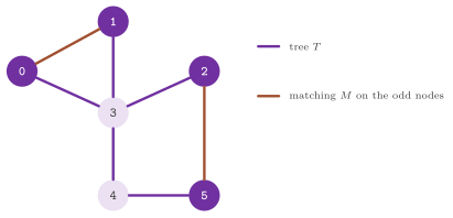
Finally, ChristofidesTsp< CM > implements the heuristic of Christofides
1976. It combines a minimum cost
spanning tree with a minimum cost perfect matching on the nodes of odd degree
of the tree (Figure 19.1), and it is the only class of the family with a
guaranteed approximation factor.
Algorithm 19.4 (Christofides).
1  T := minimum cost spanning tree of K_n                  (kruskal)
2  O := nodes of odd degree in T
3  M := minimum cost perfect matching of the complete graph on O
         (MaxWeightedPerfectMatching on the costs -c, on a SmartGraph)
4  H := the multigraph T + M on a SmartGraph
5  walk the Euler tour of H (EulerIt); append each node when first reached
In the code, the tree is computed by kruskal() (chapter
11), and the closed walk by EulerIt (chapter
18). The matching is computed by
MaxWeightedPerfectMatching (chapter 17) on a
SmartGraph with one node per node of \(O\) and with the negated costs as
weights; for this reason, the header warns that CM::Value must be a signed
number type. This graph has one edge for each pair of nodes of \(O\). Line 5
skips the nodes already visited, i.e., it shortcuts the closed walk as in
Lemma 19.2.
Lemma 19.4. For \(n\ge 3\), \(|O|\) is even and positive, the multigraph \(H\) of line 4 is connected with all degrees even, and line 5 produces a tour.
Proof. The sum of the degrees of \(T\) is \(2(n-1)\), and hence the number of the nodes of odd degree is even; it is positive, since a tree with at least two nodes has leaves. Then \(K_n\) restricted to \(O\) is complete with an even number of nodes and has a perfect matching \(M\), each node of \(O\) gains one edge of \(M\), and so every degree of \(H=T+M\) is even; \(H\) is connected since it contains \(T\). By Euler's theorem (chapter 18), \(H\) has a closed walk that uses each of its edges once, and this walk visits every node; listing the nodes at their first occurrence gives each node once, i.e., a tour. \(\square\)
Theorem 19.5. If \(c\) is metric and \(n\ge 3\), the tour returned by Algorithm 19.4 costs at most \(c(T)+c(M)\le\frac32 c^*\).
Proof. By Lemma 19.2, the tour costs at most the closed walk of line 5, i.e., \(c(T)+c(M)\). By Lemma 19.1, \(c(T)\le c^*\). Let \(H^*\) be an optimal tour, and let \(C_O\) be the cycle on \(O\) obtained from \(H^*\) by the shortcut of Lemma 19.2 (the nodes of \(O\) in the order of \(H^*\)), so that \(c(C_O)\le c^*\). Since \(|O|\) is even, the edges of \(C_O\) taken alternately form two perfect matchings \(M_1\) and \(M_2\) of \(O\) (equal to each other when \(|O|=2\)), with \(c(M_1)+c(M_2)=c(C_O)\le c^*\), and therefore \(c(M)\le\min\{c(M_1),c(M_2)\}\le c^*/2\). \(\square\)
Lemma 19.5. If \(c\) is metric and \(n\ge 3\), then \(c(M)\le c(T)\), and hence the tour of Algorithm 19.4 costs at most \(2c(T)\).
Proof. We show that \(T\) contains \(|O|/2\) edge-disjoint paths whose ends pair up the nodes of \(O\). Start from a node \(a\) of odd degree in the current set of edges, initially \(T\), and walk along edges not yet used; since \(T\) has no cycle, the walk is a path, and it can only stop at a node whose last edge it has just used, i.e., a node \(b\ne a\) of odd degree. Removing the edges of the path leaves the parity of the inner nodes unchanged and makes \(a\) and \(b\) even; repeating, one pairs all the nodes of \(O\). By the triangle inequality, the edge between the ends of each path costs at most the path, and these \(|O|/2\) edges form a perfect matching of \(O\) of cost at most \(c(T)\), since the paths are edge-disjoint and the costs are nonnegative. As \(M\) is a minimum cost perfect matching, \(c(M)\le c(T)\), and the second claim follows from the first part of the proof of Theorem 19.5. \(\square\)
Theorem 19.6. Algorithm 19.4 runs in \(O(n^3\log n)\) time, the bound of the header.
Proof. Line 1 runs Kruskal's algorithm on the \(n(n-1)/2\) edges in \(O(n^2\log n)\) time. Line 3 builds a graph with \(|O|\le n\) nodes and \(|O|(|O|-1)/2\) edges and runs on it the weighted perfect matching algorithm of chapter 17, whose \(O(nm\log n)\) bound gives \(O(n^3\log n)\). Lines 4 and 5 handle a multigraph of at most \(n-1+n/2\) edges in linear time. \(\square\)
In practice, the tours are usually much better than the bound of Theorem 19.5: in the example of §19.4 the tour costs less than 1.3 times the spanning tree.
abLEMON
In LEMON 1.3.1, the graph of the matching had two parallel edges for each
pair of nodes of \(O\), one per order of the pair, which doubled its edges
without changing the minimum cost of a perfect matching. The change is
not observable in the result beyond the choice among matchings of equal
cost; the test tsp_test checks the tours as before.
19.3 Improvement by 2-opt¶
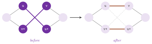
We now turn to Opt2Tsp< CM >, which implements the 2-opt local search of
Croes 1958. Given a tour, it looks
for two of its edges \(\{u,u^+\}\) and \(\{v,v^+\}\) that share no node, with
\(u^+\) and \(v^+\) the successors of \(u\) and \(v\), such that
and replaces them by \(\{u,v\}\) and \(\{u^+,v^+\}\) (a 2-opt move), which reverses the path from \(u^+\) to \(v\) (Figure 19.2). The search stops when no pair satisfies (19.3), i.e., at a 2-optimal tour.
There are three ways to give the starting tour. A call of run() starts from
the order of the node ids; run( path ) starts from a path structure, which
must be a valid path of \(n\) arcs (cf. checkPath() in chapter
8); and run( nodes ) starts from a
std::vector< Node > that holds all the nodes in the order of the tour. The
typical use is the improvement of the tour of a construction heuristic, e.g.,
by passing to run() the tourNodes() of an InsertionTsp. The tour is kept
as a list of two neighbors per node, without an orientation, which the private
iterator PathListIt follows by remembering the node it comes from; hence, a
move rewires four entries and costs \(O(1)\), with no explicit reversal of a
path.
Lemma 19.6. A 2-opt move turns a tour into a tour, whose cost is the old one minus the difference between the two sides of (19.3).
Proof. Removing the two edges, which share no node, splits the tour into the path from \(u^+\) to \(v\) and the path from \(v^+\) to \(u\), which together cover every node. The edge \(\{u,v\}\) joins the end \(v\) of the first to the end \(u\) of the second, and \(\{u^+,v^+\}\) joins their other ends, which closes a single cycle through all the nodes. The cost changes by \(c(u,v)+c(u^+,v^+)-c(u,u^+)-c(v,v^+)\). \(\square\)
Algorithm 19.5 (2-opt, first improvement).
1  restart:
2  for u := node 0, then along the tour, while u+ and u++ are not node 0:
3      for v := u++, then along the tour, while v is not node 0 and not
              the predecessor of u:
4          if (19.3) holds for (u, u+) and (v, v+):
5              replace {u,u+}, {v,v+} by {u,v}, {u+,v+}   (checkOpt2())
6              goto restart
7  list the tour from node 0 and recompute its cost
Theorem 19.7. Algorithm 19.5 terminates with a 2-optimal tour. A pass that finds no move evaluates (19.3) on each of the \(n(n-3)/2\) pairs of edges of the tour that share no node, and the whole run costs \(O(n^2(k+1))\) time, where \(k\) is the number of moves; for integer costs, \(k\le c(H_0)-c^*\), where \(H_0\) is the starting tour.
Proof. Let the tour be \(p_0=0,p_1,\dots,p_{n-1}\) in the order of the
iterators, and let the edge \(a\) be \(\{p_a,p_{a+1}\}\) (indices modulo \(n\)).
Line 2 takes \(u=p_a\) for \(a=0,\dots,n-3\), and line 3 takes \(v=p_b\) for
\(b=a+2,\dots,n-1\), except \(b=n-1\) when \(a=0\), since then \(v^+=p_0=u\). These
are exactly the pairs \(a<b\) of edges that share no node, \(n(n-3)/2\) in all.
Hence a pass ends at line 7 only if no such pair satisfies (19.3), i.e., the
tour is 2-optimal. By Lemma 19.6 each move gives a tour and, by (19.3),
decreases its cost strictly. For a floating-point Cost, the comparison is
made on the two computed sums, and since rounding is monotone, a computed sum
on the left larger than the one on the right implies the same inequality
between the exact sums, so that the exact cost of the tour (the sum of the
stored costs of its edges) still decreases strictly. No tour can therefore
occur twice, and the number of tours is finite; hence the algorithm
terminates. Each pass before a move costs at most the \(O(n^2)\) of a full pass,
and so does the last one. For integer costs each move decreases the cost by at
least 1, and no tour costs less than \(c^*\). \(\square\)
The number of moves is not polynomially bounded in general, even for points of the plane (Englert, Röglin and Vöcking 2014), and the header describes the method as rather slow but effective. Note that (19.3) is a strict comparison without tolerance; for floating-point costs, a move whose gain is below the rounding of the four costs may or may not be taken. For points of the plane, 2-optimality has a geometric meaning, which explains the quality of the tours in practice and gives the check of the example of §19.4.
Lemma 19.7. Let the nodes be points of the
plane, no three of them collinear, with the Euclidean distances as costs. (i)
If the segments of two edges \(\{u,u^+\}\) and \(\{v,v^+\}\) of a tour cross, they
satisfy (19.3), and therefore a 2-optimal tour has no crossing edges. (ii) If
the points are in convex position, the only tour without crossing edges is the
boundary of their convex hull, which is therefore both the optimal tour and
the tour returned by Opt2Tsp, whatever its starting tour.
Proof. (i) Let the two segments cross at the point \(x\). By the triangle
inequality of the plane, \(c(u,v)\le|ux|+|xv|\) and
\(c(u^+,v^+)\le|u^+x|+|xv^+|\), and both inequalities are strict, since \(x\) lies
on the segment from \(u\) to \(v\) only if \(u,x,v\), and hence \(u,u^+,v\), are
collinear. Summing, and since \(|ux|+|xu^+|=c(u,u^+)\) and
\(|vx|+|xv^+|=c(v,v^+)\), one obtains (19.3). (ii) Let \(\{p,q\}\) be an edge of a
tour that is not a side of the convex hull. The line through \(p\) and \(q\) then
leaves points on both of its sides, and the rest of the tour, a path from \(q\)
to \(p\) through all the other points, has an edge \(\{a,b\}\) with \(a\) and \(b\) on
opposite sides. In convex position, the segment \(ab\) meets the line inside the
convex hull, whose intersection with the line is the segment \(pq\); hence
\(\{a,b\}\) crosses \(\{p,q\}\). A tour without crossings therefore uses only
sides of the hull, i.e., it is its boundary. An optimal tour is 2-optimal,
since a move would decrease its cost, and so is the tour of Opt2Tsp (Theorem
19.7); by (i) neither has crossings, and both are the boundary. \(\square\)
19.4 Choosing a heuristic, and an example¶
We summarize the trade-off as the documentation of the group does. The fastest
methods are NearestNeighborTsp, GreedyTsp and InsertionTsp, and the
insertion is usually quite effective; ChristofidesTsp is somewhat slower,
but it has the best guarantee. Finally, Opt2Tsp is the slowest, it usually
gives the best tours in practice, and it can improve the tour of any other
method.
On random Euclidean instances, the farthest insertion followed by 2-opt is a sensible default. The run of the program described below on 40 points of the unit square illustrates this (on one instance, and therefore only as an illustration). The nearest neighbor and the greedy tours cost 5.58 and 5.33, the four insertion rules give 5.37 (nearest), 4.76 (farthest), 5.20 (cheapest) and 4.93 (random), and Christofides' tour costs 4.90, against 3.81 for the spanning tree. Also, 2-opt brings the farthest insertion tour to 4.76, and the other three to between 4.83 and 5.21.
The program manual/examples/19-tsp.cc (the test manual_19_tsp) checks
these properties on two instances. On twelve points of a circle, numbered out
of their angular order, it checks that every tour costs at least the perimeter
of the regular polygon. It also checks that Christofides' tour costs at most
\(3/2\) of it (Theorem 19.5), and that the 2-opt tour from the order of the ids
costs the perimeter (Lemma 19.7). On the 40 random points, it checks that each
tour visits each node once and costs the returned value, that it costs at
least the minimum spanning tree (Lemma 19.1), that Christofides' tour costs at
most twice the tree (Lemma 19.5), and that 2-opt does not worsen the tour it
starts from.
19.5 The maximum clique problem¶
Given an undirected graph \(G=(V,E)\), \(n=|V|\), a clique is a set \(C\subseteq V\) of pairwise adjacent nodes. In the maximum clique problem one looks for a clique of largest cardinality \(\omega(G)\), i.e.,
Since the problem is NP-hard and hard to approximate, the library offers two
algorithms with different aims. GrossoLocatelliPullanMc is a heuristic that
quickly finds a "large" clique, without a proof of its maximality.
TomitaSekiMc is an exact branch and bound that proves the clique it finds
maximum, in a time that may grow exponentially with the size of the graph,
unless a limit on its search tree stops it first. Both copy the graph into an
\(n\times n\) adjacency matrix of char, indexed by the order of the node
iterator, which costs \(O(n^2)\) memory and \(O(n^2+m)\) time before the search
starts, \(m\) being the number of edges. Both also ignore loops (a loop does not
make a node adjacent to itself) and parallel edges.
abLEMON
TomitaSekiMc is new in abLEMON (version 1.5.0). In LEMON 1.3.1,
GrossoLocatelliPullanMc ran forever on a graph with a loop, which made a
node adjacent to itself and kept it among the candidates of the clique it
already belonged to; abLEMON ignores loops when it builds the adjacency
matrix.
19.6 The iterated local search of Grosso, Locatelli and Pullan¶
Our heuristic class, GrossoLocatelliPullanMc< GR >, implements the iterated
local search of Grosso, Locatelli and Pullan
2008 on an undirected graph of type
GR. It keeps a current clique \(C\) and, for each node \(w\), the number
\(\delta(w)\) of nodes of \(C\) not adjacent to \(w\), where a node of \(C\) counts
itself (the matrix has no loops). Thus, \(\delta(w)=0\) holds for the nodes that
can be added to \(C\), and \(\delta(w)=1\), with \(w\notin C\), for the nodes that
can replace one node of \(C\). An iteration perturbs \(C\) and improves it by a
local search with a tabu set; the largest clique found over all the iterations
is the result.
Algorithm 19.6 (One iteration of start()).
1  restart := restart + 1
   R := { w : delta(w) >= 4 }; r := uniform in R, or in V if R is empty
2  remove from C the nodes not adjacent to r; add r to C          (restart)
3  tabu := {}; max_swap := |C|
4  while select < max_select:
5      select := select + 1
6      if a non-tabu w has delta(w) = 0: add w to C
           (and max_swap := |C| while tabu is still empty)
7      elif a non-tabu w not in C has delta(w) = 1:
           add w, remove the one node v of C not adjacent to w, tabu += v
           max_swap := max_swap - 1; leave the loop if max_swap <= 0
8      elif some w has delta(w) = 0 (tabu allowed): add w to C
9      else leave the loop
10 if |C| > |best|: best := C; return SIZE_LIMIT if |best| >= max_size
11 update the penalties of the rule
The iterations are repeated while select < max_select and restart <
max_restart, where max_restart, max_select and max_size are the three
limits described below; at the end, run() returns ITERATION_LIMIT if
restart has reached its limit, and STEP_LIMIT otherwise. The 4 of line 1
is a constant of the class (the restart based on \(\delta\) is always on), and
the update of \(\delta\) after each addition or removal is one pass over a row
of the matrix, in addCliqueNode() and delCliqueNode().
Lemma 19.8. At all times, \(C\) and best are
cliques of \(G\) and \(\delta(w)=|\{x\in C: x=w \text{ or } \{x,w\}\notin E\}|\)
for every node \(w\).
Proof. Initially \(C\) and best are empty and \(\delta=0\); every change of
\(C\) is made by addCliqueNode() and delCliqueNode(), which increase or
decrease by one the \(\delta\) of the nodes not adjacent to the node added or
removed, the node itself included, and this keeps the formula. Line 2 leaves
in \(C\) only nodes adjacent to \(r\) and then adds \(r\), so that \(C\) stays a
clique. Lines 6 and 8 add a node \(w\) with \(\delta(w)=0\), i.e., \(w\notin C\) and
adjacent to every node of \(C\). At line 7, \(w\notin C\) and \(\delta(w)=1\), so
that exactly one node \(v\) of \(C\) is not adjacent to \(w\), and \(C-v+w\) is a
clique. Finally, best is a copy of \(C\). \(\square\)
Theorem 19.8. Each iteration of Algorithm 19.6
performs at most \(2n\) steps, i.e., passes through line 5, and costs \(O(n^2)\)
time; hence run() performs at most \(\min\{I,\,S\}\) iterations, where \(I\) is
the iteration limit and \(S\) the step limit, and costs
\(O(n^2+m+n^2\min\{I,S\})\) time.
Proof. Each step but the last of the iteration performs a move. An addition
(lines 6 and 8) increases \(|C|\), and a swap (line 7) keeps it, so that there
are at most \(n-1\) additions after the restart, which leaves \(|C|\ge 1\). Before
the first swap, max_swap is at most \(|C|\le n\), and after it the tabu set is
no longer empty and max_swap is never reset; since each swap decreases it
and the loop is left when it reaches 0, there are at most \(n\) swaps. Adding
the last step, which leaves the loop or reaches the step limit, an iteration
has at most \(2n\) steps. Each step costs \(O(n)\), i.e., a scan of the nodes by
the rule and one or two passes over a row of the matrix, and so do lines 1, 2,
10 and 11. Each iteration increases restart by one and select by at least
one, which gives the bound on the iterations, and the initialization of
init() costs \(O(n^2+m)\). \(\square\)
Thus every run ends, although with both limits disabled the bound of Theorem
19.8 is the largest int, and the header warns that one should set a
reasonable limit on the iterations or on the steps. The node selected among
the eligible ones at lines 6, 7 and 8 depends on the rule passed to
run( rule ), of the enumeration SelectionRule, and each selection scans
the nodes in cyclic order from a starting index drawn uniformly at random.
With RANDOM it is the first eligible node in this order; with DEGREE_BASED
it is an eligible node of maximum degree, ties going to the first one in the
order; with PENALTY_BASED, the default, it is an eligible node of minimum
penalty, ties going to the first one, as in Grosso, Locatelli and Pullan
2008. The three rules are the
private classes RandomSelectionRule, DegreeBasedSelectionRule and
PenaltyBasedSelectionRule, of which start() is a template, and each of
them provides the three selections and the update() of line 11, empty for
the first two.
The penalties start at zero at each run() and are updated at line 11 as in
DLS-MC (Pullan and Hoos 2006).
Those of the nodes of the current clique increase by one, and every \(p_d\)
iterations all the positive ones decrease by one, where the penalty delay
\(p_d\) is set by penaltyDelay( pd ) (2 by default, and a value smaller than 1
is taken as 1). Larger values keep the nodes of the recent cliques out of the
next ones for longer, and the best value depends on the graph (DLS-MC uses
values from 1 to about 50). The smallest value makes the rule degenerate, as
follows.
Lemma 19.9. With \(p_d=1\), all the penalties
stay at zero, and run( PENALTY_BASED ) and run( RANDOM ), started with
generators in the same state, give the same clique and the same termination
cause.
Proof. With \(p_d=1\), every update first increases the penalties of the nodes
of \(C\) and then decreases every positive penalty; by induction on the updates,
the penalties are zero before each update, and hence also after it. With all
the penalties equal, the strict comparison of the rule selects the first
eligible node in the cyclic order, which is the node that RANDOM selects.
Both rules draw one random starting index per selection, in the same sequence
of calls, and the restarts draw from the same generator. By induction on the
steps, the two runs pass through the same states. \(\square\)
abLEMON
In LEMON 1.3.1 the penalties were never updated (the function update()
of the rule was empty), and PENALTY_BASED, the default rule, selected
the same node as RANDOM; penaltyDelay() is new. Also, the constructor
without a seed now uses the global generator rnd, as its documentation
says, where it copied it, so that two objects built one after the other
drew the same sequence.
Three limits control the search; each is set by a function that returns a
reference to the object, and read by the function of the same name without
argument. The function iterationLimit( int ) sets the number of iterations
max_restart, 1000 by default; stepLimit( int ) sets the number of steps
max_select over all the iterations, by default \(-1\); and sizeLimit( int )
sets the clique size max_size at which the search stops, by default \(-1\),
which stands for the number of nodes. A negative iteration or step limit means
no limit (the largest int), and with a limit of zero no iteration is made,
so that the clique is empty and the cause is ITERATION_LIMIT (or
STEP_LIMIT for a step limit of zero). The size limit is tested only when an
iteration has found a larger clique (line 10), and therefore a size limit of 0
stops the search after the first iteration. The function run( rule ) returns
the cause of the termination, of the enumeration TerminationCause:
ITERATION_LIMIT, STEP_LIMIT or SIZE_LIMIT. The last one is also the
answer on a graph with no node (clique of size 0) and on a graph with one node
(clique of size 1).
The random choices use a generator of type Random (chapter
8), which depends on the constructor.
GrossoLocatelliPullanMc( graph ) draws from the global generator rnd,
which it advances, so that two objects built one after the other draw
different sequences; GrossoLocatelliPullanMc( graph , seed ) draws from a
generator of its own seeded with seed, and
GrossoLocatelliPullanMc( graph , random ) from a copy of the given one.
Since the object may refer to a generator it owns, it cannot be copied (its
copy constructor and assignment are private). The results are read by
cliqueSize() and by cliqueMap( map ), which writes true on the nodes of
the clique and false elsewhere, in a writable node map with bool (or
convertible) values. Also, the iterator CliqueNodeIt, constructed from the
algorithm object, lists the nodes of the clique in the order of the node
iterator; it converts to Node, compares with INVALID, and its postfix
increment returns a Node, not an iterator.
19.7 The exact algorithm of Tomita and Seki¶
For the exact solution, TomitaSekiMc< GR > implements the branch and bound
MCQ of Tomita and Seki 2003 on an
undirected graph of type GR, exported as Graph. A node of its search tree
is a clique \(C\) together with the set \(P\) of the candidates, i.e., nodes
adjacent to all the nodes of \(C\). The bound that prunes the tree is the number
of colors of a proper coloring of the subgraph induced by \(P\), which no clique
of \(P\) can exceed.
Lemma 19.10. If the nodes of \(P\) are partitioned into \(k\) independent sets, a clique contained in \(P\) has at most \(k\) nodes; hence, no clique that extends \(C\) by nodes of \(P\) is larger than \(|C|+k\).
Proof. Two nodes of a clique are adjacent, and two nodes of an independent set are not; a clique therefore has at most one node in each of the \(k\) sets. \(\square\)
In colorSort(), the coloring is computed greedily: each candidate, in the
order of \(P\), goes into the first color class that contains none of its
neighbors, or into a new class. The candidates are then listed by color, in
the vector order, and color[k] is the number of the class of order[k].
Lemma 19.11. The classes of colorSort() are
independent sets, and the prefix order[0..k] is contained in the first
color[k] classes; hence, by Lemma 19.10, no clique extending \(C\) by nodes of
order[0..k] has more than \(|C|+\)color[k] nodes. The function costs
\(O(|P|^2)\) time.
Proof. A node enters a class only if it has no neighbor there, and the
classes are disjoint, so that each is an independent set. Since order lists
the classes in increasing order and color[k] is the class of order[k],
every node of the prefix belongs to a class of number at most color[k]. Each
candidate is compared with at most all the nodes already placed, i.e., with
\(O(|P|)\) nodes. \(\square\)
Algorithm 19.7 (Tomita and Seki,
expand( P )).
1  order, color := colorSort(P)
2  for k from |P| - 1 down to 0:
3      if |C| + color[k] <= |best|: return                    (Lemma 19.11)
4      if the tree limit is reached: stopped := true; return
5      count a node of the search tree; v := order[k]; C := C + v
6      P' := { order[j] : j < k, order[j] adjacent to v }
7      if P' is empty: best := C if |C| > |best|
8      else expand(P')
9      C := C - v; return if stopped
At the root, \(C\) is empty and the candidates are all the nodes, sorted by
nonincreasing degree as Tomita and Seki order them; the degree counts distinct
neighbors, the sort is stable, and ties keep the order of the node iterator.
The function treeLimit( long long ) sets the largest number of nodes of the
search tree, i.e., of the cliques that line 5 extends, after which run()
stops; a negative value, the default (\(-1\)), means no limit, and a limit of 0
stops the search before its first node.
Theorem 19.9. With no tree limit, run()
returns true and cliqueSize() is \(\omega(G)\). With a tree limit, the
clique found is a clique of \(G\), and if run() returns true it is maximum.
Proof. By induction on line 5, \(C\) is a clique and every node of \(P\) is
adjacent to all of \(C\), since \(P'\) keeps the candidates adjacent to \(v\); hence
best, a copy of \(C\), is a clique. We show by induction on \(|P|\) that, if
expand( P ) is not stopped, then on return best is at least as large as
every clique \(K\) with \(K\supseteq C\) and \(K\setminus C\subseteq P\). Let
\(v=\)order[k] be the node of \(K\setminus C\) of largest index (if \(K=C\), the
clique \(C+v\) of any \(v\in P\) is larger and is covered by what follows, since
expand() is called only with \(P\) not empty). The loop stops before reaching
\(k\) only at line 3 for some \(k'\ge k\), where
\(|K|\le|C|+\)color[k']\(\le|\)best\(|\) by Lemma 19.11, since \(K\setminus C\)
lies in order[0..k']. Otherwise the branch of \(v\) is entered,
\(K\setminus(C\cup\{v\})\subseteq P'\), and either \(P'\) is empty, in which case
\(K=C+v\) is recorded at line 7, or expand( P' ) covers \(K\) by the induction
hypothesis. Applying the claim at the root, with \(C=\emptyset\) and \(P=V\),
gives cliqueSize() \(=\omega(G)\) whenever the search is never stopped, and
run() returns true exactly in this case. \(\square\)
Theorem 19.10. The nodes of the search tree
are distinct cliques of \(G\), and hence their number treeSize() is at most
the number of nonempty cliques of \(G\), less than \(2^n\). The run costs
\(O(n^2+m)\) time before the search and \(O(n^2)\) time per node of the tree, with
\(O(n^2)\) memory.
Proof. A node of the tree is the clique \(C+v\) of line 5. Two nodes with the same clique \(K\) would branch on its last node in the order of the parent call, which shows by induction that they have the same parent call and the same \(v\), i.e., that they are the same node. Line 1 costs \(O(|P|^2)=O(n^2)\) by Lemma 19.11, and line 6 costs \(O(|P|)\) per iteration of the loop, i.e., \(O(n^2)\) per call. The matrix takes \(O(n^2)\) memory, and the recursion, of depth at most \(\omega(G)\), keeps \(O(n)\) integers per level. \(\square\)
In the worst case the time is exponential, as for any exact algorithm for
(19.4) known so far, and the size of the tree depends strongly on the density
of the graph. The function run() returns true when the clique found is
proved maximum, and false when the limit stopped the search first; in this
case the clique is the largest one found so far. The results are read by
cliqueSize(), by treeSize() (the number of nodes of the search tree of the
last run) and by cliqueMap( map ), with the same contract as in
§19.6. On sparse graphs the coloring bound prunes
almost all the branches: in the program described below, a planted clique of 9
nodes in a random graph of 60 nodes and density 0.2 is proved maximum with a
search tree of 9 nodes. On dense random graphs of a few hundred nodes,
instead, the tree may already be very large.
The program manual/examples/19-clique.cc (the test manual_19_clique)
compares the exact algorithm with the enumeration of all the subsets on five
random graphs of 14 nodes. On the graph with the planted clique, it checks
that the heuristic, seeded and stopped at the maximum size, finds a clique no
larger than the maximum one, and that the rules RANDOM and PENALTY_BASED
with the same seed give the same clique when the penalty delay is 1 (Lemma
19.9); finally, it stops an exact search after 5 nodes of its tree.
19.8 Exercises¶
Exercise 19.1. Check on random Euclidean
instances that each tour returned by the five TSP classes costs at least the
minimum spanning tree (Lemma 19.1), and that the tour of ChristofidesTsp
costs at most twice it (Lemma 19.5); manual/examples/19-tsp.cc does it for
40 points.
Exercise 19.2. Give five points of the plane,
not in convex position, and a 2-optimal tour on them that is not optimal;
deduce that Lemma 19.7 (ii) needs the convex position, and check it with
Opt2Tsp::run( nodes ) started from that tour (manual/examples/19-tsp.cc
checks the convex case on twelve points of a circle).
Exercise 19.3. Build a metric instance on which
NearestNeighborTsp returns a tour much more expensive than InsertionTsp
with the FARTHEST rule, e.g., points on a line with exponentially growing
gaps, and measure the ratio as \(n\) grows.
Exercise 19.4. Give a non-metric instance on
which the shortcuts of Algorithm 19.4 increase the cost of the Euler tour, and
compare the resulting tour with the bound of Theorem 19.5 (test/tsp_test.cc
checks only metric instances).
Exercise 19.5. Count the evaluations of (19.3)
made by Opt2Tsp from the order of the node ids and from the tour of
InsertionTsp, on random Euclidean instances of growing size, and relate them
to the \(n(n-3)/2\) evaluations of a pass (Theorem 19.7).
Exercise 19.6. Verify on random graphs that
TomitaSekiMc finds a clique of the size given by the enumeration of all the
subsets, and that a tree limit of 1 stops the search after one node
(test/tomita_seki_mc_test.cc and manual/examples/19-clique.cc).
Exercise 19.7. Run GrossoLocatelliPullanMc
with the rules RANDOM and PENALTY_BASED and the same seed on the same
graph, observe that they return the same clique when the penalty delay is 1
(Lemma 19.9); then compare the sizes of the cliques found by PENALTY_BASED
with penalty delays from 2 to 50 (manual/examples/19-clique.cc checks the
first part; test/max_clique_test.cc checks the termination causes of the
three rules).
Exercise 19.8. Plot the size of the search tree
of TomitaSekiMc (treeSize()) on random graphs of 100 nodes as the density
grows from 0.1 to 0.9, and find where the coloring bound stops being
effective.