14. Certificates and the k best flows
We now turn to what the library gives besides one optimal flow. When a minimum
cost flow problem has no optimal flow, the four algorithms of chapter
13 give a certificate of the answer, i.e., a set
of nodes that proves it infeasible or a cycle that proves it unbounded, which
a program can check on the data; they can also give several such certificates,
in a definite order. When the problem has an optimal flow, the class
KBestFlows of lemon/k_best_flows.h gives the \(k\) integer flows of least
cost, and the class KBestExtremeFlows of lemon/k_best_extreme_flows.h
gives the \(k\) vertices of least cost of the polyhedron of the flows, together
with distinct optimal potentials. Section 14.1 treats the certificates of
infeasibility and section 14.2 those of unboundedness, both implemented in
lemon/bits/mcf_certificate.h; sections 14.3 and 14.4 describe the two
classes of the \(k\) best flows, and section 14.5 the alternative optimal
potentials. We keep the notation of section
13.1, i.e., the GEQ form (13.1), the reduced
costs (13.3), the optimality conditions (13.5) and the residual network of a
flow, and, as there, we state the results in exact arithmetic.
abLEMON
The content of this chapter is new with respect to LEMON 1.3.1, which gave
no certificate and no other flow than an optimal one: infeasibleCut()
and unboundedCycle() appeared in version 1.6.0, infeasibleCuts(),
disjointInfeasibleCuts(), unboundedCycles(), KBestFlows and
KBestExtremeFlows in version 1.7.0, the alternative optimal potentials
in version 1.8.0, and their method PIVOTS, the cuts of NetworkSimplex
taken from its last tree, the ties of infeasibleCuts() and the single
run of Howard's algorithm in unboundedCycles() in version 1.9.0.
14.1 Certificates of infeasibility
14.1.1 Violated sets
For a set \(N'\subseteq V\) of nodes, the violation of \(N'\) under GEQ is its supply less what can leave it,
where no arc out of \(N'\) may have an infinite upper bound (such a set proves no infeasibility). Under LEQ the same holds with \(-sup\) in place of \(sup\) and the arcs taken backwards, i.e., the demand of \(N'\) less what can enter it. A set of positive violation proves (13.1) infeasible, since its supply cannot leave it, and the converse holds too. As in section 12.4, let \(sup'\) be the supplies net of the lower bounds and \(P\) the sum of their positive values. Let also \(N\) be the network that joins a source \(\sigma\) to each node \(u\) with \(sup'(u)>0\) by an arc of capacity \(sup'(u)\), each node \(u\) with \(sup'(u)<0\) to a target \(\tau\) by an arc of capacity \(-sup'(u)\), and that gives each arc \(uv\) the capacity \(upper(uv)-lower(uv)\).
Theorem 14.1. (Gale, Hoffman.) Problem (13.1) is infeasible if and only if some set \(N'\) has \(viol(N')>0\). For each cut \(\{\sigma\}\cup N'\) of \(N\), \(viol(N')=P-cap(\{\sigma\}\cup N')\); hence, the largest violation is \(P\) less the value of a maximum flow of \(N\), and the source side of each minimum cut, without \(\sigma\), is a set of largest violation.
Proof. The constraints of (13.1) are those of (12.5), and (14.1) is the right-hand side less the left-hand side of (12.6). The first statement is therefore Theorem 12.5, and the identity is (12.7). By Theorem 12.1, the smallest capacity of a cut of \(N\) is the value of a maximum flow, which gives the rest. \(\square\)
This is the feasibility theorem of Gale 1957 and Hoffman 1960. Under LEQ the same holds on the reversed network with the negated supplies.
14.1.2 The interface
After a run() that returned INFEASIBLE, the four classes give three kinds
of certificates, as sets of nodes of the digraph (vectors of Node); after
any other answer they are empty.
infeasibleCut()returns one set \(N'\) with \(viol(N')>0\).infeasibleCuts( k )returns the \(k\) sets of largest violation, in the order of their violations, at most \(k\) and only those that prove the problem infeasible.disjointInfeasibleCuts()returns sets of positive violation that are pairwise disjoint, with no arc between any two of them.
Each set is checked on the data, by (14.1), before it is returned. In floating
point the check requires the violation to exceed both the tolerance on the
flows and the round-off of the sum, i.e., the default epsilon of Tolerance
times one plus the sum of the absolute values of the terms of (14.1); when it
does not, no set is returned. Hence, a set that only round-off makes violated
is never given as a certificate. NetworkSimplex gives its sets under the
supply type, i.e., by (14.1) with the arcs reversed and the supplies negated
under LEQ, and the other three classes use the GEQ form. In all of them the
sets are computed and checked on the data as they are when the function is
called, which must therefore be those of the last run() (the supply type
included).
If it proves the answer, the set of infeasibleCut() is the one that the
algorithm has at hand when it finds no feasible flow, at no further cost. It
is the set of all the nodes when the supplies sum to the wrong sign (positive
under GEQ, negative under LEQ). Otherwise, it depends on the class, as
follows.
NetworkSimplextakes it from its last tree. By the proof of Theorem 13.3, the tree potentials \(y\) under the costs of the first phase (one on the artificial arcs that should carry no flow, zero on the others) are an optimal solution of the dual of the first phase; so is the indicator of each level set of them, i.e., of the nodes whose potential is at least, or at most, a value, and the first level set that proves the answer is kept.CostScalingandCycleCancelingtake the nodes above the level that the push-relabel algorithm of their starting flow leaves empty, together with the node it was lifting, from which no residual arc leaves (section 13.5); by Theorem 12.6 this set has a positive violation.CapacityScalingtakes the nodes, other than the root, that its last search for a shortest augmenting path reached from a node with excess without finding a deficit; by the proof of Theorem 13.7, no residual arc leaves this set, and it has a positive violation.
If that set does not prove the answer (which may happen, although rarely, in
floating point), the class falls back on a set of largest violation, by one
maximum flow of Preflow on the network of Theorem 14.1. Thus,
infeasibleCut() costs nothing beyond the run in exact arithmetic, and one
maximum flow at most; we remark that one can therefore call it without concern
even on "large" problems.
In turn, the sets of disjointInfeasibleCuts() are the weakly connected
components of the set of infeasibleCut() whose violation is positive, in the
order of their violations. Since no arc joins two components, the violation of
the set is the sum of those of its components; hence, the violations of the
sets given sum to at least that of the set. Note that they depend on the set
that the class has at hand: in the example of section 14.1.4, NetworkSimplex
gives a set of violation 4, whose two components are violated, while the other
three classes give a set of violation 2, which is a single component.
14.1.3 The k most violated sets
We find the sets of infeasibleCuts( k ) by the partition of Lawler
1972, applied to the cuts of the network
of Theorem 14.1 as in Hamacher, Picard and Queyranne
1984. Here the space of the sets
is split into parts, in each of which some nodes are fixed in the set and
some out of it. The best set of a part is found by a maximum flow in which a
node fixed in the set is joined to the source, and a node fixed out of it to
the target, by an extra capacity of \(2P+3\), which no minimum cut may contain.
Its violation bounds from above those of all the sets of the part. Once the
best set of a part is given, the part is split by its free nodes
\(u_1,u_2,\ldots\) in turn: the \(j\)-th child keeps \(u_1,\ldots,u_{j-1}\) as they
are in the set, and takes \(u_j\) out of the set if the set has it, in
otherwise.
Algorithm 14.1 (The k most violated sets).
1  root part: no node fixed; solve it by one maximum flow (Theorem 14.1)
2  give the sets that tie for the largest violation, from the residual
   digraph of that flow (the closed sets, Lemma 14.1), up to k of them
3  while fewer than k sets are given:
4      p := the part of largest bound (its own violation, or that of its
           parent if it is not solved yet; a solved part first on ties)
5      if p is not solved: solve it, from the maximum flow of its parent;
           if its best set violates a fix or is not violated, drop p;
           continue
6      give the best set of p unless it was already given; remove p
7      for each free node u_j of p, j = 1, 2, ...:
8          add the child that fixes u_1 .. u_{j-1} as in the set of p and
           u_j opposite to it, with the bound of p, not solved
Two devices keep the number of maximum flows rather small. First, a child
waits in the list with the violation of its parent as a bound, and its best
set is computed only when it is the most promising part; hence, a maximum flow
is made only for the parts that might hold one of the \(k\) sets, rather than
for each child of each set given. Second, the maximum flow of a part is a
preflow of each of its children, whose capacities are only larger (one more
fixed node adds capacity on one arc from the source or to the target); hence,
Preflow::init( flowMap ) starts each child from the flow of its parent
(chapter 12). The ties of step 2 come from Lemma 12.1,
as Picard and Queyranne 1980
observed; the partition then runs as usual, and a set that it finds again is
not given twice.
Lemma 14.1. (Closed sets.) Let \(x\) be a
maximum flow of \(N\). The minimum cuts of \(N\) are the sets that contain
\(\sigma\), do not contain \(\tau\), and are closed in the residual digraph of
\(x\), i.e., the unions of the closure of \(\sigma\) with the closures of strongly
connected components of that digraph that do not reach \(\tau\). The function
closedSets() lists them breadth first, from the closure of \(\sigma\), by
adding the closure of one component at a time.
Proof. The first statement is Lemma 12.1. The closure of a node (the set of the nodes it reaches) is closed, and so is a union of closed sets; conversely, a closed set contains the closure of each of its nodes, and hence equals the union of the closures of its components. A closed set holds \(\tau\) if and only if one of its components reaches \(\tau\), which the function excludes. \(\square\)
Lemma 14.2. A part that contains a set of positive violation has, as its best set, a minimum cut that respects its fixes, and that set has the largest violation in the part; a part whose minimum cut violates a fix contains no set of positive violation.
Proof. A cut \(\{\sigma\}\cup N'\) that respects the fixes cuts none of the extra capacities, and its capacity is \(P-viol(N')\) by Theorem 14.1; it is below \(P\) if \(viol(N')>0\). A cut that violates a fix cuts an extra capacity of \(2P+3>P\), and so does not attain the minimum when some set of the part has a positive violation. The same holds for the arcs of infinite capacity, which the network replaces by \(P+1\): a cut that contains one has a capacity above \(P\). \(\square\)
Theorem 14.2. (The k most violated sets.)
infeasibleCuts( k ) returns the \(\min\{k,q\}\) sets of largest violation,
where \(q\) is the number of sets of positive violation, distinct and in a
nonincreasing order of violation. It makes at most \(1+n\,s\) maximum flows,
where \(s\) is the number of parts whose best set was given; i.e., at most \(n\)
maximum flows for each set, as the header states.
Proof. We show by induction that the parts in the list partition the sets of positive violation not yet given (the ties of step 2 aside, which are the sets of largest violation by Lemma 14.1 and are given first). This holds for the root part. When a part \(p\) with best set \(S\) is removed, its children are pairwise disjoint (the \(j\)-th one differs from the earlier ones on \(u_j\)), and they are contained in \(p\). A set of \(p\) other than \(S\) differs from \(S\) on some free node, the first of which places it in exactly one child; hence, the children partition \(p\setminus\{S\}\). A dropped part contains no set of positive violation by Lemma 14.2. The bound of each part is at least the largest violation of its sets, since a child's sets are sets of its parent. Hence, when the part of largest bound is solved and its best set is violated, that set has a violation at least that of every set left, and the sets are given in a nonincreasing order. Each part is solved at most once, and each part whose best set is given adds at most \(n\) children, which proves the count. \(\square\)
14.1.4 An example
Figure 14.1 shows a problem of five nodes, in which the node \(a\) must send 4
units on an arc of capacity 2, and \(d\) must send 3 units on one of capacity 1,
while \(b\), with no supply, can only feed \(a\). The sets \(\{a\}\), \(\{a,b\}\) and
\(\{d\}\) have violation 2, and the sets \(\{a,d\}\) and \(\{a,b,d\}\) have
violation 4, the largest; hence, the four best sets of infeasibleCuts( 4 )
have the violations 4, 4, 2 and 2.
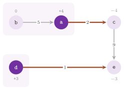
The program manual/examples/14-certificates.cc (the test
manual_14_certificates) solves the problem of Figure 14.1, and the unbounded
problem of section 14.2, with the four classes, and it checks each certificate
on the data. For infeasibleCuts() it checks positive violations (14.1) in a
nonincreasing order and distinct sets, and for disjointInfeasibleCuts()
pairwise disjoint sets with no arc between them; in the unbounded case it
checks closed cycles of negative cost made of arcs of infinite capacity,
pairwise arc-disjoint.
14.2 Certificates of unboundedness
A run returns UNBOUNDED only on a feasible problem with a directed cycle
whose arcs have infinite upper bounds and whose cost is negative; along such a
cycle the flow may grow without limit while the cost decreases (section
13.1). After such a run the four classes give
two kinds of certificates, both empty after any other answer.
unboundedCycle()returns one such cycle, as the vector of its arcs in the direction of the flow.unboundedCycles( k )returns at most \(k\) such cycles, pairwise arc-disjoint, in the order of their mean costs.
In NetworkSimplex the cycle is the one of the pivot that it could not
perform, i.e., its entering arc and the path of the tree between the two ends
of it, unless that path goes through an artificial arc, which by the proof of
Theorem 13.3 does not happen in exact arithmetic when \(M>nK\). In that case,
and always in the other three classes, the cycle is found by the algorithm of
Bellman and Ford on the arcs of infinite upper bound, run from a virtual node
joined to all the others. After each round the graph of the predecessors is
searched for a cycle, which is then returned (Lemma 14.3), and the search
gives up, returning no cycle, after \(4n+4\) rounds or when a round improves no
distance. In floating point the cycle is returned only if its cost is negative
beyond the round-off.
Lemma 14.3. (Tarjan.) If the graph of the predecessors of the algorithm of Bellman and Ford contains a cycle, the cost of that cycle is negative.
Proof. Let \(C\) be the cycle, and consider the moment just before the last of its arcs, \(p(v)v\), was set, by a strict improvement \(d(v)>d(p(v))+c(p(v)v)\). For each other arc \(p(w)w\) of \(C\), \(d(w)\) was set to \(d(p(w))+c(p(w)w)\) when the arc was set, and \(d(p(w))\) can only have decreased since; hence, \(d(w)\geq d(p(w))+c(p(w)w)\). Summing over the arcs of \(C\), in which each node appears once as a head and once as a tail, the distances cancel, and \(0>\sum_{a\in C}c(a)\). \(\square\)
One might think of the cycle of least total cost as the natural choice for
several cycles, but it is NP-hard to find, since it would decide whether a
digraph is Hamiltonian (cf. Exercise 14.3). Instead, the cycles of
unboundedCycles( k ) are those of minimum mean cost, which are the most
negative per arc. Howard's algorithm (class HowardMmc, chapter
16), run on the arcs of infinite upper bound,
ends on each strongly connected component with a policy whose cycle has the
minimum mean of the component (Dasdan
2004); the class gives these
cycles through componentCycleNum() and componentCycle().
Algorithm 14.2 (Arc-disjoint negative cycles).
1  C := empty; T := the arcs of infinite upper bound
2  while |C| < k and T is not empty:
3      run Howard's algorithm on the arcs of T
4      for each strongly connected component, take its cycle of minimum
       mean if that mean is negative beyond the round-off
5      if none: stop
6      add them to C by increasing mean, up to k; remove their arcs from T
7  sort C by mean; return C
Lemma 14.4. The cycles of Algorithm 14.2 are pairwise arc-disjoint, each of negative cost, and the first one has the minimum mean of all the cycles of infinite upper bound.
Proof. The cycles of one run lie in distinct strongly connected components, and are therefore node-disjoint, and those of later runs use only the arcs not yet taken. The minimum cycle mean of a digraph is the least of those of its components, and the first run is made on all the arcs of infinite upper bound. A negative mean means a negative cost. \(\square\)
A cycle of a later run may have a smaller mean than some of an earlier one (never than the first one), which is why step 7 sorts them. Since one run of Howard's algorithm gives the cycles of all the components, the algorithm runs again only when fewer than \(k\) cycles were found.
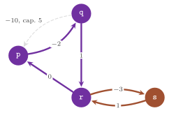
In the problem of Figure 14.2, the four nodes form one strongly connected
component of the arcs of infinite capacity, whose cycle of minimum mean is
\((r,s,r)\), of cost \(-2\) and mean \(-1\). A second run on the arcs left finds
\((p,q,r,p)\), of cost \(-1\) and mean \(-1/3\), and unboundedCycles( 3 ) gives
these two cycles, as the program of section 14.1.4 checks. The arc \((q,p)\)
closes with \((p,q)\) a cycle of cost \(-12\), but its capacity is finite; hence,
it bounds the flow on that cycle, and it never appears in a certificate.
14.3 The k best integer flows: KBestFlows
14.3.1 The algorithm
We now describe the class KBestFlows, which finds the \(k\) integer flows of
least cost of (13.1), in the order of their costs: first an optimal flow, then
the other optimal flows, if any, and then the suboptimal ones. The constraints
are brought to the equality form by an extra node, the root, with an arc of no
cost and no upper bound into each node, whose flow is the slack
\(N_f(u)-sup(u)\) of the node (i.e., the unmet demand). Its algorithm is the one
of Hamacher 1995, which rests on
the following property of the integer flows.
Theorem 14.3. (Hamacher.) Let \(f\) be a flow of least cost in a set of integer flows defined by integer bounds on the arcs. Then a second best flow of the set, if there is one, is obtained from \(f\) by sending one unit along a cycle of least cost of the residual network of \(f\), where an arc together with its own reverse does not count as a cycle.
Proof. Let \(g\) be a second best flow, i.e., one of least cost among the flows of the set other than \(f\). The difference \(g-f\) is an integer circulation that, on each arc, goes forward only where \(g>f\) and backward only where \(g<f\). It decomposes into unit cycles \(C_1,\ldots,C_p\) of the residual network of \(f\), each conformal to it; hence, no cycle uses an arc and its own reverse, and \(f+\chi(C_j)\) is a flow of the set for each \(j\), \(\chi\) denoting the unit flow along the cycle. Each \(C_j\) has a nonnegative cost, since \(f\) is a best flow, and \(f+\chi(C_j)\neq f\), so that its cost is at least that of \(g\). Hence, \(cost(g)=cost(f)+\sum_j cost(C_j)\geq cost(f)+cost(C_1)=cost(f+\chi(C_1))\geq cost(g)\), and \(f+\chi(C_1)\) is a second best flow; a cycle of least cost costs at most \(cost(C_1)\), and one unit along it gives a flow of the set different from \(f\). \(\square\)
Then the set of all the integer flows is split as in the partition of Lawler 1972, on an arc where the best flow and the second best flow differ, i.e., the arc \(a\) of the first residual arc of the cycle. On one side the flow of \(a\) stays on the side of its value in the best flow, which remains the best of that side; on the other it lies on the side of the value of the second best flow, which becomes the best of that side. Hence, the next flow of the sequence is the cheapest of the second best flows of the sides.
Algorithm 14.3 (K best integer flows).
1  f_1 := an optimal flow (NetworkSimplex, or initFlow()); if none: return
2  S := { (bounds of the problem, f_1) }; compute the second best of it
3  for i = 2, ..., k:
4      (B, f) := the set of S whose second best flow g is the cheapest;
       if no set has one: stop
5      f_i := g; let a be the arc of the first residual arc of the cycle
6      if g(a) > f(a): B' := B with lower(a) := f(a) + 1;
                       B  := B with upper(a) := f(a)
       else:           B' := B with upper(a) := f(a) - 1;
                       B  := B with lower(a) := f(a)
7      add (B', g) to S; compute the second best flows of (B, f), (B', g)
Theorem 14.4. (KBestFlows.) run( k ) gives
the \(\min\{k,q\}\) integer flows of least cost of (13.1) in a nondecreasing
order of cost, where \(q\) is the number of integer flows, provided that the
first flow is optimal.
Proof. We show by induction that the sets of \(S\) partition the integer flows not yet given, and that the given flow of each set is its best flow. This holds at the start. When the set \(B\) with best flow \(f\) and second best flow \(g\) is split, \(B\) (with the new bound on \(a\)) and \(B'\) are disjoint and their union is \(B\), since the flow of \(a\) is an integer. Also, \(f\) stays in \(B\) and is still its best flow, while \(g\) is in \(B'\) and is its best flow, since \(B'\subseteq B\setminus\{f\}\) and \(g\) is a best flow of \(B\setminus\{f\}\) by Theorem 14.3. The flows not yet given are those of the sets other than their best flows, and the cheapest of them is the cheapest of the second best flows. Hence, each flow given is a cheapest one among those not yet given. \(\square\)
In secondBest(), the second best flow of a set is found as follows. First,
potentials of the residual network of the best flow of the set are computed by
the algorithm of Bellman and Ford, from a virtual node joined to all the
others; since the best flow of the set leaves no cycle of negative cost, the
reduced costs are nonnegative (Theorem 13.2). Then, for each node \(v\), the
algorithm of Dijkstra computes the shortest paths from \(v\) on the reduced
costs, and for each residual arc \((u,v)\) the cycle of least cost through it is
the arc and a shortest path from \(v\) back to \(u\). A shortest path from \(v\) to
\(u\) is simple, so that the cycle is simple and contains the reverse of \((u,v)\)
only if the path is that reverse and nothing else; then one more search is
made without the reverse arc. Hence, as stated in the header, the \(k\)-th flow
takes \(O(nm\log n)\) time after the \((k-1)\)-th when few such searches are made,
and \(O(m^2\log n)\) at worst, with one search for each residual arc. Of course,
the sequence does not depend on the algorithm that found the first flow, but
for the order of the flows of equal cost.
14.3.2 The interface
KBestFlows< GR , V , C > takes the type of the digraph, the number type V
of the flows, of the bounds and of the supplies (by default int), and the
number type C of the costs (by default V), which it names Digraph,
Value and Cost. Its constructor takes the digraph, whose nodes and arcs it
numbers at once; the digraph must not change afterwards. Until they are given,
the bounds are 0 and infinite, the costs 1 and the supplies 0. Its setters,
each returning the object, are the following ones.
lowerMap( map ),upperMap( map ),costMap( map )andsupplyMap( map )copy the data as in chapter 13, an upper bound that is infinite or the largest value ofValuemeaning no bound.initFlow( map )gives an optimal flow to start from, which must be optimal for the data given, and after which no minimum cost flow algorithm is run.tolerances( flow , cost )sets the tolerances of section 13.3, which are given to theNetworkSimplexthat finds the optimal flow, a negative value leaving them to the data;flowTolerance()andcostTolerance()return those in use, as aTolerance< Value >and aTolerance< Cost >.
Then run( k ) finds the flows and returns their number, which is less than
\(k\) if the problem has fewer integer flows, and zero if \(k\leq 0\) or the
problem has no optimal flow (it is infeasible or unbounded). Its queries are
flowNum(), the number of flows of the last run, totalCost( i ),
flow( i , arc ) and flowMap( i , map ), for the \(i\)-th flow, where the
first one is the flow 0. Both the bounds and the supplies must be integer,
also with a floating-point V (whose values are then integer ones), since the
flows differ from each other by whole units. Also, an infinite upper bound is
allowed only if no cycle of negative cost is made of arcs of infinite upper
bound, or the problem has no optimal flow. We remark that the comparisons of
the search for the second best flows are exact on such data.
14.4 The k best extreme flows: KBestExtremeFlows
14.4.1 Vertices, bases and the ranking of Murty
Next, the class KBestExtremeFlows finds the \(k\) vertices of least cost of
the polyhedron of the flows of (13.1), in the order of their costs: first an
optimal vertex, then the other optimal ones, if any, and then those whose cost
exceeds the optimum by at most a given gap. As the header remarks, these are
the flows that a Lagrangian or a Benders decomposition may want several of,
since each vertex gives a different (sub)gradient, while a flow inside a face
gives a convex combination of those of its vertices. The class works, as
KBestFlows, on the network with the root and its arcs into the nodes, in the
equality form. A flow is a vertex if and only if the arcs strictly within
their bounds (the free arcs) form a forest (Lemma 14.5); a basis of a
vertex is a spanning tree that contains its free arcs, the other arcs being at
a bound. A vertex is degenerate when it has more than one basis, i.e., when
its free arcs do not span the nodes.
Lemma 14.5. A feasible flow is a vertex of the polyhedron of the flows if and only if its free arcs form a forest.
Proof. If the free arcs contain a cycle, sending a small amount \(\pm\delta\) around it gives two feasible flows whose midpoint is the flow, which is then no vertex. If they form a forest, fixing every other arc at its bound leaves a system of conservation equations on the arcs of a forest, which has at most one solution (a leaf of the forest determines the flow of its arc, and so on). Hence, the flow is the only feasible flow on which those bounds are tight, i.e., a vertex. \(\square\)
Its algorithm is the ranking of the extreme points of Murty 1968, which rests on the fact that the next vertex in the order of cost is adjacent to one of the vertices already given. Adjacency means here one pivot of the network simplex method away from one of their bases, i.e., along the cycle that a nonbasic arc closes with the tree, saturated. Candidates wait in a priority queue by their costs, and the bases of a degenerate vertex, which the pivots of zero amount reach, are all expanded.
Algorithm 14.4 (Ranking of the vertices).
1  x_1 := an optimal flow, made a vertex; T_1 := a basis of it
2  Q := { (cost(x_1), the basis T_1) }
3  while Q is not empty and fewer than k vertices are given:
4      take from Q the candidate of least cost; stop if beyond the gap
5      make its basis (one pivot from the expanded basis it came from)
6      skip it if the basis was already expanded
7      if basisLimit() bases were expanded: exact := false; stop
8      give its vertex if it is new
9      if its vertex already used up vertexBasisLimit(): exact := false;
       skip it
10     for each nonbasic residual arc r of the basis:
11         c := the cost after the pivot of r (if its cycle is bounded)
12         put (c, r) in Q unless c exceeds the gap (the degenerate pivots
           only if the vertex has not used up its limit)
13 if not exact: sort the vertices given by cost
A candidate is kept in the queue only as its cost, with the index of the
expanded basis and of the arc of its pivot; the basis it leads to is made only
when it leaves the queue. Thus, the memory is \(O(n+m)\) for each basis
expanded. Each pivot takes \(O(n)\) time for its cycle, and each basis
\(O(n(n+m))\) for all its pivots, as the documentation of basisLimit() puts
it.
As in KBestFlows, the first vertex is the optimal flow that NetworkSimplex
finds, or the one given by initFlow(), which need not be a vertex. It is
made a vertex by purify(): while the free arcs close a cycle, the cycle is
saturated in a direction in which it is bounded, the direction in which the
cost does not grow being tried first.
Lemma 14.6. purify() ends after at most
\(n+m\) saturations with a vertex whose cost is not larger than that of the flow
it started from, and equal to it if that flow is optimal.
Proof. A cycle of free arcs is bounded in at least one direction, since in each direction the arcs traversed backward have a finite residual capacity, and all the arcs traversed forward in one direction are traversed backward in the other. Saturating it leaves the other arcs as they are and takes at least one of its arcs to a bound, so that the number of free arcs decreases; at the end the free arcs form a forest, and the flow is a vertex by Lemma 14.5. The direction in which the cost does not grow is bounded unless the cycle is one of infinite capacity and negative cost, which a feasible problem with an optimal flow does not have, or of zero cost, in which case the other direction costs nothing either. At an optimal flow the free arcs have a zero reduced cost by (13.5), so that a cycle of them costs zero. \(\square\)
Lemma 14.7. At a nondegenerate vertex \(x\) with basis \(T\), the edges of the polyhedron at \(x\) are the directions of the cycles that the nonbasic arcs close with \(T\), each in the direction allowed by the bound of its arc, and the adjacent vertices are the vertices reached by saturating those of them that are bounded.
Proof. Every arc of \(T\) is free at \(x\). A direction \(d\) is feasible at \(x\) if and only if it is a circulation that moves each nonbasic arc only away from its bound. Such a circulation is determined by its values on the nonbasic arcs (the tree arcs follow), and it is therefore the nonnegative combination \(\sum_e d(e)\,\chi(C_e)\) of the cycles \(C_e\), oriented as allowed, with coefficients the moves of the nonbasic arcs. These cycles are linearly independent, each containing a nonbasic arc that the others do not; hence, the cone of the feasible directions is simplicial, and its extreme rays, the edges at \(x\), are the directions \(\chi(C_e)\). Moving along a bounded one up to the first bound reached gives the adjacent vertex. \(\square\)
Theorem 14.5. (Murty.) Suppose that the vertices that Algorithm 14.4 expands are nondegenerate and that no limit acts. Then it gives the vertices of the polyhedron of the flows, up to \(k\) and within the gap, in a nondecreasing order of cost, the first one optimal.
Proof. Let \(X\) be the set of the vertices given so far, which contains an optimal one, and let \(w\) be a vertex of least cost among those not in \(X\). If some edge at \(w\) leads to a vertex of smaller cost, that vertex is in \(X\) (by the choice of \(w\)), and \(w\) is adjacent to \(X\). Otherwise no edge at \(w\) decreases the cost, and no unbounded edge does either, since the problem has an optimal flow; as the cone of the feasible directions at \(w\) is generated by its edges, \(w\) is optimal. The optimal vertices are those of the optimal face, whose graph of vertices and edges is connected; since \(X\) contains an optimal vertex, some optimal vertex outside \(X\) is adjacent to an optimal vertex of \(X\), and its cost is that of \(w\). In both cases the cheapest vertex adjacent to \(X\) and outside \(X\) has the cost of \(w\), and by Lemma 14.7 it is among the candidates of the queue, which gives the next vertex in the order of cost. \(\square\)
We remark that, at a degenerate vertex, the edges are the pivots of some of its bases, and the algorithm expands every basis that the degenerate pivots of its leaving rule reach from the first one. We do not prove that these are all the bases of the vertex; the tests compare the ranking with an enumeration of the vertices on small problems (Exercise 14.5).
14.4.2 Degeneracy and the limits on the bases
A degenerate vertex may have very many bases, and network problems are often
highly degenerate. For instance, a vertex of a shortest path problem, i.e., a
path whose other basic arcs carry no flow, has as many bases as there are
spanning trees containing the path, and the ranking expands all those it
meets. Two limits bound this work, and exact() returns whether a run stayed
within them.
basisLimit( limit )sets the largest number of bases a run expands, by default 1000. When it is reached the run stops; the flows given are still distinct vertices in the order of their costs, but they may not be the \(k\) best ones.vertexBasisLimit( limit )sets the largest number of bases of one vertex that a run expands, by default no limit (a value of 0). A basis counts only if one of its pivots leads to another vertex, so that the bases whose pivots are all degenerate do not take the place of one that is not. With a positive limit, the bases of a vertex beyond it are not expanded, and the degenerate pivots of its last basis are not taken. The flows given are then distinct vertices in the order of their costs, the first one optimal and the others adjacent to the bases expanded, but they may not be the \(k\) best ones.
When a limit has acted, a vertex reached only through a basis left out may
have come after one of larger cost; hence, the flows are sorted by their costs
at the end (step 13). Thus, exact() returns false when the last run
stopped at basisLimit(), or left out a basis or a pivot for
vertexBasisLimit().
14.4.3 The cycles of least reduced cost
With method( CYCLES ) the class enumerates no basis, and thus avoids the
expansion of the many bases of a degenerate vertex. Starting from the optimal
vertex and from potentials optimal for it, it first finds the other optimal
vertices. A residual arc of zero reduced cost closes a cycle of zero reduced
cost if and only if its ends are in the same strongly connected component of
the open residual arcs of zero reduced cost, and the cycle is then found from
its head along those arcs. Each such cycle, saturated and made a vertex, gives
an optimal vertex, from which the same is done again. Then, from each optimal
vertex and for each arc at one of its bounds, the cycle of least reduced cost
through the arc, saturated and made a vertex, gives a vertex of larger cost.
Only the arcs at a bound are tried, since the free arcs of a vertex make no
cycle; they are tried in the order of their reduced costs, which bound from
below those of their cycles, until one reaches the reduced cost of the worst
cycle kept.
Algorithm 14.5 (Vertices by the cycles of least reduced cost).
1  x := an optimal vertex; pi := optimal potentials (Bellman-Ford)
2  O := (x); for each vertex y of O, in turn, while fewer than k:
3      for each arc r at a bound of y with reduced cost 0 whose ends lie
       in one strongly connected component of the zero arcs:
4          close r by a path of zero reduced cost (Dijkstra on zero arcs)
5          saturate the cycle, make it a vertex z; if new, give z, add to O
6  K := empty (kept candidates, at most 2 (k - given))
7  for each vertex y of O, for each arc r at a bound of y,
       by increasing reduced cost while it is below the worst kept:
8      c := rc(r) + shortest path from head(r) to tail(r) (Dijkstra,
            stopped at the end or at the bound)
9      if c > 0: saturate the cycle, make it a vertex z; keep (c, z) if
            its cost exceeds the optimum and is within the gap
10 give the vertices of K in the order of their costs, up to k
Lemma 14.8. An open residual arc \(r\) of zero reduced cost lies on a cycle of open residual arcs of zero reduced cost if and only if its ends are in the same strongly connected component of those arcs. Saturating such a cycle at an optimal flow, and then purifying, gives an optimal vertex.
Proof. The arc \(r\) goes from its tail to its head, and a cycle through it exists if and only if the head reaches the tail along such arcs, i.e., if and only if the two ends are in one component. A cycle of zero reduced cost has a zero cost (the potentials cancel around it), so that saturating it keeps the cost, and the flow stays optimal; by Lemma 14.6 purifying keeps it optimal and makes it a vertex. \(\square\)
With this method, too, the flows are distinct vertices in the order of their
costs, the optimal ones first, but those of larger cost are only some of the
vertices one cycle away from an optimal one; hence, exact() is always
false with this method. Each arc tried costs one search of \(O(m\log n)\)
time, and with one search for each arc at a bound each optimal vertex costs
\(O(m^2\log n)\) time at worst, as the header states. The method needs
\(O(km+pn)\) memory for the \(p\) trees of shortest paths made.
abLEMON
Since version 1.8.1 the method CYCLES tries only the arcs at a bound of
a vertex, finds the cycles of zero reduced cost through the strongly
connected components of the arcs of zero reduced cost, and tries the other
cycles by increasing reduced cost of their arc, each path being looked for
by a Dijkstra's algorithm stopped at its end or at the bound. The vertices
of larger cost kept are those of the cycles of least reduced cost, while
in version 1.7.0 they were those of least cost.
14.4.4 The interface
KBestExtremeFlows< GR , V , C > has the template parameters and typedefs,
the constructor, the setters lowerMap(), upperMap(), costMap(),
supplyMap() and tolerances(), and the queries flowTolerance(),
costTolerance(), flowNum(), totalCost( i ), flow( i , arc ) and
flowMap( i , map ) of KBestFlows. Its initFlow( map ) takes a flow that
must be optimal for the data given but need not be a vertex. Its tolerances
are given to the NetworkSimplex that finds the optimal flow, and they are
also used in its own comparisons: a flow within the tolerance on the flows of
a bound is at the bound, and a reduced cost within the tolerance on the costs
of zero is zero. The method is set by method( m ), with the constants
RANKING (the default) and CYCLES of the nested enum Method, and the
limits by basisLimit() and vertexBasisLimit(). Then run( k , gap ) finds
at most \(k\) vertices, a negative gap, the default, setting no limit on the
excess of their cost over the optimum. It returns the number of vertices
found, which is less than \(k\) if the problem has fewer vertices within the
gap, and zero if \(k\leq 0\) or the problem has no optimal flow; exact()
returns whether the run was exact.
The program manual/examples/14-k-best.cc (the test manual_14_k_best)
solves a problem of four nodes and five arcs, small enough to enumerate all
its integer flows. It has 5 integer flows, of costs 5, 6, 6, 7 and 8, of which
4 are vertices (the flow of cost 7, the midpoint of the vertices of costs 6
and 8, has four free arcs, which make a cycle). The program checks that
KBestFlows gives the 5 costs in order and that RANKING gives the 4 costs
of the vertices with exact() true; then CYCLES, asked for 3 vertices,
gives the costs 5, 6 and 6, and finally the program checks the potentials of
section 14.5 against (13.5).
14.5 Alternative optimal potentials
By Theorem 13.1, potentials are optimal if and only if, together with an optimal flow \(f\), they satisfy (13.5); for the network with the root, in which the arcs of the root are open, this means that the reduced cost of each open residual arc of \(f\) is nonnegative. These potentials form a polyhedron (up to a constant, which the class fixes by making the potential of the root zero), which has, in general, many vertices: an optimal flow that is degenerate in the primal has several optimal potentials. A program may want several of them, e.g., distinct dual solutions for a sensitivity analysis, or different cuts in a decomposition (somewhat as for the extreme flows of section 14.4).
Lemma 14.9. The set of the optimal potentials, with the potential of the root fixed to zero, is the set of the potentials under which every open residual arc of one optimal flow has a nonnegative reduced cost; it is the same for every optimal flow. A potential of this set is a vertex of it if the arcs of zero reduced cost contain a spanning tree.
Proof. The first statement is Theorem 13.1 on the network with the root, in the equality form. The set does not depend on the optimal flow, since by the sufficiency part of that proof a potential satisfying (13.5) with one optimal flow makes every optimal flow attain the same lower bound, i.e., satisfies (13.5) with each of them. If the tight arcs contain a spanning tree, the equations \(cost^\pi=0\) on the tree, with the root fixed, have a unique solution. Hence, \(\pi\) is the only point of the set at which those inequalities are tight. \(\square\)
runPotentials( k ) finds at most \(k\) distinct optimal potentials, and
returns their number (zero if \(k\leq 0\) or the problem has no optimal flow);
potentialNum() and potential( i , node ) read them, and the first ones are
the potentials 0. Two potentials that differ by a constant are the same, and
two within the tolerance on the costs of each other are the same too. One sets
the method by potentialMethod( m ), with the constants PATHS and PIVOTS
of the nested enum PotentialMethod.
With PATHS, the default, the potentials are computed from potentials \(\pi\)
optimal for the optimal vertex of section 14.4, found by the algorithm of
Bellman and Ford. They are \(\pi+d_s\) and \(\pi-d'_s\), for each node \(s\) in
turn, where \(d_s\) are the distances from \(s\) and \(d'_s\) the distances to \(s\)
in the residual network of the flow on the reduced costs (one Dijkstra's
algorithm each), the nodes not reached taking the largest distance found.
Lemma 14.10. The potentials \(\pi+d_s\) and \(\pi-d'_s\) are optimal, and each is a vertex of the polyhedron of the optimal potentials when its search reaches every node.
Proof. For \(\pi+d_s\), let \(D\) be the largest distance found. An open residual arc \(uv\) with \(u\) reached has \(v\) reached and \(d_s(v)\leq d_s(u)+cost^\pi(uv)\), so that its new reduced cost is nonnegative; if \(u\) is not reached, the new reduced cost is \(cost^\pi(uv)+D-d_s(v)\geq 0\) when \(v\) is reached, and \(cost^\pi(uv)\) when it is not. For \(\pi-d'_s\) the argument is symmetric: an arc from a node that does not reach \(s\) to one that does cannot be open. When every node is reached, the arcs of the tree of the shortest paths have a zero reduced cost, and Lemma 14.9 applies. \(\square\)
With PIVOTS the potentials are the vertices reached from that of the optimal
vertex by the pivots of the dual simplex method, breadth first. In a tree of
arcs of zero reduced cost, an arc whose opposite residual arc is closed (an
arc at a bound, i.e., a degenerate arc of the primal) leaves. Then the side of
its tail is raised until an arc into it reaches a zero reduced cost and
enters, and the potentials change if the step is not zero.
Algorithm 14.6 (Optimal potentials by dual pivots).
1  pi := optimal potentials for the optimal vertex (Bellman-Ford)
2  while the tree of zero reduced cost from the root misses some nodes:
       raise the nodes it misses by the least reduced cost of an open arc
       entering them
3  P := (pi); for each pi' of P, in turn, while fewer than k:
4      build the tree of zero reduced cost under pi'
5      for each tree arc r whose opposite residual arc is closed:
6          raise the side of the tail of r by the least reduced cost of
           an open arc entering it
7          if the step is positive: add the new potentials to P if new
Lemma 14.11. Each raise of Algorithm 14.6 keeps the potentials optimal. After step 2 the potentials are a vertex of the polyhedron of the optimal potentials, and so is each potential added in step 7.
Proof. Raising the potentials of a set \(Q\) by \(\delta\) decreases by \(\delta\) the reduced costs of the arcs entering \(Q\), increases those of the arcs leaving it, and leaves the others unchanged; with \(\delta\) the least reduced cost of an open arc entering \(Q\), every open arc keeps a nonnegative reduced cost (Lemma 14.9). In step 2 the arc that reaches the least reduced cost becomes tight and joins the tree, which therefore grows. Since the arcs from the root to the nodes are always open, some open arc enters any set of missed nodes; at the end the tight arcs span the nodes, which by Lemma 14.9 gives a vertex. In step 6 the arc \(r\) goes from \(Q\) to the other side and becomes looser, which is allowed since its opposite arc, which would enter \(Q\) with a zero reduced cost, is closed; the entering arc replaces \(r\), and the tight arcs again contain a spanning tree. \(\square\)
According to the header, each vertex costs \(O(nm)\) time with this method; more precisely, it costs one search for the tight tree and one raise for each of its arcs, each of \(O(n+m)\) time.
abLEMON
runPotentials() appeared in version 1.8.0 with the method PATHS, and
potentialMethod( PIVOTS ) in version 1.9.0.
14.6 Exercises
Exercise 14.1. Prove the identity of Theorem
14.1 by expanding the capacity of the cut \(\{\sigma\}\cup N'\), and use it to
compute by hand the largest violation in the problem of Figure 14.1. (The
program manual/examples/14-certificates.cc checks the violations of the sets
it receives.)
Exercise 14.2. Enumerate all the subsets of the
nodes of a random infeasible problem with eight nodes, compute their
violations by (14.1), and compare the \(k\) largest with infeasibleCuts( k )
of the four classes. (Solved by the battery
test/min_cost_flow_battery_test.cc, which checks the \(k\) best sets against
the enumeration of all the subsets.)
Exercise 14.3. Show that the cycle of least
total cost among the cycles of negative cost decides whether a digraph has a
Hamiltonian cycle (give each arc the cost \(-1\) and look for a cycle of cost
\(-n\)), and explain why Algorithm 14.2 uses the mean cost instead. (The
certificates are checked by checkCertificates() in
test/min_cost_flow_test.cc.)
Exercise 14.4. Change the capacities of the
example of section 14.4.4 and check, by the enumeration of the program, that
KBestFlows still gives all the integer flows in order. (Solved by
checkAgainstEnumeration() in test/k_best_flows_test.cc.)
Exercise 14.5. Build a shortest path problem on
a complete digraph of six nodes, as a minimum cost flow problem with one unit
of supply, and run KBestExtremeFlows with basisLimit( 10 ); observe
exact(), and then raise the limit or set vertexBasisLimit( 1 ). (The
extreme flows are checked against an enumeration by
checkExtremeAgainstEnumeration(), and the limit cases by
checkLimitCases(), in test/k_best_flows_test.cc.)
Exercise 14.6. Verify that the potentials of
runPotentials() satisfy (13.5) with any optimal flow, not only with the one
they were computed from (Lemma 14.9), and that both methods give optimal
potentials (Lemmas 14.10 and 14.11). (Solved by checkPotentials() in
test/k_best_flows_test.cc, and in part by manual/examples/14-k-best.cc.)