18. Connectivity, planarity, isomorphism¶
This chapter collects the algorithms that decide a structural property of a
graph, or compute the object that certifies it, instead of optimizing a
weight. They are the components of a graph with the nodes, edges and arcs that
separate them, the tests of acyclicity and the topological order
(lemon/connectivity.h), the Euler tours (lemon/euler.h), the planarity
test with its embedding, its straight-line drawing and the colorings of a
planar graph (lemon/planarity.h), and the search for an isomorphic copy of a
graph inside another (lemon/vf2.h, lemon/vf2pp.h). All of them read only
the structure of the graph (and, for the isomorphism, two node labelings), and
most of them run in time linear in its size (which, on the graphs met in
practice, makes them rather cheap compared with the optimization algorithms of
the previous chapters). We remark three exceptions: the planarity test, which
sorts the children of each node of a search tree and therefore costs
\(O(n\log n)\) in the worst case, the five coloring, which is quadratic in the
worst case, and the isomorphism search, which solves an NP-complete problem
and may take exponential time. We write \(G=(V,E)\) for an undirected graph and
\(D=(V,A)\) for a digraph, with \(n=|V|\) and \(m=|E|\) or \(m=|A|\), and \(\deg(v)\)
for the number of edges incident to \(v\) (a loop counted twice). We use the
iterators, the maps and the graph structures of chapter
3 and chapter 4, while the
depth-first and breadth-first searches (DFS and BFS), on which most functions
are built, are those of chapter 9.
18.1 Connected components, acyclicity and simple graphs¶
Two nodes of an undirected graph are connected if a path joins them. This is
an equivalence relation, whose classes are the connected components, and a
graph is connected if it has one component (by convention, the graph without
nodes is connected and has zero components, as the documentation of each
function states). Three functions compute the components, i.e.,
bool connected( g ), int countConnectedComponents( g ) and
int connectedComponents( g , compMap ). Of these, connected() runs one
depth-first search from the first node and checks that it has reached all the
nodes, while countConnectedComponents() starts a breadth-first search from
each node not yet reached and counts the searches. In the same way,
connectedComponents() writes in the writable node map compMap the index of
the component of each node, from \(0\) to the number of components minus one,
and returns that number; the nodes of one component receive their index
consecutively, in the order in which the search reaches them, and each value
is written once.
Theorem 18.1. A search (depth-first or
breadth-first) of an undirected graph started from a node \(s\) reaches the
nodes of the connected component of \(s\). Hence, connected(),
countConnectedComponents() and connectedComponents() return what their
documentation states, and each of them costs \(O(n+m)\).
Proof. A node is reached only through an edge from a node already reached; hence, by induction on the order of discovery, each reached node is joined to \(s\) by a path. Conversely, let \(P\) be a path from \(s\) to a node \(t\) that is not reached, and let \(uv\) be the first edge of \(P\) with \(u\) reached and \(v\) not: the search processes \(u\), and therefore examines the edge \(uv\) and reaches \(v\), a contradiction. A search started from a node not yet reached thus collects one new component, which gives the count and the consecutive numbering. Each search examines each edge of its component twice (once from each end) and each node once, and the initialization of the maps of the search costs \(O(n)\). Hence, the total is \(O(n+m)\). \(\square\)
A graph is acyclic (a forest) if it contains no cycle, and it is a tree
if, furthermore, it is connected. The function acyclic( g ) runs a
depth-first search from each unreached node. It returns false at the first
arc that leads to a reached node without being the opposite of the arc by
which the search entered the current node; similarly, tree( g ) makes the
same test from the first node only and then checks that all the nodes have
been reached (thus, the empty graph is a tree). The proof rests on a property
of the depth-first search of an undirected graph, which we use throughout the
chapter. We call tree edges the edges by which the search discovers a node,
non-tree edges the others, and we say that \(u\) is an ancestor of \(v\) (and
\(v\) a descendant of \(u\)) if \(u\) lies on the path of tree edges from the root
to \(v\).
Lemma 18.1. In a depth-first search of an undirected graph, every non-tree edge joins a node to one of its ancestors.
Proof. Let \(uv\) be a non-tree edge with \(u\) discovered first. The search leaves \(u\) only after examining all the edges of \(u\), including \(uv\); at that moment \(v\) is already reached (otherwise \(uv\) would become a tree edge), and, since \(v\) was not reached when \(u\) was discovered, it was reached while \(u\) was active, i.e., inside the subtree of \(u\). Hence, \(u\) is an ancestor of \(v\). \(\square\)
Theorem 18.2. The graph has a cycle if and
only if acyclic() meets an arc \(uv\) with \(v\) already reached and \(uv\)
different from the opposite of the arc that entered \(u\). Hence, acyclic()
and tree() are correct, and both cost \(O(n+m)\).
Proof. Such an arc belongs to a non-tree edge, since the only tree edge at \(u\) whose other end is reached is the one that entered \(u\), and its arc from \(u\) is the opposite of the arc that entered \(u\). By Lemma 18.1 that edge, together with the path of tree edges between its two ends, forms a cycle (of length one for a loop, and of length two for an edge parallel to a tree edge). Conversely, a cycle cannot consist of tree edges only, so it has a non-tree edge, and the first of its two arcs that the search examines leads to a reached node (otherwise the edge would become a tree edge) and is not the opposite of the arc that entered its source. Each arc is examined at most once. \(\square\)
A graph is bipartite if its nodes can be split into two sets with no edge
inside either of them. One decides it with bipartite( g ), while
bool bipartitePartitions( g , partMap ) also writes the two sides into the
writable bool node map partMap (true on the side of the first node of
each component). Both run a breadth-first search that puts each discovered
node on the side opposite to that of its parent. They stop with false after
processing a node that has an edge to a node of its own side; in that case
partMap has been written only on the nodes reached so far, and its values
are of no use.
Theorem 18.3. A graph is bipartite if and only
if it has no cycle of odd length, and bipartite() and
bipartitePartitions() return true if and only if the graph is bipartite,
in which case partMap is a bipartition. Both cost \(O(n+m)\).
Proof. In a bipartite graph every closed walk alternates between the two sides and has even length. The side that the search gives to a node is the parity of its depth in the tree of the search, since each discovered node takes the side opposite to that of its parent. If no edge joins two nodes of the same side, the two sides are a bipartition. Otherwise, let \(xy\) be such an edge: the paths of tree edges from \(x\) and from \(y\) to their lowest common ancestor \(z\) have lengths of the same parity, and together with \(xy\) they form a closed walk of odd length. Such a walk contains a cycle of odd length (if it repeats a node, it splits into two shorter closed walks, one of which is odd), and the graph is not bipartite. Indeed, the cost is that of the searches of Theorem 18.1. \(\square\)
Finally, three functions test whether a graph is simple, and they apply to
digraphs and to undirected graphs alike. Here loopFree( g ) returns true
if no arc has the same source and target, parallelFree( g ) if no two arcs
or edges are parallel, and simpleGraph( g ) if there are neither loops nor
parallel arcs or edges. The latter two stamp, in a node map, the targets of
the arcs leaving a node with the index of that node, and they report a target
found already stamped; hence, each of the three costs \(O(n+m)\) and needs no
sorting. We remark that on an undirected graph the two arcs of a loop leave
its node and enter it, and therefore parallelFree() counts the arcs that
leave a node and enter it: two loops at a node are parallel, but one loop is
not (on a digraph a loop is one arc). Several algorithms of this chapter
(cf. §18.5, §18.6 and §18.7) assume a
simple graph, which simpleGraph() checks (a graph read from a file, e.g.,
may well have parallel edges).
18.2 Biconnectivity¶
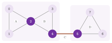
A connected graph may be disconnected by the removal of one node or of one edge, and the parts that survive such removals measure how "reliable" its connections are (e.g., those of a communication network). A cut node (or articulation node) is a node whose removal increases the number of connected components, and a cut edge (or bridge) is an edge with the same property. Two edges are in the same bi-node-connected component, or block, if they are equal or lie on a common cycle; this is an equivalence relation on the edges, whose classes are separated by the cut nodes. Two nodes are in the same bi-edge-connected component if two edge-disjoint paths join them; this is an equivalence relation on the nodes, whose classes are separated by the bridges. For instance, the graph of Figure 18.1 has four blocks (the triangles A and B, which share the cut node 2, the bridge C and the triangle D), three cut nodes and two bi-edge-connected components.
The header provides, for the nodes and for the edges, the same kinds of
function as for the connected components. For the blocks they are
bool biNodeConnected( g ), int countBiNodeConnectedComponents( g ),
int biNodeConnectedComponents( g , compMap ) and
int biNodeConnectedCutNodes( g , cutMap ). For the bi-edge-connected
components they are bool biEdgeConnected( g ),
int countBiEdgeConnectedComponents( g ),
int biEdgeConnectedComponents( g , compMap ) and
int biEdgeConnectedCutEdges( g , cutMap ). Note that the map of the blocks
is an edge map, since a block is a set of edges and a cut node belongs to
several blocks, whereas the map of the bi-edge-connected components is a node
map; both are numbered from \(0\) as in §18.1, consecutively within
a component. Those that find the cut nodes and the cut edges set cutMap to
true on them (once each) and return their number. They leave the other items
untouched, and the caller must therefore initialize the map to false when it
reads the other items too.
abLEMON
biNodeConnectedCutNodes() keeps the nodes it has counted in a map of its
own and only writes cutMap, as the concept check of its argument (a
writable map) requires. In LEMON 1.3.1 it read cutMap in order not to
count a node twice, so that a node already true on entry was neither
counted nor reported; the test connectivity_test passes a map that is
true everywhere. LEMON 1.3.1 also reported every node that carries a
loop as a cut node, e.g., a single node with a loop, and on an
undirected graph parallelFree() returned false on a single loop,
whose two arcs it took for parallel ones; connectivity_test checks
both on graphs with loops.
At the boundary we follow the conventions of the header. A graph with zero or
one node is bi-node-connected, two isolated nodes are not, and two nodes
joined by an edge are. In general, biNodeConnected() returns false if the
graph has an isolated node together with some other node, and otherwise
whether it has at most one block (an isolated node is in no block, since a
block is a set of edges). On the other hand, biEdgeConnected() returns
whether there is at most one bi-edge-connected component; hence, the empty
graph is bi-edge-connected. A loop forms a block of its own (which may be
surprising), but it makes no node a cut node, since the removal of its node
removes it too.
All these functions rely on one depth-first search, with the low points of Hopcroft and Tarjan 1973 and Tarjan 1972. We denote by \(\mathrm{num}(v)\) the index of \(v\) in the order of discovery, by \(T_v\) the subtree of the search rooted at \(v\), and by \(\mathrm{low}(v)\) the least of \(\mathrm{num}(v)\) and of the indices \(\mathrm{num}(x)\) of the nodes \(x\) joined by a non-tree edge to a node of \(T_v\).
Lemma 18.2. In a depth-first search of a connected graph, the root is a cut node if and only if it has at least two children in the tree, and any other node \(u\) is a cut node if and only if it has a child \(w\) with \(\mathrm{low}(w)\ge\mathrm{num}(u)\). The tree edge \(uw\), with \(u\) the parent of \(w\), is a bridge if and only if \(\mathrm{low}'(w)>\mathrm{num}(u)\), where \(\mathrm{low}'\) is computed like \(\mathrm{low}\) but without the edge \(uw\) itself; a non-tree edge is never a bridge.
Proof. By Lemma 18.1, an edge with one end in \(T_w\) and the other outside \(T_w\) is either the tree edge \(uw\) or a non-tree edge to an ancestor of \(w\), i.e., to \(u\) or to an ancestor of \(u\). If \(u\) is not the root and \(\mathrm{low}(w)\ge\mathrm{num}(u)\), no edge leaves \(T_w\) except towards \(u\), and the removal of \(u\) separates \(T_w\) from the parent of \(u\). If, instead, \(\mathrm{low}(w)<\mathrm{num}(u)\) for each child \(w\) of \(u\), each \(T_w\) keeps an edge to a proper ancestor of \(u\) after the removal of \(u\), and the nodes outside \(T_u\) stay connected by the tree edges; hence, \(u\) is not a cut node. For the root, Lemma 18.1 implies that no edge joins the subtrees of two different children, so the removal of the root separates them when there are two or more, and leaves the connected \(T_w\) of a single child \(w\). Finally, the removal of the tree edge \(uw\) disconnects the graph if and only if no other edge leaves \(T_w\), i.e., if and only if \(\mathrm{low}'(w)>\mathrm{num}(u)\). A non-tree edge lies on the cycle that it closes with the tree path between its ends, and its removal disconnects nothing. \(\square\)
In the library, the visitor of the cut nodes applies the lemma as Algorithm 18.1 shows, in which \(\mathrm{pred}(v)\) is the parent of \(v\) in the tree.
Algorithm 18.1 (Cut nodes by the low points).
1  for each node r not yet reached: root := r; rootCut := false; DFS(r)
2  DFS(v): num(v) := low(v) := next index
3     for each arc vw:
4        if w is not reached: pred(w) := v; DFS(w)
5           low(v) := min(low(v), low(w))
6           if num(v) <= low(w):
7              if v != root or rootCut: mark v as a cut node, once
8              else rootCut := true
9        else if w = v: skip the arc                          (a loop)
10       else if w != pred(v): low(v) := min(low(v), num(w))
Steps 2, 4 and 10 are the visitor functions reach(), discover() and
examine() of DfsVisit, and steps 5 to 8 its backtrack(); the flag "once"
is the private map of the note above. Step 7 marks the root at the second of
its children that satisfy the condition of step 6, the flag rootCut
recording the first one. Step 10 skips all the edges to the parent, including
the parallel ones, which does not change the outcome of step 6.
Theorem 18.4. Algorithm 18.1 marks exactly the
cut nodes of the graph, and it costs \(O(n+m)\). The count of the blocks, which
grows by one at each loop and at each tree edge \(vw\) that satisfies the
condition of step 6, is the number of blocks, and
biNodeConnectedComponents() gives the same index to two edges if and only if
they lie in the same block.
Proof. When \(\mathrm{DFS}(w)\) returns, \(\mathrm{low}(w)\) is the least of \(\mathrm{num}(w)\), of the values \(\mathrm{num}(x)\) of step 10 over the arcs leaving \(w\) and of the low points of its children. By induction on the height of \(T_w\), this is the low point of the definition (the arcs of step 10 that lead to descendants have \(\mathrm{num}(x)>\mathrm{num}(w)\) and do not count, and the skipped edges to the parent only add \(\mathrm{num}(\mathrm{pred}(w))\), which leaves the test of step 6 unchanged). The loops, which step 9 skips, lie on no path between two distinct nodes, and hence they neither change the cut nodes nor enter the low points. Since each child of the root satisfies step 6, steps 6 to 8 apply Lemma 18.2 in each component. For the blocks, call a tree edge \(vw\) that satisfies step 6 a closing edge. Removing \(v\) separates \(T_w\) (or, at the root, the subtree of each child), so no cycle contains both an edge of \(T_w\cup\{vw\}\) and an edge outside it. Conversely, the edges of \(T_w\cup\{vw\}\) that are not inside the subtree of a lower closing edge, together with the non-tree edges from those nodes to \(v\) or below, are pairwise on common cycles (each of them closes a cycle through the tree path, and these cycles overlap along tree edges that are not closing). Hence, each closing edge determines one block. The function that numbers them keeps on a stack the edges discovered since the block was opened and pops them when its closing edge is backtracked. The search examines each arc once, and each edge enters and leaves the stack once. \(\square\)
The full proof of the block structure is in Hopcroft and Tarjan 1973 and Tarjan 1972 (see also Cormen et al. 2001, Problem 22-2), whose arguments the proof above follows. In contrast, the functions on the bi-edge-connected components store the arc by which each node was entered and skip only its opposite, since a second edge parallel to a tree edge does give a path back and prevents that edge from being a bridge. They update \(\mathrm{low}(v)\) at a non-tree arc \(vx\) with the current low point of \(x\) rather than with \(\mathrm{num}(x)\), which, as the following proof shows, does not change the test.
Theorem 18.5. In the search of the
bi-edge-connected components, a node \(v\neq\) root satisfies
\(\mathrm{low}(v)=\mathrm{num}(v)\) when it is left if and only if the tree edge
that entered it is a bridge. Hence, biEdgeConnectedCutEdges() marks the
bridges, biEdgeConnectedComponents() numbers exactly the bi-edge-connected
components (the nodes still on a stack when such a \(v\), or a root, is left),
and all four functions cost \(O(n+m)\).
Proof. At a non-tree arc \(vx\), the current low point of \(x\) is at most \(\mathrm{num}(x)\), and it is less than \(\mathrm{num}(v)\) only if \(x\) is outside \(T_v\) or some node of \(T_x\), already examined, has an edge leaving \(T_v\). Hence, \(\mathrm{low}(v)<\mathrm{num}(v)\) holds when \(v\) is left if and only if an edge other than the one that entered \(v\) leaves \(T_v\), which by Lemma 18.2 is the negation of the bridge condition. The removal of all the bridges leaves connected graphs without bridges, whose node sets are the sets popped from the stack. In a connected graph without bridges any two nodes are joined by two edge-disjoint paths, by the edge version of Menger's theorem (Diestel 2017, Theorem 3.3.6), while two nodes separated by a bridge are not. Each arc is examined once and each node is pushed and popped once. \(\square\)
18.3 Strong components and topological order¶
Two nodes of a digraph are strongly connected if directed paths join them in
both directions. This is an equivalence relation, whose classes are the
strongly connected components, and the digraph that has one node per
component, and an arc from one component to another whenever some arc of \(D\)
goes so, is acyclic (we call it the condensation of \(D\)). The library offers
bool stronglyConnected( d ), int countStronglyConnectedComponents( d ),
int stronglyConnectedComponents( d , compMap ) and
int stronglyConnectedCutArcs( d , cutMap ), with the conventions of
§18.1, i.e., the empty digraph is strongly connected and has zero
components. Of these, stronglyConnected() runs a depth-first search from the
first node on \(D\) and another on its reverse (the adaptor ReverseDigraph of
chapter 5), and it checks that both searches reach all
the nodes (which is correct by Theorem 18.1 applied to directed paths: a node
is reached from \(s\) if and only if a directed path joins \(s\) to it). Instead,
the other three functions use the algorithm usually attributed to Kosaraju and
published by Sharir 1981.
Algorithm 18.2 (Strongly connected components by two depth-first searches).
1  run a DFS of D from each node not yet reached, and list the nodes
   in the order in which the search leaves them
2  k := 0
3  for each node v in the reverse of that list:
4     if v is not reached by the second search:
5        run a DFS of the reverse of D from v; give index k to the nodes
         it reaches; k := k + 1
6  return k
For a set \(C\) of nodes we denote by \(f(C)\) the largest position, in the list of step 1, of a node of \(C\).
Lemma 18.3. If an arc of \(D\) goes from a strongly connected component \(C\) to another one \(C'\), then \(f(C)>f(C')\).
Proof. Let \(x\) be the first node of \(C\cup C'\) that the search of step 1 reaches. If \(x\in C\), each node of \(C\cup C'\) is reachable from \(x\) by a directed path of nodes not yet reached, and the search leaves all of them before leaving \(x\); hence, \(f(C)\) is the position of \(x\), larger than any position in \(C'\). If \(x\in C'\), the search of \(x\) reaches all of \(C'\) and no node of \(C\) (a directed path from \(C'\) to \(C\) would merge the two components), and it leaves all of \(C'\) before any node of \(C\) is reached. \(\square\)
Theorem 18.6. Each search of step 5 gives its
index to exactly one strongly connected component, and no arc of \(D\) goes from
a component of higher index to one of lower index. Hence,
countStronglyConnectedComponents() and stronglyConnectedComponents() are
correct, the numbering is a topological order of the condensation, the arcs
that stronglyConnectedCutArcs() marks are the arcs whose ends lie in
different components, and each of the four functions costs \(O(n+m)\).
Proof. Let \(v\) start a search of step 5, and let \(C\) be its component. All of \(C\) is reachable from \(v\) in the reverse digraph, and none of it was reached by an earlier search, since an earlier search would have started from a node of larger position and, by induction, collected its own component only. An arc of the reverse digraph that leaves \(C\) corresponds to an arc of \(D\) that enters \(C\) from a component \(C''\), and by Lemma 18.3 \(f(C'')>f(C)\); hence \(C''\) contains a node of larger position than \(v\), and by induction it was collected by an earlier search. Thus the search from \(v\) reaches \(C\) and nothing else. The components are numbered in decreasing order of \(f\), so an arc from \(C\) to \(C'\), for which \(f(C)>f(C')\), goes from a lower index to a higher one. The cut arcs are found in the second pass: when an arc of the reverse digraph is examined, its other end is either in the current component or in one already numbered, and the arc is marked if the two indices differ. Each pass examines each arc once. \(\square\)
The function stronglyConnectedCutArcs() sets its arcs to true in cutMap,
leaves the other arcs untouched (the map must start at false), and returns
their number. The proof is the one of Cormen et al. 2001,
§22.5 (Lemma 22.14 and Theorem
22.16), with the list of step 1 in place of the finishing times.
A digraph without directed cycles is a DAG, and a topological order of a
DAG is a numbering of its nodes in which each arc goes from a lower to a
higher number. Three functions deal with them, i.e., bool dag( d ),
void topologicalSort( d , order ) and
bool checkedTopologicalSort( d , order ). The first one runs a depth-first
search from each unreached node and returns false at the first arc whose
target has been reached but not yet left (a back arc; a loop is one). Next,
topologicalSort() writes in the writable node map order the values from
\(n-1\) down to \(0\), in the order in which a depth-first search leaves the
nodes, each value once. It does not check that the digraph is a DAG, which is
its precondition. By contrast, checkedTopologicalSort() does check it, and
it needs a map that can also be read: it first sets all the values to \(-1\),
and it returns false at the first arc that leads to a node reached and still
at \(-1\) (i.e., not yet left), leaving the map partly written.
Theorem 18.7. A digraph has a directed cycle
if and only if a depth-first search of it meets a back arc. Hence, dag() and
checkedTopologicalSort() return false if and only if the digraph has a
directed cycle; on a DAG, topologicalSort() and checkedTopologicalSort()
give order[u] < order[v] for each arc \(uv\). All three cost \(O(n+m)\).
Proof. A back arc \(uv\) goes to a node \(v\) that is still active, i.e., to an ancestor of \(u\) in the tree, and it closes a directed cycle with the tree path from \(v\) to \(u\). Conversely, let \(C\) be a directed cycle and \(v\) its first node reached; all the other nodes of \(C\) are reachable from \(v\) through unreached nodes, and they become descendants of \(v\), so that the arc of \(C\) that enters \(v\) is examined while \(v\) is active, and it is a back arc. On a DAG there is no back arc, so when an arc \(uv\) is examined, \(v\) is either unreached (and then it becomes a descendant of \(u\) and is left before \(u\)) or already left. In both cases \(v\) is left before \(u\), and since the values are given in decreasing order of leaving, \(\mathrm{order}(u)<\mathrm{order}(v)\). \(\square\)
One usually runs these functions, or the strongly connected components, before
an algorithm that assumes a DAG or a strongly connected digraph; for instance,
the minimum mean cycle algorithms of chapter 16
call stronglyConnectedComponents() and then work on one component at a time.
The program manual/examples/18-components.cc (the test
manual_18_components) builds the graph of Figure 18.1 and
checks the numbers of its components, blocks, cut nodes and bridges. It then
checks that the numbering of the strongly connected components of a digraph
with three of them is a topological order of the condensation, and sorts a
"small" DAG.
18.4 Euler tours¶
An Euler tour of a graph is a closed walk that traverses each edge once (for a digraph, each arc in its direction). We recall its characterization, which is the oldest theorem of graph theory, and we prove it after the algorithm, whose analysis gives the sufficiency.
Theorem 18.8. A graph whose edges lie in one connected component has an Euler tour if and only if each node has even degree. A digraph whose arcs lie in one connected component of the underlying undirected graph has an Euler tour if and only if each node has as many entering arcs as leaving ones.
The proof of sufficiency, due to Hierholzer and Wiener
1873, is also the algorithm:
from any node, a walk that never reuses an arc can stop only at its starting
node, and a closed walk that misses some arc can be extended by splicing into
it a closed walk from one of its nodes. In abLEMON the tour is given by an
iterator, DiEulerIt< GR > for a digraph and EulerIt< GR > for an
undirected graph. It is constructed from the graph and, optionally, from the
starting node (by default INVALID, which stands for the first node that has
a leaving arc), and it is advanced with ++ until it compares equal to
INVALID (operator== and operator!= with INVALID test whether the tour
is over). DiEulerIt converts to GR::Arc, while EulerIt converts to
GR::Arc and to GR::Edge, and it gives arcs in order to show in which
direction each edge is traversed; after the end, both convert to INVALID. As
for the other iterators of the library, the postfix ++ returns the current
arc instead of the iterator. A digraph can also be given to EulerIt through
the adaptor Undirector, and an undirected graph to DiEulerIt, which then
treats its arcs as those of a symmetric digraph.
Algorithm 18.3 (Euler tour, as DiEulerIt
produces it).
1  for each node v: next(v) := first arc leaving v
2  L := empty list; s := start
3  while next(s) != INVALID: append next(s) to L; advance next(s);
                             s := target of the arc appended
4  (operator Arc) the current arc is the first of L
5  (operator++) s := target of the first arc of L; remove it from L;
6     while next(s) != INVALID: insert next(s) at the front of the rest
      of L, after the arcs inserted before; advance next(s);
      s := target of that arc
The constructor walks greedily from the start (step 3), and each increment
splices, right after the arc just given, the closed walk that starts where
that arc ends and uses the arcs not yet taken (step 6). EulerIt works in the
same way with an edge map that marks the edges already used, since each edge
appears as an arc leaving each of its two ends, and it skips the arcs of the
marked edges when it advances \(\mathrm{next}(v)\). We call a digraph balanced
if each node has as many entering arcs as leaving ones, and an undirected
graph balanced if each degree is even.
Lemma 18.4. In a balanced graph, a walk from \(s\) that uses each arc (edge) at most once and stops when its current node has no unused arc stops at \(s\), and the unused arcs form a balanced graph again.
Proof. Each time the walk enters a node \(x\neq s\), it has used one more arc entering \(x\) than arcs leaving it (for an undirected graph, an odd number of the edges of \(x\)), so by the balance an unused arc leaves \(x\) and the walk does not stop there. The used arcs form a closed walk, which enters and leaves each node equally often; their removal keeps the balance. \(\square\)
Theorem 18.9. If the graph is balanced, its arcs (edges) lie in one connected component of the underlying undirected graph, and the start has a leaving arc, the iterators give an Euler tour that starts at the start. In all cases they cost \(O(n+m)\) for the whole walk.
Proof. Let \(W\) be the sequence of the arcs already given followed by \(L\). By
Lemma 18.4, after the constructor \(W\) is a closed walk from the start that
repeats no arc. At an increment the first arc of \(L\), say \(uv\), is given, and
step 6 is the walk of Lemma 18.4 from \(v\) on the unused arcs, which are
balanced; it is closed at \(v\), and its insertion right after \(uv\) keeps \(W\) a
closed walk that repeats no arc. Furthermore, step 3 or step 6 stops at a node
whose pointer is INVALID, which is the node where the walk started; hence,
when the iteration ends, each node that \(W\) visits has no unused leaving arc.
Suppose that an arc is unused at the end; since the arcs lie in one connected
component, some node \(t\) visited by \(W\) is joined by an unused arc to a node
not visited. The arc cannot leave \(t\), so it enters \(t\); but \(W\) is closed and
contains all the arcs leaving \(t\), hence as many arcs entering \(t\) as the
balance allows, i.e., all of them, a contradiction. The pointers
\(\mathrm{next}(v)\) only advance and each arc enters \(L\) once, while the
initialization of the pointers (and of the edge map of EulerIt) costs
\(O(n)\). \(\square\)
Proof of Theorem 18.8. A closed walk enters each node as often as it leaves it (and, undirected, uses an even number of its edge ends), so the condition is necessary. Theorem 18.9 shows that it suffices. \(\square\)
If the graph has no Euler tour, the iterators still give a walk (possibly a
rather short one), which is not closed or does not contain all the edges, and
from which one can usually tell little. One should therefore check the
property first, with bool eulerian( g ), which works on digraphs and on
undirected graphs (the two versions are selected through the undirected tag of
the graph type). On an undirected graph it returns true if each node has
even degree (countIncEdges(), which counts a loop twice) and the graph is
connected; on a digraph, if each node has as many entering as leaving arcs and
the underlying undirected graph (the adaptor Undirector) is connected. Both
checks cost \(O(n+m)\). We remark that eulerian() requires that all the nodes
be connected, whereas Theorem 18.8 requires it of the edges only; thus, a
graph with an Euler tour and an isolated node is not Eulerian for the
function, as its documentation warns. The program
manual/examples/18-euler.cc (the test manual_18_euler) follows the tour of
the complete graph on five nodes by EulerIt and that of two directed
triangles sharing a node by DiEulerIt. It checks each to be a closed walk
through every edge or arc once, and checks that an isolated node makes
eulerian() false while the tour is still there.
18.5 Planarity, embedding and drawing¶
We recall that a graph is planar if it can be drawn in the plane with no two edges crossing. Up to deformation, such a drawing is described by its combinatorial embedding, i.e., by the cyclic order of the edges around each node (e.g., counterclockwise in the drawing). In turn, the faces of the drawing are the orbits of the map that takes an arc \(uv\) to the arc that follows \(vu\) around \(v\), i.e., the walks along the boundaries of the regions into which the drawing cuts the plane. We first state the counting facts that the algorithms of this section and of §18.6 use.
Lemma 18.5. A connected plane graph with \(n\) nodes, \(m\) edges and \(f\) faces satisfies \(n-m+f=2\) (Euler's formula). Hence, a planar simple graph with \(n\ge3\) nodes has \(m\le3n-6\) edges, and every planar simple graph has a node of degree at most five.
Proof. We argue by induction on \(m\). A tree has \(m=n-1\) and one face. If the graph is not a tree, an edge \(e\) of a cycle has, by the Jordan curve theorem, different faces on its two sides, and its removal leaves a connected plane graph with one edge and one face less (see Diestel 2017, Theorem 4.2.9). For the bound we may add edges until the graph is connected, which keeps it planar and simple. In a simple graph with \(n\ge3\) nodes each face is bounded by a walk of at least three edges, and each edge lies twice on these walks; hence \(2m\ge3f\), and Euler's formula gives \(m\le3n-6\). Finally, the degrees sum to \(2m\le6n-12<6n\), so some node has degree at most five (with fewer than three nodes, each degree is at most one). \(\square\)
Furthermore, the obstacles to planarity are known.
Theorem 18.10. A graph is planar if and only if it contains no subdivision of \(K_5\) (the complete graph on five nodes) and no subdivision of \(K_{3,3}\) (the complete bipartite graph with three nodes on each side).
Proof sketch. Neither graph is planar: \(K_5\) has \(10>3\cdot5-6\) edges (Lemma 18.5), and \(K_{3,3}\), being bipartite, has faces of at least four edges, hence \(2m\ge4f\) and \(m\le2n-4=8<9\). A subdivision of a nonplanar graph is nonplanar, and so is a graph that contains it. The converse, i.e., that a nonplanar graph contains one of the two subdivisions, is the theorem of Kuratowski 1930. Its proof, by a minimal counterexample that is shown to be 3-connected and then embedded around a contracted edge, is given in Diestel 2017, §4.4, Theorem 4.4.6. \(\square\)
A subdivision of either graph inside a nonplanar graph, called a Kuratowski
subdivision, certifies that the graph is not planar, as an embedding
certifies that it is. We now describe the implementation of the algorithm of
Boyer and Myrvold 2004, which
computes either an embedding or a Kuratowski subdivision, and which is usually
regarded as one of the simplest linear planarity tests. The function
bool checkPlanarity( g ) runs a simplified version of it that builds neither
certificate, and the class PlanarEmbedding< Graph > runs the full one. Both
expect an undirected simple graph (a precondition of the constructor), which
simpleGraph() of §18.1 checks. Once the class is constructed
from the graph, run( bool kuratowski = true ) returns whether the graph is
planar. If it is, next( a ) gives the arc that follows the arc a in the
cyclic order of the arcs leaving its source, and embeddingMap() returns the
whole order as a const reference to an arc map of arcs (the type
EmbeddingMap, i.e., Graph::ArcMap< Arc >). If it is not, and run() was
called with true, kuratowski( e ) returns whether the edge e belongs to
the subdivision found, whose nodes of degree three or four are those of a
\(K_{3,3}\) or of a \(K_5\) (with false, or before run(), it returns false
on every edge).
Algorithm 18.4 (Planarity by edge addition,
outline of PlanarEmbedding::run()).
1  run a DFS; record the order of discovery, the tree edges, the low points
   and, for each node, the least ancestor joined to it by a back edge;
   sort the children of each node by their low points (radixSort)
2  for each node v in reverse order of discovery:
3     embed each tree edge from v to a child as a separate biconnected
      component, rooted at a virtual copy of v
4     for each back edge from a descendant w to v: walk up from w and mark
      the components that the edge will cross (walkUp)
5     for each marked root: walk down along the external faces, embedding
      the back edges to v and merging the components on the way, flipping
      a component when its orientation requires it (walkDown)
6     if a back edge to v is left unembedded:
         if kuratowski: isolate a Kuratowski subdivision
         return false
7  merge the remaining components and store the cyclic orders; return true
Theorem 18.11. PlanarEmbedding::run() and
checkPlanarity() return true if and only if the simple graph is planar; in
that case embeddingMap() is a combinatorial embedding of a plane drawing,
and otherwise, after run( true ), the edges marked by kuratowski() form a
Kuratowski subdivision. The sort of step 1 costs \(O(n\log n)\) in all, and the
rest of the method \(O(n+m)\), which is \(O(n)\) on a planar simple graph.
Proof sketch. The invariant, proved by Boyer and Myrvold
2004, is that after processing \(v\)
the tree, together with the back edges to the nodes processed so far, is
embedded with each node that still has a back edge to an unprocessed ancestor
on the external face of its component. The walk-down of step 5 embeds each
back edge to \(v\) that some embedding with this property can accommodate, and
it fails only when none can; at that point the obstruction it meets is
completed, along the external faces and the tree paths, to a subdivision of
\(K_{3,3}\) or of \(K_5\). For the cost, the children of a node are sorted by
radixSort() of chapter 8, which costs \(O(k\log n)\)
for \(k\) children with low points below \(n\), and the \(n-1\) children of all the
nodes give \(O(n\log n)\) (the paper sorts by buckets in linear time). The flips
of step 5 are recorded lazily, with one flag per component, and each step of
the walks is charged to an edge embedded or to a face boundary shortened,
which keeps the rest linear. On a nonplanar graph the method stops at the
first node at which a back edge is left unembedded. \(\square\)
The documentation of PlanarEmbedding states the same bound.
The class PlanarDrawing< Graph > computes a straight-line drawing on an
integer grid by the method of Schnyder
1990. Its coordinates have the
type dim2::Point< int > (the type Point, stored in the node map type
PointMap), and its interface is the constructor from a simple graph and the
two functions run() and run( embedding ). Of these, the former computes an
embedding with PlanarEmbedding and returns false if the graph is not
planar; the latter, a template on the type of the map, draws according to a
given combinatorial embedding (e.g., embeddingMap() of a PlanarEmbedding)
and has no return value. Then the coordinates are read with
operator[]( node ) or, as a node map, with coords(). On a graph with
\(m=3n-6\), run( embedding ) draws the graph itself; on any other graph it
copies the graph into an edge set and adds edges, consistently with the
embedding, to make it connected, then bi-node-connected and then maximal
planar, draws the triangulation and keeps the coordinates of the nodes. A
graph with fewer than three nodes is drawn on a vertical line, with \(x=0\) and
\(y=0,1\).
Theorem 18.12. For a planar simple graph with
\(n\ge3\) nodes and a combinatorial embedding of a plane drawing,
PlanarDrawing::run( embedding ) places the nodes at distinct points of the
grid \([0,n-2]\times[0,n-2]\) so that the straight segments of the edges do not
cross.
Proof sketch. A maximal planar graph (a triangulation, with \(m=3n-6\)) has a realizer, i.e., a partition of its inner edges into three trees, rooted at the three nodes of the outer face, such that around each inner node the edges of the three trees appear in a fixed cyclic pattern. The three paths from a node to the three roots split the triangle into three regions, and the numbers of nodes in two of them (less the nodes on their boundary paths) are integer coordinates in \([0,n-2]\), for which each face is a non-degenerate triangle with the orientation of the embedding. This is the main theorem of Schnyder 1990; the edges added to reach a triangulation are dropped afterwards, which removes segments and creates no crossing. The header states a time of \(O(n)\). \(\square\)
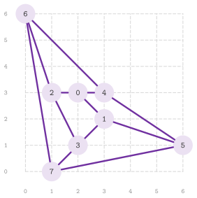
The grid is somewhat small (of side \(n-2\)), which is often convenient for a picture, although some angles between edges may be quite sharp. Figure 18.2 shows the drawing of the cube that the program of the next section computes.
abLEMON
In LEMON 1.3.1, PlanarDrawing::run() without arguments passed the
PlanarEmbedding object, instead of its embedding map, to
run( embedding ), and therefore did not compile once instantiated.
abLEMON has the correction made in the repository of LEMON after that
release (trac #610), as well as the drawing of the graphs with fewer than
three nodes (trac #611), on which the algorithm failed.
18.6 Coloring planar graphs¶
We call coloring of a graph an assignment of a color to each node, with
different colors at the ends of each edge. As is well known, every planar
graph can be colored with four colors, by the theorem of Appel and Haken
1977, whose proof yields a quadratic
algorithm that the header judges of no practical use. Deciding whether a
planar graph can be colored with three colors is NP-complete (Garey, Johnson
and Stockmeyer 1976), and two colors,
when they suffice, are found by bipartitePartitions() of §18.1.
The class PlanarColoring< Graph > computes colorings with six and with five
colors, both from the order in which the nodes are removed from the graph when
one always takes a node of least degree among the remaining ones (a
smallest-last order, cf. Matula and Beck
1983).
Lemma 18.6. In the smallest-last order of a planar simple graph, each node has at most five neighbors that are removed after it.
Proof. When a node is removed it has the least degree in the remaining graph, which is planar and simple, and therefore it has at most five neighbors left, by Lemma 18.5. \(\square\)
Hence, one can give the colors greedily in the reverse of that order, which is
what Algorithm 18.5 does; there \(k=6\) for runSixColoring() and \(k=5\) for
runFiveColoring().
Algorithm 18.5 (Coloring of a planar graph with six or five colors).
1  repeatedly remove a node of least degree in the remaining graph
   (a bucket heap keyed by the degree), and record the order
2  for each node v in the reverse of that order:
3     give v the least color in {0,..,k-1} not used by its colored
      neighbors
4     if there is none (k = 6): return false
5     if there is none (k = 5): take the first four colored neighbors
      u1, u2, u3, u4 of v in the cyclic order of the embedding;
6        if the Kempe chain of u1 (the component of the colors of u1, u3
         that contains u1) does not contain u3: swap its two colors,
         and give v the old color of u1
7        else swap the colors in the Kempe chain of u2 (colors of u2 and
         u4), and give v the old color of u2
Theorem 18.13. runSixColoring() costs
\(O(n+m)\); on a planar simple graph it returns true with a coloring by at
most six colors, and when it returns false the graph is not planar (although
true does not prove that it is).
Proof. By Lemma 18.6, when \(v\) is colored at most five of its neighbors are colored, so step 3 succeeds with six colors on a planar simple graph, and the contrapositive gives the second claim. A node is colored differently from the neighbors colored before it, and the neighbors colored after it avoid its color, so the coloring is proper. The heap receives \(n\) insertions, \(n\) deletions of the minimum and at most \(2m\) decreases, each of which lowers a key by one. Hence the minimum of the bucket heap moves back by at most one per decrease, and its forward moves are bounded by these plus the largest degree, which gives \(O(n+m)\) with the \(O(n+m)\) of step 2. \(\square\)
Theorem 18.14. Given a planar simple graph
and a combinatorial embedding of a plane drawing of it,
runFiveColoring( embedding ) computes a coloring with at most five colors in
\(O(n(n+m))=O(n^2)\) time.
Proof. Step 3 fails only when the colored neighbors of \(v\), at most five by
Lemma 18.6, use all five colors; then they are five, \(u_1,\ldots,u_5\) in the
cyclic order around \(v\), with distinct colors \(c_1,\ldots,c_5\). Note that a
swap of the two colors of a Kempe chain, i.e., of a connected component of the
subgraph induced by the colored nodes of those two colors, keeps the coloring
proper. If the chain of \(u_1\) does not contain \(u_3\), the swap gives \(u_1\) the
color \(c_3\) and leaves \(u_3\) (and the neighbors \(u_2,u_4,u_5\), of other
colors) unchanged, so that \(c_1\) becomes free at \(v\). Otherwise a path of
colors \(c_1,c_3\) joins \(u_1\) to \(u_3\), and with \(v\) it forms a cycle of the
plane drawing. Since \(u_2\) and \(u_4\) lie between \(u_1\) and \(u_3\) on the two
sides of the cyclic order, the Jordan curve theorem puts them on different
sides of the cycle, and a path of colors \(c_2,c_4\) from \(u_2\), which meets no
node of the cycle, cannot reach \(u_4\). Hence the swap of the chain of \(u_2\)
frees \(c_2\) at \(v\). This is the argument of Kempe
1879, as Heawood
1890 restricted it to five colors (see
also Diestel 2017, Proposition
5.1.2). In fact, each recoloring is a
breadth-first search of an adaptor FilterNodes of the graph, which costs
\(O(n+m)\), and it happens at most once per node; the rest is as in Theorem
18.13. \(\square\)
As for its interface, PlanarColoring has the constructor from a simple graph
and three functions to compute a coloring. Of these, runSixColoring() is the
one of Theorem 18.13; runFiveColoring( embedding ), a template on the type
of the map, needs a combinatorial embedding and has no return value; and
runFiveColoring() computes the embedding with PlanarEmbedding, returns
false on a nonplanar graph, and costs in addition the time of Theorem 18.11.
One reads the results with colorIndex( node ), between \(0\) and \(4\) or \(5\),
and with color( node ), a Color of a palette of six (red, green, blue,
yellow, magenta and cyan, in the order of the indices). As maps,
colorIndexMap() returns a const reference to the node map of the indices
(the type IndexMap), and colorMap() the map of the colors (the type
ColorMap, a ComposeMap of the palette and of the indices). Both
PlanarDrawing and PlanarColoring also export the item and iterator types
of the graph (Node, Arc, NodeIt, and so on).
abLEMON
PlanarColoring::colorIndexMap() returns a const reference to the map of
the color indices; in LEMON 1.3.1 it returned a copy of it, made in \(O(n)\)
at each call.
The program manual/examples/18-planar.cc (the test manual_18_planar)
computes the embedding of the cube and counts its faces against Euler's
formula. It then draws the cube on the grid, checks that no two edges cross,
colors it with six and with five colors, and finds the Kuratowski subdivision
of \(K_{3,3}\), which coincides with \(K_{3,3}\).
18.7 Subgraph isomorphism: VF2 and VF2++¶
Given two undirected graphs \(G_1=(V_1,E_1)\) and \(G_2=(V_2,E_2)\), with
\(n_1=|V_1|\) and \(n_2=|V_2|\), a mapping (or embedding) is an injective
function \(f:V_1\to V_2\). In the Subgraph Isomorphism Problem one looks for a
mapping with \(f(u)f(v)\in E_2\) whenever \(uv\in E_1\), and in the Induced
Subgraph Isomorphism Problem one requires, furthermore, that \(f(u)f(v)\notin
E_2\) whenever \(uv\notin E_1\). In the Graph Isomorphism Problem the induced
mapping must also be bijective. When the nodes carry labels \(l_1:V_1\to L\) and
\(l_2:V_2\to L\), one also requires that \(l_1(u)=l_2(f(u))\) for each \(u\in V_1\).
An enumeration MappingType (in the namespace lemon, from
lemon/bits/vf2_internals.h) selects the problem, with the values SUBGRAPH
(the default), INDUCED and ISOMORPH. According to the header, ISOMORPH
is equivalent to INDUCED when the two graphs have the same number of nodes,
and to SUBGRAPH when they also have the same number of edges, but it may be
faster than both, since its cutting rules are stronger. For ISOMORPH,
find() compares \(n_1\) with \(n_2\) first and returns false when they differ,
since otherwise the search would give the induced mappings that preserve the
degrees, i.e., the isomorphisms of \(G_1\) onto a union of connected components
of \(G_2\) (e.g., four mappings of one edge into two disjoint edges). Both
classes require simple graphs, as their headers state: a pair of parallel
edges in \(G_2\) makes a candidate appear twice, and the same mapping is then
reported twice.
Of course, the subgraph isomorphism problem is NP-complete, since it contains the clique problem. Hence, the two algorithms of this section are backtracking searches that may take exponential time, and their speed in practice depends mostly (and often decisively) on the order in which they consider the nodes of \(G_1\) and on the rules with which they cut the search tree. We now give the search common to both, in which \(\mathrm{conn}(w)\), for a node \(w\) of \(G_2\), is \(-1\) if \(w\) is the image of a node already mapped and otherwise the number of its neighbors that are such images.
Algorithm 18.6 (VF2 and VF2++ search,
find()).
1  order the nodes of G1 as v_0, .., v_{n1-1} (VF2: breadth first from
   each unreached node; VF2++: see the text)
2  depth := 0; all the nodes of G1 unmapped
3  while depth >= 0:
4     if depth = n1: depth -= 1; return true (the mapping is in m)
5     u := v_depth; take the next candidate w for u, after the one tried
      last (whose pair is undone first): if u has a mapped neighbor, the
      neighbors w of the image of the first of them with conn(w) > 0;
      else the nodes w of G2 with conn(w) >= 0 (SUBGRAPH) or
      conn(w) = 0 (INDUCED, ISOMORPH), in the order of NodeIt
6     if there is none: unmap u; depth -= 1; continue
7     if feasible(u, w): map u to w, update conn; depth += 1
8  return false
The test feasible( u , w ) checks the label (or the equivalence of the
nodes), and it checks that each mapped neighbor of \(u\) has its image among the
neighbors of \(w\) and, for INDUCED and ISOMORPH, that each mapped neighbor
of \(w\) is such an image. It then looks ahead. With the numbers
\(r^{\mathrm{io}}(u)\) of the unmapped neighbors of \(u\) adjacent to the mapped
part and \(r^{\mathrm{new}}(u)\) of the others (precomputed for \(u\) along the
order), and with the same numbers for \(w\), read from \(\mathrm{conn}\), it
requires \(r^{\mathrm{io}}(u)\le r^{\mathrm{io}}(w)\), also
\(r^{\mathrm{new}}(u)\le r^{\mathrm{new}}(w)\) for INDUCED, and both
equalities for ISOMORPH. We call admissible the mappings of the type (with
the labels), where for ISOMORPH this means an isomorphism, i.e., an induced
mapping with \(n_1=n_2\), which then preserves the degrees.
Theorem 18.15. On simple graphs, the
successive calls of find() return each admissible mapping exactly once, and
then false.
Proof. The search is a depth-first enumeration of the partial mappings of
\(v_0,\ldots,v_{k-1}\). Step 7 maps \(v_k\) only to a \(w\) for which the partial
mapping stays consistent on the mapped nodes (labels, edges, and for the
induced types non-edges); at depth \(n_1\) the mapping is therefore admissible
for SUBGRAPH and INDUCED, and for ISOMORPH the equalities of the
look-ahead give \(\deg(w)=\deg(u)\) at each step. Conversely, let \(f\) be
admissible and assume that its restriction to \(v_0,\ldots,v_{k-1}\) has been
built. If \(v_k\) has a mapped neighbor \(x\), then \(f(v_k)\) is an unmapped
neighbor of \(f(x)\) with \(\mathrm{conn}>0\); otherwise \(f(v_k)\) is unmapped and,
for the induced types, adjacent to no image. In both cases it is a candidate
of step 5. It passes the consistency test, and it passes the look-ahead, since
\(f\) maps the unmapped neighbors of \(v_k\) injectively into those of \(f(v_k)\),
keeping (for the induced types) their adjacency to the mapped part, and onto
them for ISOMORPH, where the degrees are equal. Hence the search reaches
\(f\). Each candidate is tried once at its depth, since the candidates are
scanned by an iterator whose position is kept between calls (the incident edge
of step 5, stored per depth, or the node that follows the current image in the
order of NodeIt), and since in a simple graph the neighbors of a node are
distinct. A call returns at depth \(n_1\) and the next one resumes from the last
candidate of \(v_{n_1-1}\). \(\square\)
Theorem 18.16. Let \(\Delta_1\) and \(\Delta_2\)
be the largest degrees of \(G_1\) and of \(G_2\). A complete enumeration by
find() examines at most \(P=\sum_{k=0}^{n_1}n_2(n_2-1)\cdots(n_2-k+1)\)
partial mappings and costs \(O(P\,n_2(\Delta_1+\Delta_2))\), i.e., exponential
in \(n_1\) in the worst case; the constructor of Vf2 costs \(O(n_1+m_1+n_2)\),
that of Vf2pp \(O(n_1^2+m_1+n_2+K)\), with \(K\) the largest label plus one.
Proof. The partial mappings of depth \(k\) are injections of \(k\) nodes, at
most \(n_2(n_2-1)\cdots(n_2-k+1)\) of them. At each of them step 5 scans at most
\(n_2\) candidates (the nodes of \(G_2\), or the neighbors of one node). The test
of step 7 and the update of \(\mathrm{conn}\) visit the edges of \(u\) and of \(w\)
a constant number of times (VF2++ also visits the lists of labels of \(u\),
which are not longer than its degree). The order of Vf2 is one breadth-first
search, the precomputed numbers take one pass over the edges, and the map
\(\mathrm{conn}\) is initialized in \(O(n_2)\). The order of Vf2pp chooses the
root of each tree by a scan of the nodes and sorts each level of the tree by
selection, which costs \(O(n_1^2)\) in all, while its counts of the labels are
vectors indexed by the label. \(\square\)
The class Vf2< G1 , G2 , M , NEQ > implements the algorithm of Cordella et
al. 2004. Its first two template
parameters are the type of the graph to be embedded (G1, by default
ListGraph) and that of the graph it is embedded into (G2, by default
ListGraph). The other two are the type of the read-write node map of \(G_1\)
that stores the mapping (M, by default G1::NodeMap< G2::Node >) and a
binary functor on a node of \(G_1\) and one of \(G_2\) that decides whether the
first may be mapped to the second (NEQ, by default a functor that always
returns true). Its constructor Vf2( g1 , g2 , m , neq = NEQ() ) computes
the order of step 1 and the numbers of the look-ahead, and sets all the values
of m to INVALID. Then mappingType() returns the type and
mappingType( t ) sets it, and find() searches for the next mapping, writes
it into m and returns true, or returns false when none is left (and then
m is INVALID again everywhere). The destructor deletes the map only when a
wizard allocated it (see below).
The class Vf2pp< G1 , G2 , M , M1 , M2 > implements the algorithm of
Jüttner and Madarasi 2018, which differs from
VF2 in two respects. First, its labels are integer node maps (M1 and M2,
by default G1::NodeMap< int > and G2::NodeMap< int >), and there is no
functor of node equivalence. The header asks the labels to be \(0,1,\ldots,K-1\)
for \(K\) distinct labels, since the algorithm keeps vectors indexed by the
label, of length the largest label plus one (any nonnegative values work, at
the price of longer vectors). Second, the order of step 1 is chosen to "fail
early". Each breadth-first tree starts from an unordered node whose label is
the "rarest" among the nodes of \(G_2\) (among those, one of largest degree).
Within each level of the tree the nodes are taken by most neighbors already
ordered, then by largest degree, then by rarest label; the look-ahead of
feasible() compares the numbers \(r^{\mathrm{io}}\) and \(r^{\mathrm{new}}\)
label by label. According to the experiments of Jüttner and Madarasi
2018, these two changes typically reduce the
search considerably, especially on labeled graphs; we have not measured the
two classes against each other, and on "easy" instances the difference may
well be small. Its constructor is Vf2pp( g1 , g2 , m , labels1 , labels2 ),
and mappingType(), find() and the destructor are as for Vf2.
Both algorithms also have a function-type interface, vf2( g1 , g2 ) and
vf2pp( g1 , g2 ), which return objects of the classes Vf2Wizard and
Vf2ppWizard (built on the base classes Vf2WizardBase and
Vf2ppWizardBase, which hold the graphs and the parameters). Their named
parameters are mapping( m ), the map that receives the result (by default, a
map is allocated and deleted inside), and nodeLabels( l1 , l2 ). The latter
takes two node maps whose values vf2() compares with == and which
vf2pp() takes as integer labels as above (without them, vf2() may map any
node to any node, and vf2pp() gives all the nodes the label \(0\)). The others
are nodeEq( f ), the functor (for vf2() only), and mappingType( t ),
induced() and iso(). Such an expression ends with run(), which returns
whether a mapping exists and leaves it in the map given by mapping(), with
count(), which returns the number of mappings, or with getPtrToVf2Object()
(respectively getPtrToVf2ppObject()). This last function returns a pointer
to a new algorithm object, on which one calls find() repeatedly and which
the caller deletes; the object then deletes the maps that the wizard
allocated, if any. We remark that both classes work on undirected graphs only
(they iterate on the incident edges), and that the count of the mappings onto
a graph with symmetries includes its automorphisms (e.g., the cycle on five
nodes has 10 automorphisms). Of course, on the same input the two algorithms
give the same set of mappings, possibly in another order; Vf2 remains the
one to use when a functor of node equivalence is more "natural" than integer
labels.
abLEMON
Vf2 and Vf2pp were added to the repository of LEMON after the release
of 1.3.1 (trac #597) and were never in a release of LEMON, so that abLEMON
is the first release that contains them. Furthermore, abLEMON reads the
connection counter of the image of a neighbor only when the neighbor is
mapped, where the code indexed a node map with INVALID (trac #672).
Also, getPtrToVf2Object() and getPtrToVf2ppObject() compile, the
wizards being friends of the classes whose flags of deallocation they set
(trac #682); and lemon/vf2pp.h includes lemon/list_graph.h, whose
ListGraph its default arguments name, so that each of the two headers is
self-contained. In the code of the repository, ISOMORPH did not compare
\(n_1\) with \(n_2\), so that, e.g., vf2( g1 , g2 ).iso().count() was 4 for
one edge and two disjoint edges; vf2_test checks that it is 0, with both
classes.
The program manual/examples/18-isomorphism.cc (the test
manual_18_isomorphism) counts the automorphisms of the cycle on five nodes
and the embeddings of a path of three nodes into the cycle on four nodes and
into \(K_4\), as subgraphs and as induced subgraphs (into \(K_4\) there are 24 of
the former and none of the latter, since any two nodes of \(K_4\) are adjacent).
It then repeats the counts with labels, and enumerates the mappings one by one
with find(), by the class and through the wizard, checking each of them.
18.8 Exercises¶
Exercise 18.1. Add the edge 1-6 to the graph of
Figure 18.1, and predict by Lemma 18.2 the blocks, the cut nodes
and the bridges of the new graph. Check the prediction with the functions of
§18.2, starting from the program
manual/examples/18-components.cc (the test test/connectivity_test.cc
checks the same functions on other graphs).
Exercise 18.2. Build the condensation of a
digraph from the map of stronglyConnectedComponents(), with one node per
component and one arc per cut arc of stronglyConnectedCutArcs(). Verify with
dag() and checkedTopologicalSort() that it is acyclic and that the indices
of the components are a topological order of it, as Theorem 18.6 states (the
program manual/examples/18-components.cc checks the second property on the
original digraph).
Exercise 18.3. A connected graph with two nodes
of odd degree, \(s\) and \(t\), has an Euler path from \(s\) to \(t\). Obtain it with
EulerIt by adding a new edge \(ts\), starting the tour at \(s\) and dropping the
new edge from the walk, and check the result as the program
manual/examples/18-euler.cc checks a tour (the test test/euler_test.cc
checks the iterators on several graphs).
Exercise 18.4. Show that the faces of an
embedding of a planar graph with \(c\) connected components, counted as in the
program manual/examples/18-planar.cc (one orbit per face of each component),
satisfy \(f+n-c=m+1\), and verify it on a graph with two components; the test
test/planarity_test.cc checks this identity in checkEmbedding().
Exercise 18.5. Run PlanarEmbedding on \(K_5\)
and on the Petersen graph, and check that the edges marked by kuratowski()
form a subdivision of \(K_5\) (five nodes of degree four) or of \(K_{3,3}\) (six
nodes of degree three), the other nodes having degree zero or two in it; the
test test/planarity_test.cc makes this check in checkKuratowski().
Exercise 18.6. Count with
vf2( g , g ).iso().count() and with vf2pp( g , g ).iso().count() the
automorphisms of the cube and of the Petersen graph (48 and 120), and compare
the number of calls of find() with and without labels that distinguish one
node. The program manual/examples/18-isomorphism.cc does the same on the
cycle on five nodes, and the test test/vf2_test.cc checks the mappings found
by both classes.
Exercise 18.7. Show that, for a pattern \(G_1\)
that is a complete graph, the counts of the SUBGRAPH and of the INDUCED
mappings into any \(G_2\) coincide, and that, for a pattern without edges, the
INDUCED mappings correspond to the ordered independent sets of \(G_2\) of that
size. Check both claims on small graphs, starting from the program
manual/examples/18-isomorphism.cc.
Exercise 18.8. Run
vf2( g1 , g2 ).iso().count() with \(G_1\) a single edge and \(G_2\) two disjoint
edges, and explain the result 4 by the remark of §18.7 on the
type ISOMORPH; then show that, when \(n_1=n_2\), the admissible mappings of
ISOMORPH are the isomorphisms.