15. Minimum cuts¶
We are concerned in this chapter with the cuts of minimum capacity of a graph
taken as a whole, i.e., with the nonempty proper subsets of the nodes whose
boundary has the least capacity, when no source and no sink are fixed in
advance. Between two given nodes, a minimum cut is the dual of a maximum flow,
and we refer to chapter 12 for it. Three classes of
abLEMON solve these problems, all in the group Minimum Cut
Algorithms: HaoOrlin
(lemon/hao_orlin.h) for a digraph, NagamochiIbaraki
(lemon/nagamochi_ibaraki.h) for an undirected graph, and GomoryHu
(lemon/gomory_hu.h), which builds a tree from which the minimum cut between
any two nodes of an undirected graph can be read. Section 15.1 states the
problems and the facts on which the algorithms rest, sections 15.2 to 15.4
describe the algorithms, with their correctness and their complexity, and the
classes that implement them, and section 15.5 compares them.
15.1 The problems¶
Let \(D=(V,A)\) be a digraph with \(n=|V|\geq 2\) nodes, \(m=|A|\) arcs and nonnegative capacities \(c:A\rightarrow\mathbb{R}_+\). For \(X\subseteq V\) we write \(\delta^+(X)\) and \(\delta^-(X)\) for the arcs that leave and that enter \(X\), and \(c(F)\) for the sum of the capacities of a set \(F\) of arcs. A cut is a set \(X\) with \(\emptyset\neq X\subsetneq V\), and the minimum cut of \(D\) is the value
together with a set that attains it, which we call a minimum cut as well. For two distinct nodes \(s\) and \(t\), a set \(X\) with \(s\in X\) and \(t\notin X\) is an \(s\)-\(t\) cut, and the minimum \(s\)-\(t\) cut \(\lambda(s,t)\) is the least capacity \(c(\delta^+(X))\) of such a set. By the max-flow min-cut theorem (Theorem 12.1) it equals the value of a maximum flow from \(s\) to \(t\). For an undirected graph \(G=(V,E)\) with capacities on the edges, \(\delta(X)\) is the set of the edges with one end in \(X\) and the other outside, and \(\lambda(G)\) and \(\lambda(s,t)\) are defined as above with \(c(\delta(X))\) in place of \(c(\delta^+(X))\). In this case the cut function is symmetric, i.e., \(c(\delta(X))=c(\delta(V\setminus X))\), and hence \(\lambda(s,t)=\lambda(t,s)\). With unit capacities \(\lambda(G)\) is the edge connectivity of \(G\), i.e., the least number of edges whose removal disconnects it; the documentation of the library mentions this use first, as a test of the "reliability" of a network.
Our first fact shows that \(n-1\) minimum \(s\)-\(t\) cuts in each direction are enough to find \(\lambda(D)\), and it is the starting point of the algorithm of Hao and Orlin.
Theorem 15.1. Let \(r\in V\) be any node. Then
Proof. A cut \(X\) that contains \(r\) is an \(r\)-\(t\) cut for any node \(t\notin X\), and hence \(c(\delta^+(X))\geq\lambda(r,t)\); a cut that does not contain \(r\) is a \(t\)-\(r\) cut for any node \(t\in X\), and hence \(c(\delta^+(X))\geq\lambda(t,r)\). Conversely, each \(s\)-\(t\) cut is a cut, and therefore each term of the right-hand side of (15.2) is at least \(\lambda(D)\). \(\square\)
For an undirected graph the two halves of (15.2) coincide, and the second can be dropped; we use this in section 15.2.2. The second fact, due to Gomory and Hu (1961), is that the \(n(n-1)/2\) values \(\lambda(s,t)\) of an undirected graph take at most \(n-1\) distinct values, and that one tree stores them together with a minimum cut for each pair. It rests on the following inequality.
Lemma 15.1. Let \(G=(V,E)\) be an undirected graph with nonnegative capacities, and let \(x_0,x_1,\ldots,x_k\) be nodes of \(G\) with \(x_0\neq x_k\). Then \(\lambda(x_0,x_k)\geq\min_{1\leq i\leq k}\lambda(x_{i-1},x_i)\), where a term with \(x_{i-1}=x_i\) is taken as \(+\infty\).
Proof. Let \(X\) be a minimum \(x_0\)-\(x_k\) cut. Since \(x_0\in X\) and \(x_k\notin X\), there is an index \(i\) such that \(x_{i-1}\in X\) and \(x_i\notin X\); then \(X\) is an \(x_{i-1}\)-\(x_i\) cut, and \(\lambda(x_0,x_k)=c(\delta(X))\geq\lambda(x_{i-1},x_i)\). \(\square\)
Theorem 15.2. Let \(G=(V,E)\) be an undirected graph with nonnegative capacities. There is a tree \(T=(V,F)\), with a weight \(w(f)\) on each edge \(f\in F\), such that for any two distinct nodes \(s\) and \(t\) the value \(\lambda(s,t)\) is the least weight \(w(f)\) of an edge \(f\) on the path of \(T\) from \(s\) to \(t\), and the two components of \(T-f\) are the two sides of a minimum \(s\)-\(t\) cut of \(G\).
Proof. Algorithm 15.3 of section 15.4 constructs, by Theorem 15.7, a tree \(T\) and weights \(w\) such that, for every edge \(f=v\,p(v)\) of \(T\), the component of \(T-f\) that contains \(v\) is a minimum \(v\)-\(p(v)\) cut of \(G\) of capacity \(w(f)\). Let \(s=x_0,x_1,\ldots,x_k=t\) be the path of \(T\) from \(s\) to \(t\), and let \(f\) be an edge of least weight on it. By Lemma 15.1 and since each \(w(x_{i-1}x_i)\) equals \(\lambda(x_{i-1},x_i)\), one has \(\lambda(s,t)\geq w(f)\). Conversely, the component of \(T-f\) that contains one end of \(f\) contains exactly one of \(s\) and \(t\), since \(f\) lies on their path. Hence, it is an \(s\)-\(t\) cut (or a \(t\)-\(s\) cut) of capacity \(w(f)\), which proves \(\lambda(s,t)\leq w(f)\) and that this component is a minimum cut between \(s\) and \(t\). \(\square\)
Such a tree is called a Gomory-Hu tree, and it is usually not unique. We remark that its edges need not be edges of \(G\), and that even when they are (as in Figure 15.2) their weights are usually not the capacities of \(G\), which only bound them from below, since an edge lies in every cut that separates its ends. Also, \(\lambda(G)\) is the weight of the lightest edge of \(T\), and the at most \(n-1\) distinct weights of \(T\) are all the values \(\lambda(s,t)\).
15.2 The Hao-Orlin algorithm¶
15.2.1 The method¶
Theorem 15.1 requires \(2(n-1)\) maximum flows, each of which costs \(O(n^2\sqrt{m})\) with the highest-label preflow push-relabel method of Goldberg and Tarjan (1988) (see chapter 12). Hao and Orlin (1994) observed that the minimum cuts from a node \(r\) to all the other nodes can be found in the time of one such computation. To this aim the sinks are taken one after the other, and a node that has been the sink becomes a source; the preflow and most labels of one computation then remain valid at the start of the next one.
We recall the terms of chapter 12. A preflow is a map \(f:A\rightarrow\mathbb{R}\) with \(0\leq f\leq c\) whose excess \(e(v)=f(\delta^-(v))-f(\delta^+(v))\) is nonnegative at every node that is not a source. The residual digraph \(D_f\) has an arc \((u,v)\) for each arc \((u,v)\in A\) with \(f(u,v)<c(u,v)\) (a forward arc, of residual capacity \(c(u,v)-f(u,v)\)), and also an arc \((v,u)\) for each arc \((u,v)\in A\) with \(f(u,v)>0\) (a backward arc, of residual capacity \(f(u,v)\)). To push \(\theta\) along a residual arc means to increase the flow on its arc by \(\theta\) if it is forward, and to decrease it if it is backward, so that \(\theta\) units of excess move from its tail to its head. To saturate it means to push its whole residual capacity. The node set is split, at any moment, into the sources \(S\), the awake nodes \(W\), among which lies the current sink \(t\), and a stack of dormant sets \(R_1,\ldots,R_q\) (\(R_q\) on top). Each awake node \(v\) has a label \(d(v)\), a nonnegative integer, and the labels are valid if \(d(u)\leq d(w)+1\) for every residual arc \((u,w)\) with \(u,w\in W\). Instead of relabelling the nodes from which the current sink can no longer be reached, the algorithm puts them aside in a new dormant set, which it brings back when \(W\) has been exhausted. An awake node other than \(t\) with a positive excess is active.
Algorithm 15.1 (Hao-Orlin, the cuts that contain \(r\)).
 1  S <- {r}; f <- 0; lambda <- +inf; saturate every arc (r, v) with
    c(r, v) > 0
 2  for each node u not in S and not yet reached, in the order of the
    node iterator: search the nodes that reach u by arcs of positive
    capacity, avoiding r and the nodes already reached, and label them
    by their distance to u; the first search makes W, every later one a
    dormant set put under the previous ones; t <- the node from which
    the first search started
 3  loop
 4    while W - {t} has an active node, take an active v of highest label:
 5      push from v along the residual arcs (v, w), w in W, d(w) = d(v) - 1
 6      if e(v) > 0 still:
 7        if v is alone in its label: the nodes of W of label >= d(v)
          become a new dormant set on top of the stack (a gap)
 8        else if v has no residual arc into W: {v} becomes a new dormant
          set on top of the stack
 9        else d(v) <- 1 + min{ d(w) : (v, w) residual, w in W }
10    if e(t) < lambda then lambda <- e(t); X <- V - W
11    S <- S + {t}; W <- W - {t}; saturate the residual arcs out of t
12    if W is empty: stop if the stack is empty, else W <- the dormant
      set on top of the stack, which leaves the stack
13    t <- a node of W of lowest label
Step 4 is the highest-label rule of the generic method, and steps 7 to 9
replace its relabelling. In findMinCutOut() of lemon/hao_orlin.h the
labels are positions in a list of buckets, i.e., of lists of nodes of equal
label (_first, _last, _next, _prev). The awake set and the dormant
sets are lists of buckets (_sets, whose last element is \(W\)), and the active
nodes come first in their bucket. Step 9 moves \(v\) into the bucket just above
the lowest one that it can reach, which it creates if there is none. Step 10
compares the new cut with the best one by an exact <, while the tests that
an arc is residual and that an excess is left go through the tolerance
(section 15.2.2). The invariants of the algorithm are stated by the next
lemma.
Lemma 15.2. At the beginning of each iteration of the loop of step 4, and at step 10, (i) \(f\) is a preflow whose excess is nonnegative outside \(S\); (ii) no residual arc goes from \(S\) to a node outside \(S\), and no residual arc goes from a dormant set \(R_i\) to \(W\) or to a dormant set \(R_j\) with \(j>i\); (iii) the labels of \(W\) are valid, and they form a set of consecutive integers.
Proof. We first check the three properties after step 2. The pushes of step 1 make a preflow with \(e(r)\leq 0\) and saturate the arcs out of \(r\), which is (i) and the first part of (ii). A node \(u'\) of a later search with an arc \((u',w)\) of positive capacity to a node \(w\) found by an earlier search would have been reached by that search, since \(w\) reaches the start of it. As \(f\) is still zero outside the arcs out of \(r\), this is the second part of (ii), with the dormant sets stacked so that the later searches lie below. In each search an arc \((u',w)\) of positive capacity gives \(d(u')\leq d(w)+1\), since the search reaches \(u'\) at most one layer after \(w\), and the layers are consecutive, which is (iii).
We now check that each step preserves them. A push of step 5 moves excess from \(v\) to \(w\), both awake, and it creates at most the residual arc \((w,v)\), with \(d(w)=d(v)-1\leq d(v)+1\); hence (i) to (iii) hold. At step 7 the pushes of step 5 have saturated every residual arc from \(v\) to a node of label \(d(v)-1\), and \(v\) is the only node of label \(d(v)\). Validity then shows that no residual arc goes from a node of label at least \(d(v)\) to a node of \(W\) of smaller label. Hence, the new dormant set has no residual arc into what remains of \(W\), and the older dormant sets have none into it, since they had none into \(W\). At step 8 the same holds for \(\{v\}\) by the test itself, and the label of \(v\) stays occupied by the other nodes of its bucket. At step 9, the minimum is taken over nodes of label at least \(d(v)\) (those of label \(d(v)-1\) are no longer reachable), and the label of \(v\) increases. Validity is kept for the arcs out of \(v\) by the choice of the minimum and for the arcs into \(v\) since the label grows. The new label is at most one more than the largest label of \(W\), while the old one stays occupied, since \(v\) is not alone in it. At step 11 the saturation removes every residual arc out of \(t\) and adds excess only to nodes outside \(S\), while the residual arcs that it creates enter \(t\), which is now in \(S\). This keeps (i) and (ii), and removing \(t\) from the lowest label keeps (iii). At step 12, \(W\) is empty, and the set \(R_q\) on top of the stack receives no residual arc from the sets below it nor from \(S\). Its labels, which no step has changed while it was dormant, are valid and consecutive, since no residual arc between two of its nodes has changed either (pushes stay inside \(W\), and the saturations of step 11 only touch arcs incident to \(t\)). \(\square\)
The value of a cut is read at step 10 from the excess of the sink, and the next lemma shows that it is the best one among the cuts that contain the current sources and leave out the current sink.
Lemma 15.3. At step 10, let \(X=V\setminus W\). Then \(c(\delta^+(X))=e(t)\), \(S\subseteq X\) and \(t\notin X\), and every set \(Y\) with \(S\subseteq Y\) and \(t\notin Y\) satisfies \(c(\delta^+(Y))\geq e(t)\).
Proof. The sources are not awake, and \(t\) is, which gives \(S\subseteq X\) and \(t\notin X\). Since no node of \(W\) other than \(t\) is active at step 10, the excess of \(W\) is \(e(t)\), and therefore \(e(t)=f(\delta^+(X))-f(\delta^-(X))\). By Lemma 15.2(ii) no residual arc goes from \(X\) to \(W\), i.e., every arc of \(\delta^+(X)\) has \(f=c\) and every arc of \(\delta^-(X)\) has \(f=0\); hence, \(e(t)=c(\delta^+(X))\). Now let \(Y\) contain \(S\) and not \(t\). Summing the excesses over \(Y\) gives \(f(\delta^+(Y))-f(\delta^-(Y))=-\sum_{v\in Y}e(v)=\sum_{v\notin Y}e(v)\), since the excesses of all the nodes add up to zero. Every node outside \(Y\) is outside \(S\), and therefore has a nonnegative excess by Lemma 15.2(i), and \(t\) is one of them; hence, \(c(\delta^+(Y))\geq f(\delta^+(Y))\geq f(\delta^+(Y))-f(\delta^-(Y))\geq e(t)\). \(\square\)
Theorem 15.3. Algorithm 15.1 terminates, and at the end \(\lambda=\min\{c(\delta^+(X)):r\in X\subsetneq V\}\) and \(X\) is a set that attains this minimum.
Proof. We first show that the loop of step 4 ends for a fixed sink. While the sink does not change, the labels are positions above the bucket of \(t\), and they never decrease: step 9 increases a label, and steps 7 and 8 only remove nodes from \(W\). By Lemma 15.2(iii) they are less than \(|W|\leq n\), and hence steps 7 to 9 occur at most \(n^2\) times. Between two of them, every iteration empties the active node \(v\) of highest label \(h\) and makes active only nodes of label \(h-1\). Hence, the pair formed by the highest label of an active node and the number of active nodes of that label decreases lexicographically, and it can do so at most \(n^2\) times in a row. Each iteration scans the arcs of \(v\) once, and the loop therefore ends. Then every node other than \(r\) becomes the sink exactly once, since step 11 moves the sink to \(S\), step 12 refills \(W\) from the stack, and the algorithm stops when \(W\) and the stack are empty, i.e., when \(S=V\). Let \(t_1,\ldots,t_{n-1}\) be the sinks in this order and \(S_k=\{r,t_1,\ldots,t_{k-1}\}\) the sources while \(t_k\) is the sink. Each set stored at step 10 contains \(r\) and not the sink, and its capacity is the stored value by Lemma 15.3. Conversely, let \(X\) contain \(r\), with \(X\neq V\), and let \(k\) be the least index with \(t_k\notin X\); then \(S_k\subseteq X\), and Lemma 15.3 gives \(c(\delta^+(X))\geq e(t_k)\geq\lambda\). \(\square\)
For the cuts that do not contain \(r\) one runs the same algorithm on the reverse digraph (the searches of step 2 follow the arcs forward, the pushes go backwards along them), and the stored set is then the awake set \(W\) of step 10, which contains the sink but not \(r\). By Theorem 15.3 applied to the reverse digraph, its value is \(\min\{c(\delta^+(X)):r\notin X\neq\emptyset\}\), and by Theorem 15.1 the better of the two phases is \(\lambda(D)\).
Theorem 15.4. Each phase of Algorithm 15.1, as
implemented in lemon/hao_orlin.h, runs in \(O(n^2\sqrt{m})\) time.
Proof sketch. The argument of Hao and Orlin (1994) bounds the work of a whole phase by that of a single run of the push-relabel method. With labels counted from a fixed origin instead of from the bucket of the current sink, a node is relabelled \(O(n)\) times in the phase, and there are \(O(nm)\) saturating pushes, while the scans of the arcs cost \(O(nm)\) in all. The creation of the dormant sets and their return to \(W\) are paid by the relabellings and by the \(n-1\) changes of the sink. The pushes that do not saturate their arc are counted by the potential argument of Cheriyan and Maheshwari for the highest-label rule (given for the maximum flow problem in Ahuja, Magnanti and Orlin 1993, §7.8). It bounds them by \(O(n^2\sqrt{m})\), and this term dominates. \(\square\)
The header also states the bound \(O(nm)\) for unit capacities, and Hao and Orlin (1994) give the bound \(O(nm\log(n^2/m))\) for a version with dynamic trees, which is not the one implemented.
15.2.2 The class HaoOrlin¶
The class is declared as
template< typename GR , typename CAP = typename GR::template ArcMap< int > , typename TOL = Tolerance< typename CAP::Value > > class HaoOrlin,
where GR is the digraph type, CAP a readable arc map of capacities of any
numeric type, and TOL the tolerance of the comparisons; there are no named
template parameters, and no traits class. Its public types are Digraph,
CapacityMap and Tolerance (the value type CAP::Value, which
minCutValue() returns, has no public name in the class). Its constructor
HaoOrlin( graph , capacity , tolerance = Tolerance() ) stores references to
the digraph and to the capacities, and tolerance( tol ) and tolerance()
set and read the tolerance afterwards. An execution starts with init(),
which takes the first node of the node iterator of the digraph as \(r\), or with
init( source ), which takes the given one; both allocate the structures of
the algorithm and set the stored value to the largest value of the capacity
type. Then calculateOut() runs the phase of Algorithm 15.1 (the cuts with
\(r\) inside) and calculateIn() the other one (the cuts with \(r\) outside), in
either order, and one may also call only one of them. Also, run() and
run( s ) call init() (respectively init( s )), calculateOut() and
calculateIn().
Each phase replaces the stored cut only if it finds one of strictly smaller
value. Hence, by Theorem 15.3, after calculateOut() the stored cut is a
minimum one among the sets that contain \(r\), and after both phases it is a
minimum cut of the digraph (Theorem 15.1). The results are read by
minCutValue(), which returns the value, and by minCutMap( cutMap ), which
also returns it after writing into a writable bool node map the
characteristic vector of the set \(X\) of (15.1), i.e., of the side whose
leaving arcs have the least capacity. The digraph must have at least two
nodes, since a cut is a nonempty proper subset of them, and init() asserts
it with LEMON_ASSERT (which checks nothing when NDEBUG or
LEMON_DISABLE_ASSERTS is defined).
In this class the tolerance decides which arcs exist for the algorithm and
which nodes are active. An arc whose capacity (or residual capacity) is not
positive for the tolerance is ignored by the initial searches and by the
pushes, a push empties the node when the residual capacity is not less than
its excess, and a node keeps being processed while its excess is nonzero for
the tolerance. We recall that Tolerance< CAP::Value > is exact by default on
integer types, while on floating-point ones it compares with the absolute
epsilon of the library (i.e., \(a<b\) is \(a+\varepsilon<b\)) (see chapter
3). With an inexact tolerance Lemma 15.3 holds only
up to the excesses that are left on the nodes as zero.
abLEMON
The constructor and tolerance() are as in LEMON 1.3.1. In abLEMON,
however, the test that a node still has an excess goes through the
tolerance (nonZero()) instead of a comparison with an exact zero, so
that on floating-point capacities a residue of rounding no longer keeps a
node active. Furthermore, init() states and asserts the precondition of
at least two nodes, on fewer of which LEMON 1.3.1 read an empty list.
On an undirected graph one may run HaoOrlin on the digraph
Undirector< GR > of chapter 5, with the capacities of
the original edges. By Theorem 15.1 and the symmetry of the cut function,
init() followed by calculateOut() is then enough (the test
test/hao_orlin_test.cc runs both phases on an Undirector). The digraph of
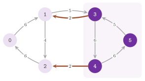
Figure 15.1 has, as its minimum cut with node 0 inside, the set \(\{0,1,2\}\),
of value 5, whereas its minimum cut is \(X=\{3,4,5\}\), of value 4, which only
the second phase finds. The program manual/examples/15-hao-orlin.cc (the
test manual_15_hao_orlin) runs the two phases one at a time from node 0 on
this digraph, and then run(). It checks each value against the enumeration
of the \(2^6-2\) cuts.
15.3 The Nagamochi-Ibaraki algorithm¶
15.3.1 Maximum adjacency orderings¶
On an undirected graph, Nagamochi and Ibaraki (1992) find \(\lambda(G)\) without any flow, by orderings of the nodes that certify a lower bound on \(\lambda(u,v)\) for many pairs at once. We assume in this section that \(G\) has no loops and no parallel edges (the algorithm merges the parallel edges, and a loop is in no cut), and for a node \(u\) and a set \(B\subseteq V\) we write \(c(u,B)\) for the capacity of the edges between \(u\) and the nodes of \(B\). An ordering \(v_1,\ldots,v_n\) of the nodes is a maximum adjacency ordering if \(v_1\) is arbitrary and each \(v_j\), \(j\geq 2\), maximizes the adjacency \(c(v,V_{j-1})\) among the nodes \(v\notin V_{j-1}\), where \(V_k=\{v_1,\ldots,v_k\}\). For an edge \(e=v_iv_j\) with \(i<j\) we write \(q(e)=c(v_j,V_i)\); this is the adjacency of \(v_j\) just after \(v_i\) has been ordered, i.e., the key of \(v_j\) in the priority queue when \(e\) is scanned. Given a cut \(X\), we call \(v_k\), \(k\geq 2\), active for \(X\) if \(v_{k-1}\) and \(v_k\) lie on different sides of \(X\), and we write \(\delta_k(X)\) for the edges of \(\delta(X)\) with both ends in \(V_k\). The next two lemmas follow the argument of Stoer and Wagner (1997).
Lemma 15.4. In a maximum adjacency ordering, every node \(v_k\) active for a cut \(X\) satisfies \(c(v_k,V_{k-1})\leq c(\delta_k(X))\).
Proof. By induction on the active nodes, in their order. For the first active node \(v_k\), the nodes \(v_1,\ldots,v_{k-1}\) lie on the same side, and \(v_k\) on the other; hence, every edge between \(v_k\) and \(V_{k-1}\) is in \(\delta_k(X)\). Let now \(v_k\) be active and let \(v_a\), \(a<k\), be the previous active node. When \(v_a\) was ordered, \(v_k\) was not yet, and therefore \(c(v_k,V_{a-1})\leq c(v_a,V_{a-1})\leq c(\delta_a(X))\), by the maximality of the ordering and by the induction hypothesis. The nodes \(v_a,\ldots,v_{k-1}\) lie on the same side (there is no active node between \(a\) and \(k\)), and \(v_k\) on the other, since it is active; hence, the edges between \(v_k\) and \(V_{k-1}\setminus V_{a-1}\) are in \(\delta_k(X)\), and they are not in \(\delta_a(X)\), which only has edges inside \(V_a\). Adding up, \(c(v_k,V_{k-1})=c(v_k,V_{a-1})+c(v_k,V_{k-1}\setminus V_{a-1})\leq c(\delta_k(X))\). \(\square\)
Lemma 15.5. In a maximum adjacency ordering, every edge \(e=v_iv_j\) with \(i<j\) satisfies \(\lambda(v_i,v_j)\geq q(e)\). In particular, the edge between \(v_n\) and the node of \(V_{n-1}\) ordered last among its neighbours has \(q(e)=c(\delta(v_n))\).
Proof. Let \(X\) be a cut that separates \(v_i\) from \(v_j\), and let \(v_a,\ldots,v_i\) be the longest run of consecutive nodes of the ordering that ends at \(v_i\) and lies on the side of \(v_i\). If \(a=1\), all of \(V_i\) lies on the side opposite to \(v_j\), and \(q(e)=c(v_j,V_i)\leq c(\delta(X))\). Otherwise \(v_a\) is active, and \(v_j\) was not yet ordered when \(v_a\) was; hence, by the maximality of the ordering and by Lemma 15.4, \(c(v_j,V_{a-1})\leq c(v_a,V_{a-1})\leq c(\delta_a(X))\). The edges between \(v_j\) and \(v_a,\ldots,v_i\) are in \(\delta(X)\) and not in \(\delta_a(X)\), since \(v_j\notin V_a\); adding up, \(q(e)=c(v_j,V_{a-1})+c(v_j,V_i\setminus V_{a-1})\leq c(\delta(X))\). Since \(X\) is arbitrary, \(\lambda(v_i,v_j)\geq q(e)\). For the second part, the key of \(v_n\) after the last of its neighbours has been ordered is \(c(v_n,V_{n-1})\), which is \(c(\delta(v_n))\). \(\square\)
It follows that an edge with \(q(e)\) not smaller than the value \(\mu\) of a cut already found can be contracted: a cut that separates its ends has capacity at least \(\lambda(v_i,v_j)\geq q(e)\geq\mu\), and it is not better than the one at hand. Each phase of the algorithm computes one ordering and takes as \(\mu\) the least capacity of a prefix \(V_k\), \(1\leq k<n\), of the ordering (these are cuts, and their capacities are computed while the ordering is built, by \(c(\delta(V_k))=c(\delta(V_{k-1}))+c(\delta(v_k))-2c(v_k,V_{k-1})\)). Then it contracts the edges with \(q(e)\geq\mu\), i.e., it merges their two ends into one node, merges the parallel edges so created by adding their capacities, and drops the loops.
Algorithm 15.2 (Nagamochi-Ibaraki).
 1  skip the loops and merge the parallel edges;
    lambda <- min_v c(delta(v)); X <- that {v}
 2  if lambda = 0: stop
 3  repeat
 4    build a maximum adjacency ordering v_1, ..., v_n' of the current
      nodes from the first one, with q(e) for every edge e
 5    if it does not reach every node: X <- the original nodes of
      the nodes reached; lambda <- 0; stop
 6    mu <- min{ c(delta(V_k)) : 1 <= k < n' }, attained at V_k
 7    if mu < lambda: lambda <- mu; X <- the original nodes of V_k
 8    contract the edges e with q(e) >= mu
 9  until a single node is left
In the class, steps 1 and 2 are init(), and steps 4 to 9 are one call of
processNextPhase(). In lemon/nagamochi_ibaraki.h the keys of the ordering
are kept in a heap that maximizes them, and the value \(q(e)\) is stored on the
edge (cut) when it is scanned. The original nodes merged into a node are
kept in a linked list (_next_rep), which steps 5 and 7 follow to write the
cut. Step 5 detects a disconnected graph, whose cut of value 0 is the
connected component of the first node. Step 8 scans the edges of each current
node, and the edges of a node merged into it are appended to its list, so that
they are scanned in the same step. An edge built by merging two parallel edges
keeps the larger of their two values \(q\). In abLEMON the comparisons of steps
1, 2 and 7 go through the tolerance, while those of steps 6 and 8 are exact.
Theorem 15.5. With exact comparisons, Algorithm 15.2 applied to a graph with at least two nodes terminates after at most \(n-1\) phases, and at the end \(X\) is a minimum cut of \(G\) and \(\lambda=\lambda(G)\).
Proof. Each cut of the current graph, expanded to the original nodes merged into its nodes, is a cut of \(G\) of the same capacity, since the merged parallel edges carry the sum of the capacities and the dropped loops join nodes of the same side. We show that after each step the stored \(X\) is a cut of \(G\) of capacity \(\lambda\). We also show that either \(\lambda=\lambda(G)\) or a minimum cut of \(G\) is still a cut of the current graph, i.e., separates no two original nodes merged into one node. This holds after step 1, where nothing has been merged, and at the stop of step 2, since no cut has a negative capacity. If step 5 stops, the nodes reached form a union of connected components of the current graph, i.e., a cut of value 0, which is minimum. After step 7 one has \(\lambda\leq\mu\); at step 8, by Lemma 15.5, every cut of the current graph that separates the ends of a contracted edge has capacity at least \(q(e)\geq\mu\geq\lambda\). This also holds for an edge that step 8 builds from two parallel edges \(vu\) and \(wu\) after merging \(v\) and \(w\), with the larger of their values \(q\): a cut that does not separate \(v\) from \(w\) but separates them from \(u\) separates both pairs. Hence, if a minimum cut of \(G\) of value less than \(\lambda\) was a cut of the current graph, it separates the ends of no contracted edge and remains a cut of the contracted graph; otherwise \(\lambda=\lambda(G)\). When a single node is left, no cut of \(G\) is a cut of the current graph, and therefore \(\lambda=\lambda(G)\). Finally, at step 6 the prefix \(V_{n'-1}\) has \(c(\delta(V_{n'-1}))=c(\delta(v_{n'}))\), and hence \(\mu\leq c(\delta(v_{n'}))\). By Lemma 15.5 the last edge scanned into \(v_{n'}\) has \(q(e)=c(\delta(v_{n'}))\geq\mu\); since step 8 scans every current edge, at least one edge is contracted in each phase, which merges two nodes. \(\square\)
Theorem 15.6. init() runs in \(O(n+m)\) time,
and a phase in \(O(m\log n)\) time with the default binary heap and in
\(O(m+n\log n)\) time with a Fibonacci heap; hence, run() takes
\(O(nm\log n)\) and \(O(nm+n^2\log n)\) time, respectively.
Proof. Step 1 scans each edge from its two ends once, and the parallel edges
are found by remembering, for each neighbour of the node being scanned, the
last edge built towards it (curr_arc). A phase inserts and removes each
current node once in the heap, and increases the key of a node once for each
edge scanned, i.e., at most \(m\) times. With a binary heap each of these
operations costs \(O(\log n)\), and with a Fibonacci heap the \(n\) removals cost
\(O(\log n)\) amortized each and the increases \(O(1)\) amortized each
(chapter 7). Steps 5 to 7 cost \(O(n)\), and step 8 handles
each edge of a merged node once, in \(O(m)\). By Theorem 15.5 there are at most
\(n-1\) phases. \(\square\)
The header adds that with unit capacities a bucket heap gives \(O(nm)\). We remark, however, that the merged edges no longer have unit capacities. Also, the test of the library runs only the binary heap and the Fibonacci heap.
15.3.2 The class NagamochiIbaraki¶
The class is declared as
template< typename GR , typename CM = typename GR::template EdgeMap< int > , typename TR = NagamochiIbarakiDefaultTraits< GR , CM > > class NagamochiIbaraki,
where GR is an undirected graph type, CM a readable edge map of
capacities, and TR the traits class. Its public types are Traits, Graph,
CapacityMap, Value (the value type of the capacities), Heap and
HeapCrossRef, and Create, the class itself, as in every class with named
template parameters (chapter 3). The default traits
NagamochiIbarakiDefaultTraits< GR , CM > define Value, Graph,
CapacityMap, the cross reference HeapCrossRef (i.e.,
GR::NodeMap< int >), the heap
BinHeap< Value , HeapCrossRef , std::greater< Value > >, a binary heap that
maximizes the keys, and the functions that allocate them:
createCapacityMap( graph ), which fails with an assertion (the capacities
must be given to the constructor), createHeapCrossRef( graph ) and
createHeap( crossref ).
There are two constructors: NagamochiIbaraki( graph , capacity ) takes the
graph and the capacities, while NagamochiIbaraki( graph ) is meant for the
named template parameter SetUnitCapacity, whose traits allocate a constant
map of value 1 on the edges; e.g.,
NagamochiIbaraki< G >::SetUnitCapacity::Create ni( g ) computes the edge
connectivity of g. Furthermore, the class declares the named parameters
SetHeap< H , CR > and SetStandardHeap< H , CR >, where H is a heap that
maximizes the keys and CR its cross reference, a node map of int by
default. With SetStandardHeap the algorithm constructs the cross reference
on the graph and the heap on the cross reference, while with SetHeap they
must be handed to the algorithm by heap( hp , cr ) before init()
(otherwise init() fails with an assertion). The function heap( hp , cr )
takes objects of the types Heap and HeapCrossRef of the class, and it may
also be used with the other traits, in which case the class uses the given
objects instead of allocating its own. For instance, a Fibonacci heap of
std::greater< Value > gives the bounds of the second case of Theorem 15.6.
abLEMON
In LEMON 1.3.1 the two named parameters did not compile, since the
function that allocates the structures passes the graph to the
createHeapCrossRef() of their traits, which took an int, and their
default cross reference was a RangeMap< int >; the test
nagamochi_ibaraki_test now runs both with a Fibonacci heap. In LEMON
1.3.1 step 8 gave the larger value \(q\) of two merged parallel edges to the
edge it dropped rather than to the one it kept, which could leave the
latter uncontracted until a later phase; nagamochi_ibaraki_test checks a
graph that a single phase contracts. LEMON 1.3.1 did not state that the
graph must not be empty, and on an empty graph init() wrote the cut map
at the node INVALID; since this is a precondition, no test checks it,
while edge_case_test checks the graphs of one node.
In the execution, init() builds the internal copy of the graph and makes
steps 1 and 2. Then processNextPhase() makes one phase and returns true
when the algorithm has finished (and again at every later call), start()
calls it until then, and run() is init() followed by start();
tolerance( tol ) and tolerance() set and read the Tolerance< Value > of
the comparisons. As for the results, minCutValue() returns the value of the
best cut found so far, which after init() is already the capacity of a cut
(the lightest star of a node) and at the end is \(\lambda(G)\) by Theorem 15.5.
Similarly, minCutMap( cutMap ) writes the characteristic vector of one side
of that cut into a writable bool node map, and returns its value. The graph
must have at least one node, which init() asserts; a graph of one node has
no cut, and the class then gives the value 0 and the set of that node. Also,
the header warns that the value type must hold the cut values of the graph,
since their sums may otherwise overflow, and notes that the capacities are
supposed to be integer. With floating-point capacities the result rests on the
tolerance and on the exact comparisons of steps 6 and 8, and the tests of the
library cover only integer capacities. On the graph of Figure 15.2 the
algorithm finds the value 3 (section 15.4.2 names the program that runs it
phase by phase).
abLEMON
tolerance() is new in abLEMON. LEMON 1.3.1 compared the cut values
exactly, whereas abLEMON compares through the tolerance the stars of step
1, the value 0 that ends step 2, and the update of step 7.
15.4 Gomory-Hu trees¶
15.4.1 The construction¶
Gomory and Hu's original construction (Gomory and Hu
1961) computes \(n-1\) maximum flows on
graphs obtained by contracting parts of \(G\). Gusfield
(1990) showed that a tree with the
properties of Theorem 15.2 can be obtained by \(n-1\) maximum flows on the
original graph, if the cuts are kept in a rooted tree that is rearranged after
each flow. This second construction is the one of lemon/gomory_hu.h; there
each node \(v\) other than the root \(r\) has a parent \(p(v)\) and a weight \(w(v)\),
the weight of the edge \(v\,p(v)\) of the tree, and the nodes are processed in
the order of the node iterator.
Algorithm 15.3 (Gomory-Hu tree, the construction of Gusfield).
 1  r <- the first node; p(v) <- r for every v != r
 2  for each node v != r, in the order of the node iterator:
 3    compute a minimum cut X between v and p(v), v in X, and its
      value f, by Preflow on G
 4    w(v) <- f
 5    for each u != v with u in X and p(u) = p(v): p(u) <- v
 6    if p(p(v)) is defined and lies in X:
 7      u <- p(v); p(v) <- p(u); p(u) <- v; w(v) <- w(u); w(u) <- f
 8  number the nodes so that every node comes after its parent
Step 3 is a call of Preflow::runMinCut() with the tolerance of the class,
and \(X\) is the source side given by minCut(). Step 7 makes \(v\) the parent of
its former parent when the cut puts its grandparent on its side: \(v\) takes the
place of \(p(v)\) under the grandparent, with the weight that \(p(v)\) had, and
\(p(v)\) hangs from \(v\) with the weight \(f\). Step 8 computes the numbering by
which the queries climb the two paths of the tree towards their common
ancestor. The correctness of the construction rests on the fact that minimum
cuts can be chosen so that they do not cross. We state it for the cut
function \(\kappa(Y)=c(\delta(Y))\) of \(G\). We recall that it is submodular,
i.e., \(\kappa(Y)+\kappa(Z)\geq\kappa(Y\cap Z)+\kappa(Y\cup Z)\) for any two
sets \(Y\) and \(Z\) (an edge counted on the right is counted at least as many
times on the left).
Lemma 15.6. Let \(X\) be a minimum \(s\)-\(t\) cut of \(G\), and let \(u\neq v\) be two nodes of \(X\). Then there is a minimum cut between \(u\) and \(v\) contained in \(X\).
Proof. Let \(Y\) be a minimum \(u\)-\(v\) cut. If \(t\in Y\), we replace \(Y\) by \(V\setminus Y\), which by the symmetry of \(\kappa\) is a minimum \(v\)-\(u\) cut, and in both cases \(t\notin Y\) and \(Y\) contains one of \(u\) and \(v\) but not the other. Then \(X\cap Y\) separates \(u\) from \(v\) and is contained in \(X\), while \(X\cup Y\) contains \(s\) and not \(t\), and therefore \(\kappa(X\cup Y)\geq\kappa(X)\). By submodularity, \(\kappa(X\cap Y)\leq\kappa(X)+\kappa(Y)-\kappa(X\cup Y)\leq\kappa(Y)\), i.e., \(X\cap Y\) is a minimum cut between \(u\) and \(v\). \(\square\)
Theorem 15.7. At the end of Algorithm 15.3, for every node \(v\neq r\) the nodes of the subtree of \(v\) in the tree of the parents form a minimum \(v\)-\(p(v)\) cut of \(G\), of capacity \(w(v)\); hence, by the proof of Theorem 15.2, the tree with the edges \(v\,p(v)\) and the weights \(w(v)\) is a Gomory-Hu tree.
Proof sketch. This is the theorem of Gusfield (1990) on his cut-tree method, and the proof is an induction on the iterations of step 2. After the iteration of \(v\), every processed node \(u\) has \(w(u)=\lambda(u,p(u))\), and the cuts that the processed nodes have produced can be taken pairwise non-crossing. The induction step rests on Lemma 15.6, which shows that the minimum cut of step 3 can be taken so that it does not cross those of the nodes processed before. Steps 5 and 7 then rearrange the tree so that each subtree is the side of the cut of its root. The details, and the proof that the arbitrary minimum cut returned by the maximum flow is enough, are in Gusfield (1990); the Gomory-Hu theorem, with the uncrossing of Lemma 15.6, is also in Schrijver (2003), §15.4. \(\square\)
The queries of the class climb the tree with the numbering of step 8, which we call \(o(v)\) (it is \(0\) for the root, and larger for a node than for its parent), and the next lemma shows that the climb meets the common ancestor.
Lemma 15.7. Consider the procedure that starts from two nodes \(s\) and \(t\) and, while the two current nodes differ, replaces the one of larger number \(o\) by its parent. It stops at the nearest common ancestor \(a\) of \(s\) and \(t\), after \(h(s)+h(t)-2h(a)\) steps, where \(h\) is the depth in the tree, and the edges that it climbs form the path of the tree from \(s\) to \(t\).
Proof. If the current nodes \(x\neq y\) have \(o(x)<o(y)\), then \(y\) is not an ancestor of \(x\), since an ancestor has a smaller number. Hence, the nearest common ancestor of \(x\) and \(y\) is a proper ancestor of \(y\), and it does not change when \(y\) is replaced by its parent. Each step decreases \(h(x)+h(y)\) by one, and the procedure stops when \(x=y\), i.e., at the common ancestor; the edges climbed are those from \(s\) and from \(t\) up to it. \(\square\)
Theorem 15.8. run() takes the time of \(n-1\)
calls of Preflow::runMinCut() plus \(O(n^2)\), i.e., \(O(n^3m\Delta)\). Let \(h\)
be the height of the tree. Then minCutValue( s , t ) takes \(O(h)\) time, and
minCutMap( s , t , cutMap ) and the constructors of the two iterators take
\(O(n)\) time.
Proof. Steps 5 to 7 scan the nodes once per iteration, in \(O(n)\), and step 8
climbs from each node to the first numbered ancestor and numbers the nodes on
the way, in \(O(n)\) in all. Each first phase of Preflow costs
\(O(n^2m\Delta)\), \(\Delta\) being the largest degree of a node, by
Theorem 12.3 (the bound \(O(n^2\sqrt{m})\) of the
highest label rule needs a current arc for each node, which Preflow does
not keep). By Lemma 15.7
minCutValue() makes at most \(2h\) steps. Then minCutMap() finds the
lightest edge of the path in the same way, in \(O(h)\), and writes the side of
each node by climbing from it to the first node whose side is known, the root
and the lower end of that edge being known from the start. Since every node
climbed through is marked when its side is written, each node is climbed
through once, and the \(n\) climbs cost \(O(n)\) in all, as does the map of the
marks; since \(h<n\), the bound is \(O(n)\). \(\square\)
15.4.2 The class GomoryHu¶
The class is declared as
template< typename GR , typename CAP = typename GR::template EdgeMap< int > > class GomoryHu,
where GR is an undirected graph type and CAP a readable edge map of
capacities (the constructor checks the ReadMap concept on it). Its public
types are Graph, Capacity and Value, and it has no traits class. Its
constructor GomoryHu( graph , capacity ) stores the references,
tolerance( tol ) and tolerance() set and read the Tolerance< Value >
given to the maximum flows, and run() executes Algorithm 15.3 (there is no
public init()). One reads the tree by predNode( v ), the parent of \(v\)
(INVALID for the root), and by predValue( v ), the weight of the edge
between \(v\) and its parent (undefined for the root, where it is in fact the
largest value of Value). Also, rootDist( v ) returns the number \(o(v)\) of
step 8: \(0\) for the root, and for any other node a number larger than that of
its parent, distinct for distinct nodes, i.e., an order of the tree from the
root, not the distance from it.
A minimum cut between two nodes is read by minCutValue( s , t ), which
climbs the two paths of the tree to their common ancestor and returns the
least weight met (Lemma 15.7 and Theorem 15.2). In the same way
minCutMap( s , t , cutMap ) finds the lightest edge of the path, writes
true on the side of \(s\) and false on the other side into a readable and
writable bool node map, and returns the value. For \(s=t\), which no cut
separates, both return the largest value of Value, and minCutMap() writes
true at every node, so that the iterators below list every node on the side
of \(s\) and no edge. A cut can also be listed by two iterators.
MinCutNodeIt( gomory , s , t , side = true ) lists the nodes of the side of
\(s\) (or those of the other side if side is false). Similarly,
MinCutEdgeIt( gomory , s , t , side = true ) lists the edges of the cut,
each once, as the arc that leaves the side of \(s\) (or enters it if side is
false); the latter converts to both Arc and Edge. Each constructor calls
minCutMap() on a node map that the iterator holds, at the cost of Theorem
15.8, and the postfix increments return a Node (respectively an Arc)
instead of an iterator. Since a minimum cut need not be unique,
MinCutNodeIt( gomory , s , t , true ) and
MinCutNodeIt( gomory , t , s , false ) may list different nodes, whereas
MinCutNodeIt( gomory , s , t , true ) and
MinCutNodeIt( gomory , s , t , false ) together list each node once. On an
empty graph run() builds an empty tree.
abLEMON
tolerance() is new in abLEMON. LEMON 1.3.1 gave its maximum flows the
default tolerance of the value type, while abLEMON gives them the one set
on the class. In LEMON 1.3.1 minCutMap() did not mark the nodes it
climbed through, and took \(O(nh)\) time; for \(s=t\) it wrote the maps at
the node INVALID, as run() did on an empty graph. The test
gomory_hu_test counts the writes of minCutMap() on a path, and checks
\(s=t\) and the graphs of zero and one node.
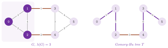
On the graph of Figure 15.2 the tree is the path \(0,1,2,4,3,5\) with the
weights \(5,7,3,6,6\); hence, e.g., \(\lambda(0,5)=3\) and \(\lambda(1,2)=7\). The
program manual/examples/15-undirected-cuts.cc (the test
manual_15_undirected_cuts) computes the minimum cut of this graph by
NagamochiIbaraki, one phase at a time, and then its Gomory-Hu tree. It
checks the value of the cut against the enumeration of all the cuts. For each
of the 15 pairs of nodes, it also checks the value read from the tree against
a maximum flow, the sides given by minCutMap(), and the sum of the
capacities listed by MinCutEdgeIt.
15.5 Choosing an algorithm¶
For a digraph HaoOrlin is the only class of the chapter, and it is arguably
also the natural choice when one needs the best cut on a given side of a node
(the stored cut after calculateOut()). For the minimum cut of an undirected
graph, NagamochiIbaraki uses no flow, and its phases may be far fewer than
\(n-1\), since all the edges with \(q(e)\geq\mu\) are contracted at once. On the
other hand, HaoOrlin with the first phase only, on the Undirector, has the
bound of a single maximum flow (Theorem 15.4), against the \(O(nm\log n)\) of
Theorem 15.6. Which of the two is faster typically depends on the instance,
and neither the headers nor the works cited here give a rule that settles it
in general. GomoryHu costs \(n-1\) maximum flows. It pays off when the cuts of
"many" pairs of nodes are needed, since each value is then read from the tree
in \(O(h)\) time, whereas for the cut of one pair (or of a "few" pairs) a
maximum flow of chapter 12 is cheaper.
15.6 Exercises¶
Exercise 15.1. Check Theorem 15.1 on the
digraph of Figure 15.1 by computing \(\lambda(0,t)\) and \(\lambda(t,0)\) with
Preflow for every \(t\neq 0\) and comparing the least of them with
HaoOrlin::minCutValue() (the program manual/examples/15-hao-orlin.cc gives
the value 4).
Exercise 15.2. Show that, on the digraph
Undirector< GR > of an undirected graph, the value stored after
calculateOut() is already \(\lambda(G)\), and verify it on the graph of
test/hao_orlin_test.cc, whose test runs both phases.
Exercise 15.3. Compute the edge connectivity of
the graph of Figure 15.2 with
NagamochiIbaraki< SmartGraph >::SetUnitCapacity::Create, and check the cut
it gives by counting its edges (the fourth block of
test/nagamochi_ibaraki_test.cc does the same on another graph).
Exercise 15.4. Print the value minCutValue()
of NagamochiIbaraki on the graph of Figure 15.2 after init() and after
each call of processNextPhase(). Explain why the sequence is nonincreasing,
and why its first value is the lightest star of a node (5, at node 0).
Exercise 15.5. Using only predNode() and
predValue() of GomoryHu, count the distinct values among the
\(\lambda(s,t)\) of a graph, and deduce from Theorem 15.2 that there are at most
\(n-1\) of them; check the values against minCutValue( s , t ) for each pair,
as test/gomory_hu_test.cc does against Preflow.
Exercise 15.6. Show that the sum of the
capacities listed by MinCutEdgeIt( gomory , s , t ) equals
minCutValue( s , t ), and that the nodes listed by MinCutNodeIt with
side true and false partition \(V\) (both facts are checked by
test/gomory_hu_test.cc, the first also by
manual/examples/15-undirected-cuts.cc).