16. Minimum mean cycles
We are concerned in this chapter with the directed cycles of least mean cost
of a digraph, i.e., with the cycles whose cost divided by their number of arcs
is minimum. abLEMON has three algorithms for this problem, in the group
Minimum Mean Cycle
Algorithms:
Karp's algorithm (KarpMmc, in lemon/karp_mmc.h), its variant with early
termination by Hartmann and Orlin (HartmannOrlinMmc, in
lemon/hartmann_orlin_mmc.h), and Howard's policy iteration (HowardMmc, in
lemon/howard_mmc.h). All three have the same interface, stated as the
concept concepts::MinMeanCycle of lemon/concepts/min_mean_cycle.h. Inside
the library, the minimum mean cycle is used by the cycle-canceling algorithm
of chapter 13 and by the certificates of
unboundedness of chapter 14. Section 16.1 states
the problem and its optimality conditions, and sections 16.2 to 16.4 describe
the three algorithms with their proofs; section 16.5 describes the interface
they share, and section 16.6 has the exercises.
16.1 The problem
Let \(D=(V,A)\) be a digraph with \(n\) nodes, \(m\) arcs and a cost \(c(a)\in\mathbb{R}\) on each arc \(a\). A walk is a sequence of arcs in which each arc starts where the previous one ends, and it is closed if the last arc ends where the first one starts; a directed cycle is a closed walk that visits no node twice. A closed walk \(W\) has \(|W|\) arcs (counted with their repetitions) and cost \(c(W)=\sum_{a\in W}c(a)\), and its mean cost is \(\mu(W)=c(W)/|W|\). The minimum cycle mean of \(D\) is
A digraph without directed cycles has no minimum cycle mean, and the algorithms report this case. This problem is closely related to conservative costs, i.e., to costs under which no directed cycle has a negative cost (cf. Ahuja, Magnanti and Orlin 1993, chapter 5). We first collect the elementary facts that the proofs of this chapter use.
Lemma 16.1. (i) A closed walk \(W\) is the union of directed cycles \(C_1,\ldots,C_p\) (possibly with repetitions), and \(\min_i\mu(C_i)\leq\mu(W)\leq\max_i\mu(C_i)\); in particular, \(\mu(W)\geq\mu^*(D)\), and if \(\mu(W)=\mu^*(D)\) then each \(C_i\) is a minimum mean cycle. (ii) Adding a constant \(\alpha\) to the cost of all the arcs adds \(\alpha\) to the mean of each closed walk, and hence it leaves the minimum mean cycles unchanged. (iii) A directed cycle lies in one strongly connected component of \(D\), and therefore \(\mu^*(D)\) is the least of the minimum cycle means of the components that have a cycle.
Proof. (i) If \(W\) visits no node twice (except at its end), it is a cycle. Otherwise, we take two visits of the same node with no repeated node between them: the arcs between them form a cycle \(C_1\), and removing them leaves a shorter closed walk, to which we apply induction. Then \(c(W)=\sum_i c(C_i)\) and \(|W|=\sum_i|C_i|\), and \(\mu(W)\) is the average of the \(\mu(C_i)\) with weights \(|C_i|/|W|\), which lies between their minimum and their maximum. If it equals \(\mu^*(D)\), which is a lower bound on each \(\mu(C_i)\), all of them equal it. (ii) \(c(W)+\alpha|W|\) divided by \(|W|\) is \(\mu(W)+\alpha\). (iii) The nodes of a cycle are mutually reachable. \(\square\)
The algorithms of this chapter use (iii) as it stands. They find the strongly
connected components first, by stronglyConnectedComponents() of chapter
18, solve the problem on each component that has a
cycle (i.e., on each component of at least two nodes, and on each node with a
loop), and keep the best cycle. The optimality condition is the following one.
Theorem 16.1. Let \(\mu\in\mathbb{R}\). Each directed cycle of \(D\) has mean cost at least \(\mu\) if and only if there are potentials \(\pi:V\rightarrow\mathbb{R}\) such that
Proof. If (16.2) holds, summing it along a cycle \(C\) cancels the potentials and gives \(c(C)-\mu|C|\geq 0\), i.e., \(\mu(C)\geq\mu\). Conversely, if no cycle has mean less than \(\mu\), the costs \(c'=c-\mu\) give no cycle a negative cost. We add a node \(r\) and an arc of cost 0 from \(r\) to each node, and we let \(\pi(v)\) be the least \(c'\)-cost of a walk from \(r\) to \(v\). This value is finite, since removing the cycles of a walk (Lemma 16.1 (i)) does not increase its cost, and the least is therefore taken over the finitely many paths. Since a walk to \(u\) followed by \((u,v)\) is a walk to \(v\), one has \(\pi(v)\leq\pi(u)+c(u,v)-\mu\), which is (16.2). \(\square\)
Hence, \(\mu^*(D)\) is the largest \(\mu\) for which the costs \(c-\mu\) are conservative, i.e., the negative of the smallest amount that, added uniformly to the costs, makes them conservative (as the documentation of the group puts it). Furthermore, a closed walk \(W\) together with potentials that satisfy (16.2) for \(\mu=\mu(W)\) certifies, by Theorem 16.1 and Lemma 16.1 (i), that \(\mu(W)=\mu^*(D)\) and that the cycles of \(W\) are minimum mean cycles. Hartmann and Orlin check a certificate of this kind to stop early, and Howard's algorithm stops when its distances (section 16.4) are such a certificate.
16.2 Karp's algorithm
Let \(D\) be strongly connected and have a cycle, and let \(s\) be any node. For \(k=0,\ldots,n\) and \(v\in V\), let \(D_k(v)\) be the least cost of a walk from \(s\) to \(v\) with exactly \(k\) arcs (\(+\infty\) if there is none). Then \(D_0(s)=0\), \(D_0(v)=+\infty\) for \(v\neq s\), and
since the last arc of a walk of \(k\) arcs to \(v\) enters \(v\) from a node reached by a walk of \(k-1\) arcs. Each node has an arc leaving it inside \(D\) (it lies on a cycle), and hence walks of any length start at \(s\); in particular, \(D_n(v)<\infty\) for some \(v\). We use the following characterization, due to Karp (1978).
Theorem 16.2. If \(D\) is strongly connected and has a cycle, then
Furthermore, if \(v^*\) attains the minimum, a walk of \(n\) arcs from \(s\) to \(v^*\) of cost \(D_n(v^*)\) visits some node twice, and the arcs between two visits of a node with no repeated node between them form a cycle of mean \(\mu^*(D)\).
Proof. Let \(\mu^*=\mu^*(D)\). Subtracting \(\mu^*\) from the costs changes \(D_k(v)\) into \(D_k(v)-k\mu^*\), and hence each ratio of (16.4) into the ratio minus \(\mu^*\), while it leaves the walks that attain the values and (by Lemma 16.1 (ii)) the minimum mean cycles unchanged. We may therefore assume \(\mu^*=0\), i.e., that no cycle is negative and some cycle \(C\) has cost 0, and we must show that the right-hand side of (16.4) is 0. Let \(\delta(v)\) be the least cost of a walk from \(s\) to \(v\) of any length; as in the proof of Theorem 16.1, it is attained by a path, which has fewer than \(n\) arcs, and hence \(\delta(v)=\min_{0\leq k<n}D_k(v)\). If \(D_n(v)<\infty\), then \(D_n(v)\geq\delta(v)\), and the inner maximum at \(v\), which is at least \((D_n(v)-\delta(v))/(n-k)\) for the \(k\) that attains \(\delta(v)\), is nonnegative.
To see that some \(v\) gives 0, let \(w\) be a node of \(C\) and \(P\) a path from \(s\) to \(w\) of cost \(\delta(w)\), and, for two nodes \(x,y\) of \(C\), let \(c_C(x,y)\) be the cost of the arcs of \(C\) from \(x\) to \(y\). Since \(\delta(y)\leq\delta(x)+c_C(x,y)\), \(\delta(x)\leq\delta(y)+c_C(y,x)\) and \(c_C(x,y)+c_C(y,x)=c(C)=0\), one has \(\delta(y)=\delta(w)+c_C(w,y)\) for each node \(y\) of \(C\). We follow \(P\) and then \(C\) until the walk has \(n\) arcs (which is possible, since \(|P|<n\)), and we let \(v\) be its last node. The cost of this walk is \(\delta(w)+c_C(w,v)=\delta(v)\), which gives \(D_n(v)\leq\delta(v)\), and hence \(D_n(v)=\delta(v)\). The inner maximum at \(v\) is then at most 0, since \(D_k(v)\geq\delta(v)=D_n(v)\) for all \(k\), and therefore it is 0.
For the second claim, the minimizer \(v^*\) has inner maximum 0, which gives, by the same two inequalities, \(D_n(v^*)=\delta(v^*)\). A walk \(W\) of \(n\) arcs has \(n+1\) visits of nodes, and hence some node repeats. Removing from \(W\) its cycles, one at a time, as in Lemma 16.1 (i), leaves a path from \(s\) to \(v^*\) of cost at least \(\delta(v^*)\), and the removed cycles have nonnegative costs. Since the total is \(c(W)=\delta(v^*)\), each removed cycle has cost \(0=\mu^*\), and the cycle between the two visits of the statement may be taken as the first one removed. \(\square\)
Karp's algorithm computes the table (16.3) round by round and then evaluates
(16.4). In KarpMmc this is done on each strongly connected component that
has a cycle, with \(s\) its first node and \(n\) its number of nodes. In the last
step, the walk back reads, at each node \(v\) and round \(k\), the arc
\(\mathrm{pred}_k(v)\) through which \(D_k(v)\) was last improved.
Algorithm 16.1 (Karp, on a strongly connected component of n nodes).
1  s <- the first node; D_0(s) <- 0; D_j(v) <- +inf for all other (v, j)
2  R <- { s }                              (the nodes with D_{k-1} < +inf)
3  for k = 1, ..., n:
4    for each node u of R (of the component, once R has all n nodes):
5      for each arc (u, v) of the component:
6        if D_{k-1}(u) + c(u, v) < D_k(v):
7          D_k(v) <- D_{k-1}(u) + c(u, v); pred_k(v) <- (u, v)
8    if R has fewer than n nodes: R <- { v : D_k(v) < +inf }
9  for each node v with D_n(v) < +inf:
10   M(v) <- max{ (D_n(v) - D_k(v)) / (n - k) : 0 <= k < n, D_k(v) < +inf }
11 mu <- min_v M(v), attained at v*               (findCycleMean ends here)
12 (findCycle) walk back from v* along pred_n, pred_{n-1}, ... until a
   node repeats; the arcs between its two visits form the cycle
Steps 4 to 8 are processNextBuildRound() while \(R\) has fewer than \(n\) nodes,
and processNextFullRound() afterwards; the comparison of step 6 goes through
the tolerance. In steps 10 and 11 the ratios are compared without division, by
cross-multiplication in the type LargeCost. The first node (in the order of
the component) that attains the minimum is kept. Across the components, the
best cycle is replaced only by a strictly better one. As the next lemma shows,
the full rounds add no cost to an infinite value.
Lemma 16.2. Steps 3 to 8 of Algorithm 16.1 compute the values (16.3). Furthermore, at each round \(k\) the set \(R\) is the set of the nodes with \(D_{k-1}<\infty\), and once it has all the \(n\) nodes, \(D_j(v)<\infty\) for each \(v\) and each \(j\geq k-1\).
Proof. The minimum (16.3) is over the arcs \((u,v)\) with \(D_{k-1}(u)<\infty\), which are those that step 4 scans while \(R=\{u:D_{k-1}(u)<\infty\}\). The build round collects these nodes as they first get a finite value (a node is added to the next \(R\) when its value for round \(k\) stops being infinite). If \(D_{k-1}(u)<\infty\) for all the nodes \(u\), then \(D_k(v)<\infty\) for all the nodes \(v\), since each node of the component has an arc entering it from the component, and the claim follows by induction on \(k\). \(\square\)
Theorem 16.3. KarpMmc::findCycleMean()
returns false if and only if the digraph has no directed cycle. Otherwise
the mean of the pair it keeps, i.e., cycleCost() divided by cycleSize(),
is \(\mu^*(D)\), and findCycle() then stores a minimum mean cycle in the
path.
Proof. A digraph has a cycle if and only if some strongly connected
component has two nodes or a loop, and these are the components that
initComponent() does not skip. On each of them Lemma 16.2 gives the table
(16.3), and Theorem 16.2 shows that steps 9 to 11 compute the minimum cycle
mean of the component, at the node \(v^*\); by Lemma 16.1 (iii) the best of the
components gives \(\mu^*(D)\). Step 12 follows \(\mathrm{pred}_n(v^*)\),
\(\mathrm{pred}_{n-1}\), and so on, which retrace a walk of \(n\) arcs of cost
\(D_n(v^*)\). It stops at the first repeated node, and by the second part of
Theorem 16.2 its cycle has mean \(\mu^*(D)\). \(\square\)
We remark that until findCycle() has been called, cycleCost() and
cycleSize() return the numerator \(D_n(v^*)-D_k(v^*)\) and the denominator
\(n-k\) of the ratio of (16.4) at \(v^*\). Their quotient is \(\mu^*(D)\), but they
need not be the cost and the length of a cycle; after findCycle(), they are
those of the cycle found in step 12.
Theorem 16.4. Algorithm 16.1 runs in \(O(nm)\) time and \(O(n^2+m)\) space on a digraph of \(n\) nodes and \(m\) arcs.
Proof. The strongly connected components, with their lists of arcs, cost \(O(n+m)\). A component of \(n_i\) nodes has \(m_i\geq n_i\) arcs, since each node has a leaving arc, and each of its \(n_i\) rounds costs \(O(n_i+m_i)\); steps 9 to 11 cost \(O(n_i^2)\) and step 12 costs \(O(n_i)\). The sum over the components is \(O(nm)\). The table of a node of the component \(i\) has \(n_i+1\) entries, which gives \(\sum_i n_i(n_i+1)=O(n^2)\), plus \(O(m)\) for the lists of arcs. \(\square\)
16.3 The Hartmann-Orlin algorithm
Hartmann and Orlin (1993) observed that Karp's table often contains a minimum mean cycle long before round \(n\), and that Theorem 16.1 allows one to recognize it. At some rounds \(k\) the algorithm follows backwards the walks that end at round \(k\), takes the closed walk \(W\) of least mean among those that these walks close, and computes the potentials
Thus, \(\pi(v)\) is \(|W|\) times the least cost under \(c-\mu(W)\) of a walk from \(s\) to \(v\) with at most \(k\) arcs (\(+\infty\) if there is no such walk). If these potentials satisfy (16.2) for \(\mu=\mu(W)\), scaled by \(|W|\), then \(W\) and its cycles are optimal by Theorem 16.1, and the algorithm stops.
Algorithm 16.2 (Hartmann-Orlin, on a strongly connected component of n nodes).
1  as steps 1 to 8 of Algorithm 16.1; after the rounds k = 4, 6, 9, 13,
   ... (each the previous one times 3/2, rounded down) and after k = n:
2    for each node v with D_k(v) < +inf, walk back from v along
     pred_k, pred_{k-1}, ..., pred_1; each time the walk meets again a
     node u, met last at round j' > j, it closes the closed walk of
     cost D_j'(u) - D_j(u) and of j' - j arcs
3    W <- the closed walk of least mean among those closed in step 2,
     with its node u and its round j'
4    if a closed walk was found and k < n:
5      compute pi by (16.5)
6      if pi(v) < +inf for every node v of the component, and
       |W| c(u, v) - c(W) >= pi(v) - pi(u) for every arc (u, v) of
       the component: stop with W
7    if k = n: stop with W
8  (findCycle) walk back from u along pred_j', pred_{j'-1}, ... until a
   node repeats; the arcs between its two visits form the cycle
This schedule of the checks is the one of processRounds() in
lemon/hartmann_orlin_mmc.h, and steps 2 to 7 are checkTermination(); the
comparisons of steps 5 and 6 go through the tolerance, and step 6 first looks
for a node without a potential, then scans the arcs inside the component, the
only ones whose ends have potentials. Across the components, the closed walk
of least mean is kept (the first one, in case of ties), and findCycle()
performs step 8 on it.
abLEMON
In LEMON 1.3.1 step 6 scanned the arcs of the whole digraph, whose ends
outside the component have no potentials computed, and hence the test
could fail more often and delay the stop. It also had no test of the
infinite potentials: with an integer LargeCost, where \(+\infty\) is the
largest value, \(\pi(v)-\pi(u)\) with \(\pi(v)\) infinite and \(\pi(u)<0\)
overflowed, the violated test could pass, and the algorithm could stop
with a closed walk that is not optimal. The test min_mean_cycle_test
checks such an instance, on which LEMON 1.3.1 returned the mean \(89/3\)
instead of \(78/11\).
Theorem 16.5. Assume exact arithmetic. On a strongly connected component with a cycle, Algorithm 16.2 stops with a closed walk \(W\) of mean \(\mu^*\) (the minimum cycle mean of the component), and the cycle of step 8 is a minimum mean cycle.
Proof. The walk back from a node \(v\) at round \(k\) retraces a walk of \(k\) arcs of cost \(D_k(v)\), whose prefix of \(j\) arcs, which ends at a node \(u\), has cost \(D_j(u)\). The arcs between two visits of \(u\) at rounds \(j<j'\) are therefore a closed walk of cost \(D_{j'}(u)-D_j(u)\) and of \(j'-j\) arcs, and by Lemma 16.1 (i) its mean is at least \(\mu^*\). If the algorithm stops in step 6, all the potentials are finite, by its first test. Hence \(\pi/|W|\) satisfies (16.2) for \(\mu=\mu(W)\) on the arcs of the component, and \(\mu(W)\leq\mu^*\) by Theorem 16.1 (applied to the component). If the algorithm stops in step 7, at \(k=n\), the walk back from the node \(v^*\) of Theorem 16.2 closes, at its first repeated node, a cycle of mean \(\mu^*\), and the least mean of step 3 is again at most \(\mu^*\). In both cases \(\mu(W)=\mu^*\). The walk back of step 8 starts where the walk of step 2 met \(u\) at round \(j'\), and it meets a node twice at the latest when it reaches \(u\) again at round \(j\). Hence its cycle consists of arcs of \(W\), and it is one of the cycles of a decomposition of \(W\) as in Lemma 16.1 (i), each of which has mean \(\mu^*\) by that lemma. \(\square\)
Theorem 16.6. Algorithm 16.2 runs in \(O(nm)\) time and \(O(n^2+m)\) space.
Proof. As in Theorem 16.4, the rounds and the table cost \(O(nm)\) and \(O(n^2+m)\). On a component of \(n_i\) nodes and \(m_i\geq n_i\) arcs, the check at round \(k\) walks back \(k\) arcs from at most \(n_i\) nodes, computes (16.5) in \(O(n_ik)\) and scans \(O(m_i)\) arcs. The rounds of the checks grow geometrically, with ratio \(3/2\), up to \(n_i\), plus the check at \(n_i\); hence their sum is \(O(n_i)\) and their number \(O(\log n_i)\). The checks therefore cost \(O(n_i^2+m_i\log n_i)\), which is \(O(n_im_i)\). \(\square\)
In the worst case the checks add to the work of Karp's algorithm, and the
bounds are the same; according to the header, the early termination makes the
algorithm significantly faster on some instances, but slower on others.
Unlike those of KarpMmc, the values of cycleCost() and cycleSize()
after findCycleMean() alone are the cost and the number of arcs of the
closed walk \(W\), which may visit a node more than twice. After findCycle(),
they are those of the cycle of step 8, of the same mean.
16.4 Howard's policy iteration
Howard's algorithm comes from the policy iteration of Markov decision processes (Howard 1960); its use for the minimum mean cycle is analysed in Cochet-Terrasson et al. (1998) and in Dasdan and Gupta (1998). A policy \(p\) chooses one leaving arc \(p(u)\) for each node \(u\) of a strongly connected component, and the arcs chosen form the policy graph, in which every node has out-degree 1. Following the policy from any node one meets a node twice, and hence each node leads to a cycle of the policy graph. Each iteration evaluates the policy by the cycle \(C\) of least mean among them, with \(\lambda=\mu(C)\), and computes the distances \(d\) towards \(C\) under the costs \(w(u,v)=|C|\,c(u,v)-c(C)=|C|\,(c(u,v)-\lambda)\), which are scaled by \(|C|\) to keep integer costs integer; then it improves the policy by these distances.
Algorithm 16.3 (Howard, on a strongly connected component).
1  for each node u: p(u) <- an arc (u, v) of least cost
2  loop
3    find the cycles of the policy graph; C <- the one of least mean,
     v0 <- the first node of C met, or the v0 of the previous iteration
     if it lies on a cycle of the same least mean (then C is that cycle)
4    d(v0) <- 0; backwards from v0 along the policy arcs (u, v),
     breadth-first: d(u) <- d(v) + w(u, v)
5    backwards, breadth-first, from the nodes reached, along any arc
     (u, v) with u not reached: p(u) <- (u, v); d(u) <- d(v) + w(u, v)
6    improved <- false
7    for each arc (u, v): if d(v) + w(u, v) < d(u):
8      d(u) <- d(v) + w(u, v); p(u) <- (u, v); improved <- true
9    if not improved: return C
Steps 1, 3 and 4 to 9 are buildPolicyGraph(), findPolicyCycle() and
computeNodeDistances() of lemon/howard_mmc.h, and each pass of the loop is
one iteration. In step 3 the nodes are taken in the order of the component,
each one followed along the policy until a node already met, and \(C\) is
replaced only by a cycle of strictly smaller mean (compared by
cross-multiplication), or of the same mean if it contains the root of the
previous iteration. The test of step 7 goes through the tolerance, and the
updates of step 8 are made in place, i.e., an arc scanned later reads the
distances already decreased; step 1 compares the costs exactly.
Lemma 16.3. After step 5 of an iteration, all the nodes of the component have a distance, the policy graph consists of the cycle \(C\) and of arcs that lead to it, and \(d(u)=d(v)+w(u,v)\) for each policy arc \((u,v)=p(u)\), that of \(v_0\) included.
Proof. Step 4 reaches the nodes whose policy leads to \(v_0\), among which are those of \(C\), and step 5 reaches all the others, since in a strongly connected component each node has a path to the nodes reached. Each node \(u\) gets its distance from the arc \(p(u)\) that reaches it, which leads to an already reached node, and hence to \(C\). The equality holds by construction for \(u\neq v_0\), and for \(v_0\) because the sum of \(w\) along \(C\) is \(|C|c(C)-|C|c(C)=0\). \(\square\)
Theorem 16.7. Let \(C\) be the cycle of an iteration and \(C'\) the cycle of the next one. Then \(\mu(C')\leq\mu(C)\). Furthermore, if step 7 improves no distance (and the comparisons are exact), \(C\) is a minimum mean cycle of the component.
Proof. Let \(d'\) and \(p'\) be the distances and the policy at the end of step 8; we claim that \(d'(u)\geq d'(v)+w(u,v)\) for \((u,v)=p'(u)\) and all the nodes \(u\). If \(u\) is never improved, then \(p'(u)=p(u)\) and, by Lemma 16.3, \(d'(u)=d(u)=d(v)+w(u,v)\geq d'(v)+w(u,v)\), since distances only decrease. If \(u\) is improved, the last improvement set \(d'(u)\) to \(d(v)+w(u,v)\) for the current value \(d(v)\), which is at least \(d'(v)\). The cycle \(C'\) is a cycle of \(p'\), and summing the claim along it gives \(0\geq\sum_{a\in C'}w(a)=|C|\,c(C')-|C'|\,c(C)\), i.e., \(\mu(C')\leq\mu(C)\). If no distance is improved, then \(d(u)\leq d(v)+w(u,v)\) for each arc \((u,v)\) of the component; the potentials \(\pi=-d/|C|\) then satisfy (16.2) for \(\mu=\lambda\), and \(C\) is optimal by Theorem 16.1. \(\square\)
Termination needs more care, since an iteration may leave the mean unchanged. In the literature, the result is the following one, for the variant of policy iteration in which a policy arc is replaced only by a strictly better one and the root of the distances is kept from one iteration to the next whenever it is still on a cycle of least mean.
Theorem 16.8. In that variant, no policy is met twice; hence policy iteration terminates in fewer iterations than the number \(\prod_u\deg^+(u)\) of the policies, and each iteration costs \(O(n+m)\) time on a component of \(n\) nodes and \(m\) arcs.
Proof (sketch). An iteration costs as Algorithm 16.3: step 3 follows each policy arc a bounded number of times, steps 4 and 5 are two breadth-first searches, and step 7 scans each arc once. As for the termination, by Theorem 16.7 the mean never increases, and hence the iterations in which it decreases cannot return to a previous policy. At an iteration in which the mean does not change, keeping the root and the policy arcs that are not strictly improved makes the vector of the distances decrease lexicographically, by a maximum principle for the transient part of the policy graph. The complete proof, for the max-plus formulation that contains this problem, is Theorem 4.5 of Cochet-Terrasson et al. (1998), with the rules of their Algorithms 4.3 and 4.4; it adapts the proof of Denardo and Fox (1968) for Markov renewal programs. \(\square\)
We remark that HowardMmc is that variant: it replaces a policy arc only when
the distance decreases by more than the tolerance, and step 3 keeps the root
of the previous iteration whenever it is still on a cycle of least mean. As
the header remarks, the best known bound on the number of iterations is
exponential, while the documentation of the group reports that in practice
Howard's algorithm is by far the most efficient of the three, in agreement
with the experiments of Dasdan
(2004).
abLEMON
In LEMON 1.3.1 step 3 took as root the first node met of the cycle of
least mean, also when the root of the previous iteration was still on a
cycle of the same mean, so that Theorem 16.8 did not apply to the code.
No instance on which this made the iterations cycle is known, and hence
no test checks it; min_mean_cycle_test checks that the results of
HowardMmc are unchanged.
One can also limit the iterations, and then the algorithm returns a cycle that
is usually good, but not necessarily optimal. Indeed, findCycleMean( limit )
takes the largest number of iterations (by default the largest int, i.e., no
limit), counted over all the components together, and it checks the limit
before each iteration. It returns a value of the enumeration
TerminationCause: NO_CYCLE (0) if the digraph has no directed cycle,
OPTIMAL (1) if the minimum mean was found, and ITERATION_LIMIT (2) if the
limit was reached first. In the last case the cycle kept is the best among the
policy cycles of the components processed until then, whose mean is an upper
bound on \(\mu^*(D)\). The components after the one where the limit was reached
are not processed at all. If the limit stops the first component that has a
cycle before its first iteration (e.g., with a limit of 0), no cycle is kept,
and findCycle() returns false. Since NO_CYCLE is 0, the result converts
to false only when there is no cycle, and run() keeps the meaning of a
bool.
Howard's algorithm ends on each component with a policy whose cycle is a
minimum mean cycle of that component, and HowardMmc keeps these cycles, one
for each component that has a cycle. The number of such components is
componentCycleNum(), and for \(0\leq i<\) componentCycleNum(), in the order
of the components, componentCycleCost( i ) and componentCycleSize( i )
give the cost and the number of arcs of the \(i\)-th cycle, while
componentCycle( i , path ), a template on the path type, appends it to any
path with addBack(). These cycles are pairwise node-disjoint, since the
components are. They are of minimum mean in their components only if
findCycleMean() was not stopped by its limit; otherwise they are those of
the components processed until then, the last one possibly not optimal (a
component where the limit stopped the search before its first policy cycle
keeps none). The min-cost flow algorithms of chapter
13 take from one run of HowardMmc the disjoint
negative cycles that their function unboundedCycles( k ) returns (see
chapter 14).
abLEMON
componentCycleNum(), componentCycleCost(), componentCycleSize() and
componentCycle() are new in abLEMON (version 1.9.0), and
unboundedCycles( k ) of the four minimum cost flow algorithms reads
them; a run stopped by the limit before the first policy cycle of a
component no longer keeps the cycle of the previous component a second
time. The iteration limit of findCycleMean() was already in LEMON 1.3.
16.5 The common interface
Each of the three classes is a template KarpMmc< GR , CM , TR > (and
likewise HartmannOrlinMmc and HowardMmc), where GR is the digraph type,
CM a readable arc map of costs, by default GR::ArcMap< int >, and TR the
traits class, by default KarpMmcDefaultTraits< GR , CM > (respectively
HartmannOrlinMmcDefaultTraits and HowardMmcDefaultTraits). Their default
traits define Digraph, CostMap, Cost (the value type of the costs),
LargeCost (the type of the internal computations), Tolerance, which is
lemon::Tolerance< LargeCost >, and Path, the type of the cycle found,
which is lemon::Path< Digraph >. Each class repeats these typedefs and adds
Traits, the traits class itself. By default, LargeCost is long long when
Cost is an integer type (long if the compiler has no long long) and
double otherwise, and Cost must be convertible to it. Also, Path must
meet the concept of chapter 8 and have addFront()
for KarpMmc and HartmannOrlinMmc, addBack() for HowardMmc, which are
(with clear()) the only functions the algorithms call on it. Two named
template parameters change the traits. SetLargeCost< T > sets LargeCost to
T and Tolerance to lemon::Tolerance< T >, and SetPath< T > sets
Path; e.g., HowardMmc< G , CM >::SetPath< ListPath< G > >::Create stores
the cycle in a ListPath.
Each class is constructed from the digraph and the costs, and cycle( path )
makes the algorithm store the cycle in an external path (otherwise the first
run allocates one, which the destructor deletes). Then tolerance( tol ) and
tolerance() set and read the tolerance; the first two functions return the
object, and hence calls may be chained, as in mmc.cycle( p ).run(). To
execute the algorithm one calls run(), which is
findCycleMean() && findCycle() and returns true if the digraph has a
directed cycle (for HowardMmc, with no limit on the iterations); it may be
called again after the digraph or the costs have changed. In more detail,
findCycleMean() computes the minimum mean (it returns a bool in KarpMmc
and HartmannOrlinMmc, a TerminationCause in HowardMmc), and
findCycle() builds the cycle from its data, appending the arcs to the path,
and returns false if no cycle was found. Note that findCycleMean() clears
the path, and findCycle() does not; hence, findCycle() should be called
once after each findCycleMean().
We read the results by cycleCost(), a Cost converted from the LargeCost
value kept by the algorithm, and cycleSize(), an int (before a cycle is
found, they are 0 and 1). Also, cycleMean() is the double quotient of the
two, computed from the LargeCost value, and cycle() is a constant
reference to the path. In all three classes, the tolerance is used where the
algorithms compare costs of walks or distances, namely in step 6 of
Algorithm 16.1, in steps 5 and 6 of Algorithm 16.2 and in step 7 of
Algorithm 16.3. The comparisons of the means of two cycles or closed walks,
on the other hand, are exact cross-multiplications in LargeCost, which must
therefore hold the products of a cost of a walk by a number of arcs; with
integer costs, this is the reason why LargeCost is long long by default.
In lemon/concepts/min_mean_cycle.h, the concept
concepts::MinMeanCycle< GR , Cost > checks this interface, on the class
obtained with SetPath< ListPath< GR > > and SetLargeCost< Cost >. The
test test/min_mean_cycle_test.cc checks the three classes against it, with
int and float costs, and checks that LargeCost is long long for int
costs and double for float costs; then it solves four cost functions of a
digraph of 7 nodes with the three classes.
abLEMON
The concept concepts::MinMeanCycle is in
lemon/concepts/min_mean_cycle.h since abLEMON 1.9.0, where the classes
added to the library are held to it; in LEMON 1.3.1 the same checks were
written in the test.
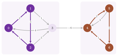
The program manual/examples/16-min-mean-cycle.cc (the test
manual_16_min_mean_cycle) solves the problem of Figure 16.1 with the three
classes, and checks that they agree on the mean \(4/3\) and that each cycle is
a closed walk with the cost and the length reported. It certifies the mean by
Theorem 16.1, since BellmanFord of chapter 10,
started with all the distances equal to 0, finds no negative cycle under the
costs \(|C|\,c(a)-c(C)\), and it checks that HowardMmc gives the two cycles
of the components, of means 2 and \(4/3\), and, with a limit of one iteration,
a cycle whose mean is not less than the optimal one.
In our view, the choice among the three is usually simple: HowardMmc is the
fastest in practice and the only one with the cycles of the components and the
limit on the iterations, while KarpMmc and HartmannOrlinMmc have the
polynomial bound \(O(nm)\) (Theorems 16.4 and 16.6), which may matter when the
running time must be bounded a priori.
16.6 Exercises
Exercise 16.1. Verify Theorem 16.1 on the
digraph of Figure 16.1 by computing with BellmanFord the potentials of
(16.2) for \(\mu=4/3\), scaled by 3 (the program
manual/examples/16-min-mean-cycle.cc checks only that no negative cycle
exists).
Exercise 16.2. Compute by hand the table
\(D_k(v)\) of (16.3) for the component \(\{4,5,6\}\) of Figure 16.1, with \(s=4\),
and evaluate (16.4); then compare cycleCost() and cycleSize() of KarpMmc
after findCycleMean() and after findCycle().
Exercise 16.3. Run the three classes on the four
cost functions of test/min_mean_cycle_test.cc, and check that they find the
cycles that the test expects (the test does it with checkMmcAlg()).
Exercise 16.4. For the cost function len1 of
test/min_mean_cycle_test.cc, find the least limit for which
HowardMmc::findCycleMean( limit ) returns OPTIMAL (the test checks that 2
iterations are not enough and 4 are).
Exercise 16.5. Use componentCycleNum() and
componentCycle() of HowardMmc to list, for a digraph with several strongly
connected components, the node-disjoint cycles of minimum mean of the
components, and keep those of negative mean, as unboundedCycles( k ) does
(the program of section 16.5 lists the two cycles of Figure 16.1).
Exercise 16.6. Check Lemma 16.1 (ii) with any of the three classes on the digraph of Figure 16.1, by adding the same constant to all the costs.
Exercise 16.7. Build a digraph on which
Algorithm 16.2 checks its certificate at round 4 while some node has no walk
of at most 4 arcs from \(s\), e.g., a cycle of 10 nodes through \(s\) with a loop
at \(s\) whose mean is not the least. Then compare the cycles found by
HartmannOrlinMmc with int costs and with SetLargeCost< double > (see
the remark after Theorem 16.5).