5. Graph adaptors¶
We are concerned in this chapter with the classes of lemon/adaptors.h, which
present a digraph or a graph to an algorithm as if it were another one,
without copying it. The other structure may have fewer nodes or arcs, reversed
arcs or no orientation at all, split nodes, or only the arcs of positive
residual capacity of a flow. An adaptor stores a pointer to the adapted
structure (and, possibly, to some maps), and it answers each query of the
graph concepts of chapter 4 by one or more queries on
that structure; hence, building it costs \(O(1)\) time and memory, while the
price is paid at each step of an iteration. Section 5.1 describes what the
adaptors have in common, sections 5.2 to 5.5 describe them one family at a
time (filters, orientation, residual digraph, node splitting), with the
results on the flows and the paths that the residual digraph and the split
digraph serve, and section 5.6 collects the exercises. Throughout the chapter,
\(n_0\) and \(m_0\) are the numbers of nodes and of arcs (or edges) of the adapted
structure.
5.1 Views of a graph¶
Each adaptor of the header conforms to concepts::Digraph or to
concepts::Graph (cf. chapter 3). Therefore, it
can be passed to the algorithms of the library and to the functions of
core.h, and it can be adapted again: the function checkCombiningAdaptors()
of test/adaptors_test.cc builds, e.g., an Undirector of a SplitNodes of
an Orienter of a GridGraph, and checks it against concepts::Graph. Three
properties are shared, in some form, by all the classes of the chapter, and we
state them once here.
Constness and modification. The first template parameter is the type of the
adapted structure, and it may be given as const (e.g.,
ReverseDigraph< const ListDigraph >). In that case the adaptor can be built
from a constant reference, and it offers no modifying function. Otherwise, the
adaptors that keep the item set of the adapted structure (ReverseDigraph,
SubDigraph, SubGraph, FilterNodes, FilterArcs, FilterEdges,
Undirector and Orienter) forward addNode(), addArc() (or addEdge()),
erase() and clear() to it, and one changes the adapted structure through
the adaptor. ResidualDigraph and SplitNodes, instead, take their digraph
as implicitly const, since an arc added to a residual digraph (or a node
added to a split digraph) has no meaning for the underlying one. Each adaptor
names the adapted structure by the type Digraph (or Graph, for the
adaptors of a graph), and the filtering adaptors also name their filters by
NodeFilterMap, ArcFilterMap and EdgeFilterMap. Each adaptor has a
creator function, i.e., reverseDigraph(), subDigraph(), subGraph(),
filterNodes(), filterArcs(), filterEdges(), undirector(),
orienter(), residualDigraph() and splitNodes(), which returns the
read-only version (the one on the const structure), with the filter maps
const or not as they are passed.
Items. The Node and Arc (and Edge) types of an adaptor are usually
convertible to and from those of the adapted structure, as the notes of the
header state class by class. For instance, a node of a SubDigraph is a node
of the digraph, and an edge of an Undirector is an arc of the digraph (the
exceptions are given where they occur). Hence, a map of the adapted structure
can be read with the items of the adaptor.
Maps and counting. For the adaptors that keep the item set, the NodeMap,
ArcMap and EdgeMap of the adaptor are maps of the adapted structure, and
they store a value for each of its items (the hidden ones included).
Undirector, ResidualDigraph and SplitNodes, whose arcs are not arcs of
the digraph, build their arc maps from two maps of the digraph. Counting by
countNodes(), countArcs() and countEdges() takes constant time on
ReverseDigraph, Undirector, Orienter and SplitNodes when the adapted
structure counts in constant time (SplitNodes counts by countNodes() and
countArcs() of the digraph, whatever the digraph does). The filtering
adaptors (and ResidualDigraph, which is one of them) count by iterating, in
linear time; in fact, their tags NodeNumTag and ArcNumTag are False.
In general, the cost of an iteration on an adaptor is that of the iteration on the adapted structure plus a constant amount of work per item visited (which is rather small). There is one exception, which may matter in practice: a filtering adaptor skips the hidden items one by one, since it has no list of the visible ones. The following lemma makes this precise.
Lemma 5.1. Let \(F\) be one of SubDigraph,
SubGraph, FilterNodes, FilterArcs, FilterEdges and ResidualDigraph,
and let \(v\) be a node of the adapted structure with \(h(v)\) outgoing arcs in
it. A complete iteration of OutArcIt over \(v\) on \(F\) visits each of the
\(h(v)\) arcs once and costs \(O(1+h(v))\) time, a single step of it may cost
\(\Theta(h(v))\), and a complete iteration of NodeIt or ArcIt costs
\(O(1+n_0)\) or \(O(1+n_0+m_0)\) time, provided that a read of a filter, a call of
firstOut(), nextOut(), first() and next() of the adapted structure
cost \(O(1)\). The same holds for InArcIt and, on the graphs, for IncEdgeIt
and EdgeIt.
Proof. The functions first(), firstOut(), next() and nextOut() of
the bases SubDigraphBase and SubGraphBase call the function of the same
name of the adapted structure, and then its next() (or nextOut()) while
the current item is hidden. Thus, the adapted iteration is advanced exactly
once per item, and each item is tested by at most three reads of the filters
(its own value and those of its two ends, or only its own for FilterArcs and
FilterEdges, whose template flag ch is false). A single step from a
visible arc to the next visible one passes over all the hidden arcs in
between, which may be all the others. For ResidualDigraph the adapted
structure is an Undirector, whose outgoing iteration over \(v\) visits the
arcs entering and leaving \(v\) in the digraph once each (section 5.3), and the
filter is read in \(O(1)\) (section 5.4). \(\square\)
Hence, an algorithm run on a filter that hides most of the items may be
(somewhat, or much) slower than the same algorithm run on a copy made with
digraphCopy() (cf. chapter 4). Of course, the copy
costs time and memory, and it does not follow the later changes of the filter.
We remark that FilterNodes, FilterArcs, FilterEdges and
ResidualDigraph hold, as members, objects to which their base class points
(the constant filter that replaces the one they lack and, for the residual
digraph, the inner Undirector and the filters of the residual capacities).
Their copy constructor and their assignment, therefore, point the copy to its
own members, so that a copy (e.g., the one returned by filterNodes() or
residualDigraph()) is independent of the object it was copied from and may
outlive it.
abLEMON
In LEMON 1.3.1, the implicit copy of these four adaptors copied the
pointers, which still referred to the members of the original, so that a
copy that outlived it (e.g., the value of residualDigraph() when the
compiler does not elide the copy) read freed memory;
checkAdaptorCopies() in test/adaptors_test.cc copies and assigns
each of them and uses the copy of a ResidualDigraph after the original
has been destroyed and overwritten.
The classes of the header are built on base classes that a user does not
instantiate, i.e., DigraphAdaptorBase and GraphAdaptorBase (which forward
each query to the adapted structure), ReverseDigraphBase, SubDigraphBase,
SubGraphBase, UndirectorBase, OrienterBase and SplitNodesBase (which
change the queries), completed by the extenders of lemon/bits/ (cf.
appendix A). The maps of Undirector and
SplitNodes are built on their private classes ArcMapBase and
NodeMapBase, and the arc filters of ResidualDigraph are the functors
ResForwardFilter and ResBackwardFilter of the namespace _adaptor_bits.
All the adaptors but ResidualDigraph and SplitNodes also have a protected
default constructor, which leaves the adaptor unbound, so that a derived class
may bind it later by the protected initialize() of its base (passing, for
FilterNodes, FilterArcs and FilterEdges, the member const_true_map as
the filter that the adaptor lacks).
abLEMON
In LEMON 1.3.1, the protected default constructor of FilterEdges called
a function setNodeFilterMap() that does not exist, so that a derived
class that used it did not compile; the class LateFilterEdges of
test/adaptors_test.cc uses it.
5.2 Reversing and filtering¶
ReverseDigraph< DGR > presents the digraph DGR with all its arcs reversed.
Its source() and target() are exchanged, the outgoing arcs of a node are
its incoming arcs in the digraph (and vice versa), findArc( u , v ) looks
for an arc from v to u in the digraph, and addArc( u , v ) adds the arc
\((v,u)\) to it. Its constructor takes the digraph
(explicit ReverseDigraph( DGR & digraph )), and the adaptor counts in the
time of the digraph. One typically uses it to run a search backwards, e.g., to
find the nodes from which a target is reachable, or to compute the distances
to a node by Dijkstra with the same length map.
The filtering adaptors hide some of the items by means of bool maps, called
filters: an item is visible if and only if its filter value is true.
SubDigraph< DGR , NF , AF > filters both the nodes and the arcs of a
digraph, with a node map NF and an arc map AF, whose defaults are
DGR::NodeMap< bool > and DGR::ArcMap< bool >. An arc is visible when it is
enabled and both its ends are enabled. SubGraph< GR , NF , EF > does the
same for a graph, with an edge filter EF (by default GR::EdgeMap< bool >),
and an edge is visible when it and both its ends are enabled. Three
specialized filters keep a constant map, i.e., a ConstMap with the inlined
value true (cf. §6.3), in place of the filter they
lack. FilterNodes< GR , NF > works on a digraph or on a graph (it chooses
the concept from the UndirectedTag of GR), and it hides the nodes together
with the arcs or edges incident to them. FilterArcs< DGR , AF > hides arcs
of a digraph, and FilterEdges< GR , EF > hides edges of a graph (and both
their arcs); neither of the two hides a node.
Their constructors take the structure and references to the filters, which the
adaptor keeps by pointer, e.g.,
SubDigraph( DGR & digraph , NF & node_filter , AF & arc_filter ) and
FilterArcs( DGR & digraph , AF & arc_filter ). Thus, the filters must
outlive the adaptor, and a value written directly into a filter is seen at
once through the adaptor. The same can be done through the adaptor itself:
status( item , v ) sets the filter value of the item to v and
status( item ) reads it, while enable( item ) and disable( item ) are
status( item , true ) and status( item , false ). Each of them costs one
access to the filter map (a FilterNodes has them for the nodes only, a
FilterArcs for the arcs, a FilterEdges for the edges). Building the
filters (e.g., DGR::ArcMap< bool > f( g , true ), which shows the whole
digraph) is left to the caller, since only the caller knows which items are to
be seen.
A SubDigraph with an all-true node filter and a FilterArcs show the same
digraph; the difference is one of efficiency. The former checks the filter
values of the two ends of each arc it visits (the template flag ch = true of
SubDigraphBase), while the latter, whose node filter is the constant true,
checks only the arc filter. The search of an arc between two nodes behaves as
follows.
Lemma 5.2. On a filtering adaptor,
findArc( u , v , prev ) (and, on the graphs, findEdge( u , v , prev ))
returns INVALID at once if u or v is hidden, and otherwise the first
visible arc from u to v that the adapted structure returns after prev,
or INVALID if there is none. It calls findArc() (or findEdge()) of the
adapted structure \(k+1\) times, where \(k\) is the number of hidden arcs that it
skips.
Proof. The function reads the node filter at u and v; then it calls
findArc( u , v , prev ) of the adapted structure and, while the arc returned
is hidden, calls it again from that arc. Each call either returns INVALID,
which ends the loop, or returns the next arc from u to v, which is either
the result or one of the \(k\) hidden arcs skipped. \(\square\)
5.3 Changing the orientation¶
Undirector< DGR > presents a digraph as an undirected graph. Each arc of the
digraph is an edge of the adaptor, with u( e ) its source and v( e ) its
target, and, as for the other graphs of the library, each edge also gives two
arcs: the forward one (direction( a ) == true), oriented as the arc of the
digraph, and the backward one. The Edge type of the adaptor is the Arc
type of the digraph, while its Arc is a pair (arc of the digraph,
direction), which converts to the arc of the digraph. The constructor takes
the digraph, addEdge( u , v ) adds the arc \((u,v)\) to it, and the ArcMap
of an Undirector keeps two arc maps of the digraph, one per direction. The
outgoing arcs of a node \(v\) are the backward arcs of the arcs that enter \(v\)
in the digraph, followed by the forward arcs of those that leave it; thus, an
outgoing iteration over \(v\) costs the in-degree plus the out-degree of \(v\) in
the digraph. Also, edgeNum() is arcNum() of the digraph and arcNum() is
twice as much, both in the time of the digraph, and findArc( s , t ) returns
first the forward arcs of the arcs from \(s\) to \(t\) and then the backward arcs
of those from \(t\) to \(s\). The identifiers obey the following rule.
Lemma 5.3. Let \(i\) be the identifier of an arc
of the digraph. In an Undirector, the edge of that arc has identifier \(i\),
its forward arc \(2i+1\) and its backward arc \(2i\); these are distinct for
distinct arcs of the adaptor, arcFromId() inverts id(), and they do not
exceed maxArcId(), which is \(2\,\)maxArcId()\(\,+1\) of the digraph.
Proof. The code computes id( a ) as \((i \ll 1) \mid d\), with \(d\) the
direction bit, and arcFromId( x ) as the arc of identifier \(x \gg 1\) with
the direction \(x \mathbin{\&} 1\); the two maps are inverse to each other, and
\(2i+d\le 2\max_i i+1\). \(\square\)
When an algorithm on the undirected graph needs an arc map and the data are on
the digraph, the nested class Undirector< DGR >::CombinedArcMap< FW , BK >
reads the forward arcs from the arc map FW and the backward ones from BK,
and its set() writes to the one of the two that the direction selects. It is
created by the static function combinedArcMap( forward , backward ), its
value type is that of FW, and it is a reference map when FW is one. For
instance, Undirector< const G >::combinedArcMap( cost , cost ) gives an
undirected length (or capacity) taken from one arc map of the digraph.
Orienter< GR , DM > goes the other way, and it presents a graph as a digraph
in which each edge is an arc. The arc goes from u( e ) to v( e ) when the
direction map DM (a bool edge map, by default GR::EdgeMap< bool >, named
by the type DirectionMap) is true on the edge, and from v( e ) to
u( e ) otherwise. Its constructor takes the graph and the direction map,
which is kept by pointer, and reverseArc( a ) negates the direction of an
arc by one write to the map. Furthermore, addArc( u , v ) adds an edge to
the graph and sets its direction, so that the new arc goes from u to v.
Since the arcs of the adaptor are the edges of the graph, arcNum() is
edgeNum() of the graph, and the identifier of an arc is that of its edge.
Lemma 5.4. On an Orienter, a complete
iteration of OutArcIt (or InArcIt) over a node \(v\) costs \(O(1+\deg(v))\),
where \(\deg(v)\) is the number of edges incident to \(v\) in the graph, and
findArc( u , v ) calls findEdge( u , v ) of the graph once for each edge
between \(u\) and \(v\) that it skips, plus one.
Proof. firstOut() and nextOut() iterate on the incident edges of \(v\) by
firstInc() and nextInc() of the graph and skip each edge whose direction
does not make \(v\) its source, i.e., they pass once over each incident edge.
Then findArc() calls findEdge() of the graph and repeats while the source
of the edge found is not u. \(\square\)
The function checkCombiningAdaptors() of test/adaptors_test.cc orients a
grid by an Orienter, splits its nodes and views the result through an
Undirector. The program manual/examples/05-filter-undirector.cc (the test
manual_05_filter_undirector) keeps by a FilterArcs the arcs of a digraph
whose cost is at most a threshold, and it counts the connected components of
the result through an Undirector before and after enabling one more arc. It
also finds by Bfs on a ReverseDigraph the nodes from which a node is
reached.
5.4 The residual digraph¶
Let \(G=(V,A)\) be a digraph, \(u: A\to\mathbb{R}_+\) a capacity, and \(s\ne t\) two nodes. A flow from \(s\) to \(t\) is a vector \(x\) with \(0\le x_a\le u_a\) for each arc \(a\) and with
and its value \(v(x)\) is the left-hand side of (5.1) at \(i=s\), i.e., the net flow out of \(s\). The residual digraph of \(x\) (cf. Ahuja, Magnanti and Orlin 1993, §2.4) has node set \(V\) and arc set \(A_f\cup A_b\), where
Each forward arc \((i,j)\in A_f\) has residual capacity \(r_{ij}=u_{ij}-x_{ij}\), and each backward arc \((j,i)\in A_b\) has residual capacity \(r_{ji}=x_{ij}\). The union is taken with multiplicity; thus, an arc of \(G\) may give two arcs of the residual digraph, and parallel arcs may appear (Figure 5.1). A directed path from \(s\) to \(t\) in the residual digraph is called an augmenting path, and its bottleneck is the least residual capacity of its arcs. For a set \(S\) of nodes with \(s\in S\) and \(t\notin S\) (a cut), its capacity is \(u(S)=\sum_{(i,j)\in A:\,i\in S,\,j\notin S}u_{ij}\).
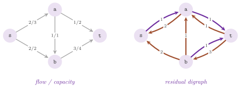
ResidualDigraph< DGR , CM , FM , TL > implements (5.2) as an adaptor. DGR
is the digraph (implicitly const), CM the capacity map (by default
DGR::ArcMap< int >, implicitly const), FM the flow map (by default
CM), which the adaptor may write, and TL the tolerance (by default
Tolerance< CM::Value >, cf. chapter 3). The class
names them by the types Digraph, CapacityMap, FlowMap and Tolerance,
and the value type of the capacities by Value. The tolerance decides which
arcs exist. A forward arc is there when
tolerance.positive( cap[a] - flow[a] ) holds, and a backward arc when
tolerance.positive( flow[a] ) holds; on floating-point data, an arc whose
residual capacity is below the epsilon of the tolerance is therefore hidden.
The class is a SubDigraph of an Undirector< const DGR > of the digraph,
with the constant true as node filter and, as arc filter, a CombinedArcMap
of these two tests (the note of the header calls it a combination of
Undirector and FilterArcs, which describes the effect). Hence, an arc of
the adaptor is an arc of the Undirector (convertible to the arc of the
digraph it comes from), the adaptor counts in linear time, and its iterations
skip the arcs of zero residual capacity one by one (Lemma 5.1). The
constructor ResidualDigraph( digraph , capacity , flow , tolerance ) takes
the digraph and the capacity map by constant reference, the flow map by
reference and the tolerance by constant reference, by default Tolerance(),
and the members that are specific to the residual digraph are the following.
residualCapacity( a )returns \(u_a-x_a\) for a forward arc and \(x_a\) for a backward one, computed without the tolerance.augment( a , v )addsvto the flow of the original arc ifais forward, and it subtractsvifais backward. It writes the flow map byset(), and it does not check that the result stays within the bounds.forward( a )andbackward( a )(static), on an arc of the adaptor, give its direction. On an arc of the digraph, they return the forward or the backward residual arc that corresponds to it, whether or not that arc is currently visible.ResidualCapacityis a read-only arc map of the adaptor whose value at an arc isresidualCapacity( a ). It is created byresidualCapacity(), and its value type is that of the capacity map.
The function residualDigraph( digraph , capacity , flow ) returns the
adaptor with the default tolerance.
The augmenting path method of Ford and Fulkerson 1956 needs only the residual digraph, and Algorithm 5.1 writes it with the classes of the library; the choice of a shortest path, i.e., of a path found by a breadth-first search, is the rule of Edmonds and Karp 1972.
Algorithm 5.1 (Augmenting paths on the residual digraph).
input:  digraph G, capacity u, flow x from s to t (e.g., x = 0)
R := ResidualDigraph(G, u, x)
loop
  run Bfs on R from s, stopped when t is reached     (bfs.run(s, t))
  if t is not reached then stop
  P := the path from s to t of the search tree        (bfs.path(t))
  delta := min { residualCapacity(a) : a in P }
  for each arc a of P: augment(a, delta)
end loop
output: x, a maximum flow; S, the nodes reached by the last search,
        the source side of a minimum cut
The correctness of the algorithm rests on three facts, which we prove in turn: an augmentation keeps \(x\) a flow and increases its value, a flow is maximum exactly when no augmenting path exists, and the search by shortest paths bounds the number of augmentations.
Lemma 5.5. Let \(x\) be a flow from \(s\) to \(t\), \(P\) an augmenting path of its residual digraph with no repeated node, and \(0<\delta\le\min_{a\in P}r_a\). Augmenting \(x\) by \(\delta\) along \(P\) (adding \(\delta\) to the flow of the original arc of each forward arc of \(P\), and subtracting it from that of each backward arc) gives a flow \(x'\) from \(s\) to \(t\) with \(v(x')=v(x)+\delta\).
Proof. On the original arc of a forward arc the flow grows by \(\delta\le u_a-x_a\), and on that of a backward arc it drops by \(\delta\le x_a\); hence, \(0\le x'\le u\). An inner node \(i\) of \(P\) is entered by one arc of \(P\) and left by one. Each of the two changes the net flow out of \(i\) by \(\delta\) in opposite directions (a forward arc entering \(i\) adds \(\delta\) to the flow into \(i\), a backward arc entering \(i\) removes \(\delta\) from the flow out of \(i\), and symmetrically for the arc leaving \(i\)); thus, (5.1) still holds. At \(s\), the first arc of \(P\) either adds \(\delta\) to an arc leaving \(s\) or removes it from an arc entering \(s\), and no arc of \(P\) enters \(s\); hence, \(v(x')=v(x)+\delta\). \(\square\)
Theorem 5.1. (Maximum flow and minimum cut.) For every flow \(x\) from \(s\) to \(t\) and every cut \(S\), \(v(x)\le u(S)\). A flow \(x\) is maximum if and only if its residual digraph has no path from \(s\) to \(t\); in that case, the set \(S\) of the nodes reachable from \(s\) in the residual digraph is a cut with \(u(S)=v(x)\), i.e., a minimum cut.
Proof. Summing (5.1) over the nodes of \(S\setminus\{s\}\) and adding the definition of \(v(x)\) gives \(v(x)=\sum_{i\in S,\,j\notin S}x_{ij}-\sum_{j\notin S,\,i\in S}x_{ji}\), where the sums run over the arcs of \(G\) that leave and that enter \(S\), since the arcs with both ends in \(S\) cancel. Then \(0\le x\le u\) gives \(v(x)\le u(S)\). If the residual digraph has an augmenting path, it also has one with no repeated node, and Lemma 5.5 gives a flow of larger value; hence, \(x\) is not maximum. Conversely, let no path exist and let \(S\) be the set of the nodes reachable from \(s\), so that \(s\in S\) and \(t\notin S\). No residual arc leaves \(S\); by (5.2), each arc of \(G\) from \(S\) to \(V\setminus S\) has \(x_{ij}=u_{ij}\), and each arc from \(V\setminus S\) to \(S\) has \(x_{ji}=0\). The identity above then gives \(v(x)=u(S)\), and the first part shows that no flow exceeds \(u(S)\). \(\square\)
Theorem 5.2. If the capacities and the initial
flow are integers, Algorithm 5.1 (with the default tolerance, under which
positive( y ) is \(y>0\)) terminates; its final flow is maximum and integral,
and the set \(S\) is a minimum cut. Hence, on integral capacities a maximum flow
exists whose values are integers.
Proof. By induction, all the flows and residual capacities stay integral,
since \(\delta\) is a minimum of integers; each augmentation increases the value
by \(\delta\ge1\) (Lemma 5.5, where the path of the search tree has no repeated
node), and the value is bounded by \(u(\{s\})\) (Theorem 5.1). Therefore, the
algorithm stops, which happens when the complete search from \(s\) does not
reach \(t\) (run( s , t ) stops early only when it reaches \(t\)); the reached
nodes are then all the nodes reachable from \(s\), and Theorem 5.1 applies.
\(\square\)
On floating-point data the arcs of residual capacity below the epsilon of the tolerance are hidden; hence, at the end no augmenting path of bottleneck larger than that epsilon remains, and the flow is maximum only up to a quantity of that order per arc of the final cut. The number of augmentations is bounded independently of the capacities when the paths are shortest.
Theorem 5.3. (Edmonds and Karp.) Let \(n=|V|\) and \(m=|A|\). Algorithm 5.1 makes at most \(nm\) augmentations, whatever the capacities, and it runs in \(O(nm(n+m))\) time.
Proof. Let \(d_x(i)\) be the number of arcs of a shortest path from \(s\) to \(i\)
in the residual digraph \(R(x)\) (\(+\infty\) if none). Let \(x'\) be obtained from
\(x\) by an augmentation along a shortest path \(P\). Every arc of \(R(x')\) that is
not in \(R(x)\) is the reverse of an arc \((i,j)\) of \(P\), for which
\(d_x(j)=d_x(i)+1\). Hence, every arc \((a,b)\) of \(R(x')\) satisfies
\(d_x(b)\le d_x(a)+1\), and, by induction along a shortest path of \(R(x')\),
\(d_x(i)\le d_{x'}(i)\) for every node \(i\): the distances never decrease. An arc
of \(P\) whose residual capacity equals \(\delta\) (one exists) is called
critical, and it leaves the residual digraph. Let \((i,j)\) be critical at \(x\),
so that \(d_x(j)=d_x(i)+1\). Before \((i,j)\) is critical again it must reappear,
which requires an augmentation, at some flow \(z\), along a shortest path that
contains \((j,i)\); then \(d_z(i)=d_z(j)+1\ge d_x(j)+1=d_x(i)+2\). Since a node on
an augmenting path other than \(t\) has distance at most \(n-2\), the residual arc
\((i,j)\) is critical at most \(n/2\) times. The residual arcs are the forward and
the backward arc of each arc of \(G\), i.e., \(2m\) of them, and each augmentation
has a critical arc; hence, there are at most \(nm\) augmentations. Each
iteration costs one breadth-first search on the adaptor, i.e., \(O(n+m)\) time
by Lemma 5.1 (an outgoing iteration over \(i\) on the Undirector visits the
arcs entering and leaving \(i\) in \(G\)), plus \(O(n)\) for the path and the
augmentations. \(\square\)
The library has faster maximum flow algorithms, Preflow and EdmondsKarp
(cf. chapter 12). In our view, the adaptor is meant,
rather, for the algorithms that search the residual digraph of a flow already
found, e.g., for a minimum cut, for the cycles of a circulation, or for a
shortest path of reduced costs. The program
manual/examples/05-residual-augment.cc (the test
manual_05_residual_augment) runs Algorithm 5.1 on a digraph of five nodes,
and it checks the value of the flow and the capacity of the cut of Theorem 5.1
against Preflow. The function checkResidualDigraph() of
test/adaptors_test.cc checks the members of the adaptor and augments along
shortest paths on another digraph.
5.5 Splitting the nodes¶
Several network problems (often, but not always, routing problems) put a bound or a cost on the nodes (the number of paths through a node, the capacity of a switch, the cost of a visit), while the algorithms of the library take them on the arcs. The standard transformation (cf. Ahuja, Magnanti and Orlin 1993, §2.4) replaces each node \(w\) of \(G\) by two nodes \(w_{in}\) and \(w_{out}\), joined by the bind arc \((w_{in},w_{out})\), which carries the data of the node; each arc \((v,w)\) of \(G\) becomes the arc \((v_{out},w_{in})\), called an original arc (Figure 5.2). We denote by \(G'\) the digraph so obtained, which has \(2n\) nodes and \(m+n\) arcs.
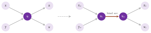
Lemma 5.6. Let \(s\ne t\). The map that sends a path \((s=w_0,a_1,w_1,\dots,a_k,w_k=t)\) of \(G\) with no repeated node to the path of \(G'\) that starts at \(s_{out}\), takes the original arc of each \(a_h\) and, between two of them, the bind arc of \(w_h\) (\(0<h<k\)), is a bijection between the \(s\)-\(t\) paths of \(G\) with no repeated node and the \(s_{out}\)-\(t_{in}\) paths of \(G'\) with no repeated node. These never use the bind arcs of \(s\) and \(t\), and they use the bind arc of \(w\) exactly when the path of \(G\) passes through \(w\) as an inner node.
Proof. In \(G'\) the only arc leaving an in-node is its bind arc, and the only arc entering an out-node is its bind arc. Hence, a path of \(G'\) from \(s_{out}\) alternates an original arc, which ends at an in-node, and the bind arc of that node, until it ends at \(t_{in}\); the bind arc of \(s\) would enter \(s_{out}\) again, and that of \(t\) would leave \(t_{in}\), so a path with no repeated node uses neither. Reading the original arcs in order gives a path of \(G\) from \(s\) to \(t\), which has no repeated node since each node \(w\) of it gives the distinct nodes \(w_{in}\) and \(w_{out}\); this is the inverse of the map of the statement. \(\square\)
SplitNodes< DGR > implements the transformation on the digraph DGR, which
is implicitly const. A node of the adaptor is a node of the digraph with a
flag (in or out), and it converts to the node of the digraph. An arc, instead,
is either an arc or a node of the digraph (a BiVariant); it has conversions
to both types, of which only the one that matches its kind is meaningful (that
to the arc for an original arc, that to the node for a bind arc). The
identifiers are \(2i\) for the in-node and \(2i+1\) for the out-node, and \(2i\) for
an original arc and \(2i+1\) for the bind arc of a node, where \(i\) is the
identifier in the digraph, so that maxArcId() is the larger of
\(2\,\)maxArcId() and \(2\,\)maxNodeId()\(\,+1\) of the digraph. nodeNum() and
arcNum() are computed by countNodes() and countArcs() of the digraph,
i.e., in the time of the digraph. Also, findArc( u , v ) returns the bind
arc when u is the in-node and v the out-node of the same node, the
original arcs found by findArc() of the digraph when u is an out-node and
v an in-node, and INVALID otherwise. Besides the types Digraph,
DigraphNode and DigraphArc, the static members translate between the two
structures, as follows.
inNode( n )andoutNode( n ), on a node of the adaptor, return which of the two it is; on a node of the digraph, they return its in-node or its out-node.origArc( a )andbindArc( a )return whether an arc of the adaptor is an original arc or a bind arc.arc( n )returns the bind arc of a node of the digraph, andarc( a )the arc of the adaptor that corresponds to an arc of the digraph.
abLEMON
In LEMON 1.3.1, maxArcId() of SplitNodes was the larger of
\(2\,\)maxNodeId() and \(2\,\)maxArcId()\(\,+1\) of the digraph, below
the identifier of the last bind arc when the digraph has more nodes than
arcs; checkSplitNodes() in test/adaptors_test.cc checks a digraph of
two nodes and no arc.
One gives the data by two combining maps, nested in the class.
CombinedNodeMap< In , Out >, created by
combinedNodeMap( in_map , out_map ), reads the in-nodes from the node map
In and the out-nodes from Out. CombinedArcMap< AM , NM >, created by
combinedArcMap( arc_map , node_map ), reads the original arcs from the arc
map AM and the bind arcs from the node map NM. Their value types are those
of In and AM, respectively, and their set() writes to the map that the
kind of the item selects. In this way, one may turn a node capacity into the
capacity of a bind arc, and the following form of the theorem of Menger
1927 (cf. Ahuja, Magnanti and
Orlin 1993, §6.6) computes the
largest number of paths with no inner node in common as a maximum flow.
Theorem 5.4. Let \(s\ne t\), and give \(G'\) integral capacities: 1 on the bind arc of each node other than \(s\) and \(t\), 1 on the original arcs of the arcs from \(s\) to \(t\), at least 1 on the other original arcs, and any value on the bind arcs of \(s\) and \(t\). The value of a maximum flow from \(s_{out}\) to \(t_{in}\) in \(G'\) equals the largest number of distinct \(s\)-\(t\) paths of \(G\) with no repeated node and no inner node in common.
Proof. Let \(P_1,\dots,P_k\) be such paths. By Lemma 5.6 their images in \(G'\) are paths from \(s_{out}\) to \(t_{in}\); two of them share no bind arc, since they have no inner node in common, and no original arc, since an arc of \(G\) with an inner end belongs to one path only and an arc from \(s\) to \(t\) is a path by itself. Sending one unit along each image gives a flow of value \(k\) within the capacities. Conversely, by Theorem 5.2 there is a maximum flow \(y\) of integral values, say of value \(k\). An integral flow of value \(k\) is the sum of \(k\) unit flows along paths from \(s_{out}\) to \(t_{in}\) with no repeated node and of a circulation. To see this, start from \(s_{out}\) and follow arcs of positive flow, which exist by (5.1) at each node other than \(t_{in}\), until \(t_{in}\) is reached or a node repeats; in the first case subtract one unit along the path, in the second along the cycle, and repeat (each step lowers the sum of the flows, cf. the flow decomposition of Ahuja, Magnanti and Orlin 1993, §3.5). The \(k\) unit paths map to \(s\)-\(t\) paths of \(G\) by Lemma 5.6. Two of them that shared an inner node \(w\) would carry two units on the bind arc of \(w\), whose capacity is 1, and two of them that were the same arc from \(s\) to \(t\) would carry two units on it. Hence, they are \(k\) distinct paths with no inner node in common. \(\square\)
The program manual/examples/05-split-nodes.cc (the test
manual_05_split_nodes) computes in this way, by Preflow on a SplitNodes,
the largest number of paths with no inner node in common in a digraph of six
nodes, and it checks that the split digraph has 12 nodes and 14 arcs.
5.6 Exercises¶
Exercise 5.1. Write the type of the adaptor that
presents the subgraph of a ListDigraph induced by a set of nodes, with the
arcs reversed, to an algorithm that takes a const digraph. Say which of its
operations cost more than the corresponding operation of the digraph (Lemmas
5.1 and 5.2). The functions checkReverseDigraph() and checkSubDigraph() of
test/adaptors_test.cc check the two adaptors separately.
Exercise 5.2. Modify
manual/examples/05-residual-augment.cc so that each augmentation uses a path
of largest bottleneck capacity (a "widest" path) instead of a shortest one,
and compare the number of augmentations on a digraph with "large" capacities.
The value must still agree with Preflow.
Exercise 5.3. Build a digraph with two parallel
arcs and an arc in each direction between two nodes, give it a flow that is
positive and below the capacity on each arc. Then check with countArcs()
that the residual digraph has \(|A_f|+|A_b|\) arcs (cf. (5.2)), and with
findArc() that it returns all of them between the two nodes (Lemma 5.2).
Exercise 5.4. Starting from
manual/examples/05-split-nodes.cc, use SplitNodes and a minimum cost flow
algorithm (cf. chapter 13) to find \(k\) paths from
\(s\) to \(t\) with no inner node in common and of least total length, and prove,
along the lines of Theorem 5.4, that the paths found have this property.
Exercise 5.5. Given an undirected graph and an
orientation of its edges in a bool edge map, use Orienter and an algorithm
for the strongly connected components (cf. chapter
18) to decide whether the orientation is strongly
connected. Then reverse one arc by reverseArc() and decide again, without
rebuilding anything; the function checkOrienter() of test/adaptors_test.cc
checks reverseArc().