13. Minimum cost flows¶
We are concerned in this chapter with the four minimum cost flow algorithms of
the library, NetworkSimplex (lemon/network_simplex.h), CostScaling
(lemon/cost_scaling.h), CapacityScaling (lemon/capacity_scaling.h) and
CycleCanceling (lemon/cycle_canceling.h), and with the concept
concepts::MinCostFlow of lemon/concepts/min_cost_flow.h that they meet. We
also describe two internal headers that a user meets through their effects,
i.e., the default tolerances of lemon/bits/mcf_tolerance.h, and the starting
flow and the bound on the infinite capacities of
lemon/bits/mcf_feasible_flow.h. Section 13.1 states the problem in the forms
that the library takes, together with its optimality conditions; section 13.2
describes the interface that the four classes share, and section 13.3 the way
in which they handle floating-point data. Sections 13.4 to 13.8 describe the
algorithms one by one, and section 13.9 gives some advice on the choice among
them. In chapter 14 we treat the certificates that
the four classes give when a problem has no optimal flow, and the classes that
enumerate several flows. As in chapter 12, the results
are stated in exact arithmetic, and section 13.3 describes what the tolerances
change in floating point.
13.1 The problem, its forms and its dual¶
Let \(G=(V,A)\) be a digraph with \(n\) nodes and \(m\) arcs, and let \(lower:
A\rightarrow\mathbf{R}\) and \(upper: A\rightarrow\mathbf{R}\cup\{+\infty\}\),
with \(lower\leq upper\), be bounds on the flow of the arcs. Let also \(cost:
A\rightarrow\mathbf{R}\) be the cost of a unit of flow on each arc, and \(sup:
V\rightarrow\mathbf{R}\) the signed supplies of the nodes (a supply if
positive, a demand if negative). Following Ahuja, Magnanti and Orlin
1993 and the page
doc/min_cost_flow.dox of the documentation, the library solves the problem
in the form with "greater or equal" supply constraints (GEQ):
Since the left-hand sides sum to zero, (13.1) can be feasible only if
\(\sum_{u\in V} sup(u)\leq 0\). Thus, the supplies must all leave their nodes,
while some demand may be left unmet. When the supplies sum to zero, the
constraints hold as equalities, and (13.1) is the usual equality form of the
problem; a user who wants that form must therefore make the supplies sum to
zero. In addition, NetworkSimplex takes the opposite form with "less or
equal" constraints (LEQ),
which needs \(\sum_{u\in V} sup(u)\geq 0\), and in which the demands must be met
while some supply may stay at its node. The other three classes take only the
GEQ form; one can bring the LEQ form to it by reversing the arcs and negating
the supplies, e.g., with ReverseDigraph (chapter 5)
and NegMap (chapter 6).
In the dual problem the variables are the potentials \(\pi: V\rightarrow\mathbf{R}\) of the nodes, and the reduced cost of an arc under them is
Hence, the potentials are the opposite of the prices of the textbook convention, in which \(cost^\pi(uv)=cost(uv)-\pi(u)+\pi(v)\); we keep the sign of the library throughout. We write \(N_f(u)=\sum_{uv\in A} f(uv)-\sum_{vu\in A} f(vu)\) for the net flow out of \(u\). The residual network of a feasible flow \(f\) has an arc \(uv\) of residual capacity \(upper(uv)-f(uv)\) and cost \(cost(uv)\) wherever \(f(uv)<upper(uv)\), and an arc \(vu\) of residual capacity \(f(uv)-lower(uv)\) and cost \(-cost(uv)\) wherever \(f(uv)>lower(uv)\). The optimality conditions rest on an identity, which one obtains by expanding (13.3) and collecting the terms of each node: for any flow \(g\) and any potentials \(\pi\),
Theorem 13.1. A feasible flow \(f\) of (13.1) is optimal if and only if there are potentials \(\pi\) such that, for each arc \(uv\) and each node \(u\),
For the LEQ form the same holds with \(\pi(u)\geq 0\) in place of \(\pi(u)\leq 0\). If the supplies sum to zero, the conditions on the signs of the potentials may be dropped.
Proof. Sufficiency. For a feasible flow \(g\), (13.4) gives \(\sum cost\cdot g = \sum cost^\pi g - \sum \pi(u) N_g(u)\). Each term of the first sum is at least \(cost^\pi(uv)\,lower(uv)\) if \(cost^\pi(uv)>0\) and at least \(cost^\pi(uv)\,upper(uv)\) if \(cost^\pi(uv)<0\), and each term \(-\pi(u)N_g(u)\) is at least \(-\pi(u)sup(u)\), since \(\pi(u)\leq 0\) and \(N_g(u)\geq sup(u)\). The conditions (13.5) state that \(f\) attains all these lower bounds, so that no feasible flow costs less than \(f\). Necessity. Add a node \(r\) of supply \(-\sum_{u\in V}sup(u)\geq 0\) and, for each node \(u\), an arc \(ru\) of cost 0 and infinite capacity. A flow \(f\) of (13.1) gives a flow of the equality form of this network, with \(N_f(u)-sup(u)\) on the arc \(ru\), and conversely; the two problems have the same optimal flows. If \(f\) is optimal, its residual network in the larger problem has no cycle of negative cost, since one unit (or the smallest residual capacity, if smaller) along such a cycle would decrease the cost. Hence, the cost \(d(u)\) of a shortest residual path to \(u\) from an extra node joined to all the nodes by arcs of cost 0 is finite and nonpositive. Also, \(d(v)\leq d(u)+c\) for each residual arc \(uv\) of cost \(c\), i.e., the reduced costs under \(d\) are nonnegative on the residual arcs. An arc with \(f<upper\) thus has \(cost^d\geq 0\), and one with \(f>lower\) has \(cost^d\leq 0\), which are the conditions of (13.5) on the arcs. The arc \(ru\) is always residual, so that \(d(u)\leq d(r)\), and if it carries flow, i.e., if \(N_f(u)\neq sup(u)\), its reverse is residual too, so that \(d(u)=d(r)\); hence, \(\pi=d-d(r)\) satisfies (13.5). For the LEQ form one adds arcs \(ur\) instead, and the signs change. When the supplies sum to zero, the last sum of (13.4) is the same for every feasible flow, and the argument holds for potentials of any sign. \(\square\)
This is the duality theorem of linear programming for (13.1); see Ahuja, Magnanti and Orlin 1993, chapter 9. Its proof also gives the following characterization, due to Klein 1967, which underlies the cycle canceling methods of section 13.8 and the final potentials of cost scaling.
Theorem 13.2. (Negative cycle optimality.) A feasible flow of the equality form is optimal if and only if its residual network has no directed cycle of negative cost. Then (13.5) holds for the potentials \(d\), where \(d(u)\leq 0\) is the cost of a shortest residual path to \(u\) from an extra node joined to all the others by arcs of cost zero.
Proof. A negative cycle allows a cheaper flow, as in the proof of Theorem 13.1. If there is none, the distances \(d\) are finite and give nonnegative reduced costs on the residual arcs, i.e., the conditions of (13.5) on the arcs, and \(d\leq 0\); by the sufficiency part of Theorem 13.1, in which the signs do not matter when the supplies sum to zero, \(f\) is optimal. \(\square\)
Three outcomes are possible, and run() returns them as the constants of the
nested enum ProblemType of each class. With OPTIMAL a flow and potentials
meeting (13.5) were found; with INFEASIBLE no flow satisfies the
constraints; and with UNBOUNDED the problem is feasible, while a directed
cycle of negative cost, whose arcs have infinite upper bounds, lets the cost
decrease without limit. An infinite upper bound is the constant INF of the
class, i.e., the infinity of Value if the type has one and its largest value
otherwise. The four algorithms only add and subtract residual capacities,
supplies and bounds (and the bound \(B\) of section 13.5, which is integer on
integer data); hence, on integer data they keep the flow integer, and the
optimal flow that they return is integer. In particular, an integer problem
that has an optimal flow has an integer one.
13.2 The common interface¶
All four classes take as template parameters the type GR of the digraph, the
number type V of the flows, of the bounds and of the supplies (by default
int), and the number type C of the costs and of the potentials (by default
V). They name them Value and Cost, and both must be signed, as the
constructors assert. CostScaling and CapacityScaling take a fourth
parameter, a traits class, which we describe with them. The constructor takes
the digraph, which must not change afterwards unless reset() is called; that
of NetworkSimplex takes a second argument, arc_mixing (section 13.4). The
parameters of the problem are then given by functions that copy the data at
once, so that the maps need not outlive the call; each returns the object.
lowerMap( map )sets the lower bounds, zero on the arcs if it is not called.upperMap( map )sets the upper bounds,INFon the arcs if it is not called.costMap( map )sets the costs, 1 on the arcs if it is not called.supplyMap( map )sets the supplies, zero if neither it norstSupply()is called, andstSupply( s , t , k )gives \(k\) to \(s\), \(-k\) to \(t\) and zero to the other nodes.supplyType( type ), inNetworkSimplexonly, sets the form,GEQ(the default) orLEQ, constants of the nested enumSupplyType.
Then run() solves the problem and returns its ProblemType, with arguments
that differ from class to class (Table 13.1). After a run, the queries are
totalCost(), i.e., the cost of the flow in \(O(m)\) time, flow( arc ) and
flowMap( map ), which give the flow, and potential( node ) and
potentialMap( map ), which give the potentials. With a template argument,
e.g., totalCost< double >(), the sum is made in another type, which helps
when it may overflow Cost. We describe the certificates infeasibleCut(),
infeasibleCuts( k ), disjointInfeasibleCuts(), unboundedCycle() and
unboundedCycles( k ), which are meaningful after a run that returned
INFEASIBLE or UNBOUNDED, in chapter 14, and
the tolerances in section 13.3.
One may call run() again: the parameters are kept, and only those that
changed have to be given anew. resetParams() sets the parameters back to
their defaults (and the supply type to GEQ), while reset() also rebuilds
the internal copy of the digraph, as is needed when the digraph itself was
modified after the construction or after the last reset(). In any case a
second run solves the problem from scratch, whatever changed. A typical use is
NetworkSimplex< ListDigraph > ns( g );
ns.upperMap( cap ).costMap( cost ).supplyMap( sup );
if( ns.run() == NetworkSimplex< ListDigraph >::OPTIMAL )
 c = ns.totalCost();
and the other three classes are called in the same way.
Table 13.1. The four classes: the arguments of
run() with their defaults, the worst case running time stated in each header
(\(U\) is the largest supply or capacity, \(K\) the largest absolute value of a
cost), the supply types, and the template parameters beyond GR, V and C.
| Class | run() |
Worst case | Forms | Traits |
|---|---|---|---|---|
NetworkSimplex |
pivot_rule = BLOCK_SEARCH |
not stated | GEQ, LEQ | none |
CostScaling |
method = PARTIAL_AUGMENT, factor = 16 |
\(O(n^2m\log(nK))\) | GEQ | LargeCost |
CapacityScaling |
factor = 4 |
\(O(m\log U\,(n+m)\log n)\) | GEQ | Heap |
CycleCanceling |
method = CANCEL_AND_TIGHTEN |
\(O(n^2m^2\log n)\) | GEQ | none |
All four meet the concept concepts::MinCostFlow< GR , V , C > of
lemon/concepts/min_cost_flow.h. It requires the constructor from the
digraph, reset(), resetParams(), the five setters of the parameters
(without supplyType()), run() with its defaults, the queries above, the
tolerance functions and types of section 13.3, and the single certificates
infeasibleCut() and unboundedCycle(). A function template written against
these members accepts any of the four, as does the function optimal() of the
program manual/examples/13-min-cost-flow.cc (the test
manual_13_min_cost_flow). This program solves a transshipment problem of
seven nodes with the four classes, and it checks that their costs agree (36)
and that the flow and the potentials of each meet (13.5). Then it runs
NetworkSimplex again after a change of one cost (66); finally it gives two
more units of supply to one node, which makes the problem infeasible in the
GEQ form and leaves an optimal flow, with nonnegative potentials, in the LEQ
form.
abLEMON
The four classes answer OPTIMAL, with the empty flow, on a digraph
without nodes, which LEMON 1.3.1 reported as infeasible. They answer
UNBOUNDED on the same problems, i.e., the feasible ones with a cycle of
negative cost made of arcs of infinite upper bound: in LEMON 1.3.1
CostScaling and CycleCanceling gave that answer on any arc of negative
cost and infinite upper bound, CapacityScaling gave a wrong answer on
feasible problems that its finite replacement of the infinite bounds made
infeasible, and NetworkSimplex did not check feasibility first. The
function runWarm(), which versions 1.4.0 to 1.5.0 added to re-optimize
from the last basis, flow or potentials, was removed in 1.6.0: a
re-optimization belongs to whoever knows what has changed, and a second
run() solves the changed problem.
13.3 Tolerances and floating-point data¶
With integer types the data must be integer, and the comparisons are exact.
With floating-point types the data need not be integer; however, a comparison
of a residual capacity or of a reduced cost with an exact zero would make the
algorithms pivot or push round-off for ever, or find a feasible problem
infeasible. Instead, the four classes compare against two tolerances, one on
the flows and one on the reduced costs, defined once in
lemon/bits/mcf_tolerance.h. Unless the caller sets them, they are zero for
an exact type and otherwise
where \(\varepsilon\) is the machine epsilon of the type (about \(2.2\cdot
10^{-16}\) for double), and the maxima run over the nodes and the arcs, with
the infinite upper bounds (and the values equal to the largest of the type)
left out. In other words, the tolerances are \(10^6\) units in the last place of
the largest datum, or of 1 when the data are smaller. An excess, a deficit or
a residual capacity within \(\epsilon_f\) is taken as zero, and a reduced cost
above \(-\epsilon_c\) as nonnegative. Also, a sum of the supplies within
\(\epsilon_f\) of zero is taken as zero, since supplies such as \(0.1\), \(0.2\) and
\(-0.3\), which sum to zero in decimal, in binary sum to a few units in the last
place of either sign.
A call of tolerances( flow , cost ) sets the two tolerances, and a negative
value, the default, leaves them to (13.6). In turn, flowTolerance() and
costTolerance() return the tolerances in use, as a Tolerance< Value > and
a Tolerance< Cost > (types named FlowTolerance and CostTolerance in each
class) whose epsilon is zero for an exact type. We remark that
NetworkSimplex computes them from its data at any time, while the other
three return those that the last run() used, and zero before the first one.
A tolerance of zero reproduces the behavior of LEMON 1.3.1, in which rounding
errors may keep the algorithm going for ever; hence, one should set it only on
data known to be exact in binary. The theorems of this chapter hold in
floating point only up to these tolerances. The program
manual/examples/13-floating-point.cc (the test manual_13_floating_point)
solves with the four classes a problem whose supplies are \(0.1\), \(0.2\) and
\(-0.3\) and whose capacities and costs are fractional. It checks the optimal
cost, \(0.14\), and the tolerances (13.6), which here are \(10^6\varepsilon\) on
the flows (the data being below 1) and \(1.1\cdot 10^6\varepsilon\) on the
costs; then it sets other tolerances, which flowTolerance() returns.
abLEMON
The four algorithms solve problems with floating-point costs, capacities
and supplies. In LEMON 1.3.1 NetworkSimplex compared reduced costs and
residual flows with an exact zero, and typically pivoted for ever or
reported infeasibility on such data, while the other three required
integer data and answered INFEASIBLE on supplies that sum to zero in
decimal but not in binary. The default tolerances have one definition for
the four (version 1.9.0), those of NetworkSimplex on the flows counting
the finite bounds too, and tolerances(), flowTolerance() and
costTolerance() are new.
13.4 The network simplex method¶
13.4.1 Bases, pivots and potentials¶
NetworkSimplex implements the primal network simplex method (Dantzig
1963; Ahuja, Magnanti and Orlin
1993, chapter 11; Kelly and O'Neill
1991), i.e., the simplex
method of linear programming specialized to (13.1), in which a basis is a
spanning tree. After moving the lower bounds into the supplies, the class adds
an artificial root node \(r\) and, for each node, an artificial arc between it
and the root, oriented by the sign of its supply; the initial basis is the
tree of these arcs, which carry the supplies. When the supplies do not sum to
zero, a second set of artificial arcs, of cost zero and infinite capacity,
lets the nodes keep the unmet demand (GEQ, arcs \(ru\)) or the unused supply
(LEQ, arcs \(ur\)). The artificial arcs of the tree whose flow would leave a
constraint violated (under GEQ those into the root, under LEQ and in the
balanced case those out of it) have a large cost \(M\), while the others cost
zero. For an exact Cost, \(M\) is half of the largest value of the type plus
one; otherwise \(M=(1+K)\,n\), where \(K=\max_{uv}|cost(uv)|\). Thus, the method
is the "big-M" variant of the simplex method on an auxiliary problem of \(n+1\)
nodes in the equality form, which is always feasible, and the problem is
infeasible exactly when some flow is left at the end on the artificial arcs
that may carry none (Theorem 13.3).
Each nonbasic arc is at its lower or at its upper bound, and the potentials are those that give a zero reduced cost to the arcs of the tree; they are unique up to a constant, since the tree spans the nodes. A nonbasic arc \(e\) is eligible if its reduced cost (13.3) is negative at its lower bound, or positive at its upper bound. Sending one unit around the cycle that \(e\) closes with the tree, in the direction allowed by its bound, changes the cost by its reduced cost (taken with the opposite sign at the upper bound), since the tree arcs have a zero reduced cost; hence, an eligible arc is one along whose cycle the cost decreases. A pivot chooses an eligible arc by the pivot rule, and finds its cycle through the join node, i.e., the first common ancestor of its ends in the tree. Then it sends around the cycle the largest amount \(\delta\) that the bounds allow, and it replaces by the entering arc the last arc of the cycle to reach a bound, the cycle being traversed in the direction of the flow from the join node (Figure 13.1). An amount of zero (a degenerate pivot) changes the basis but not the flow, while an unbounded amount (a cycle of arcs with infinite upper bounds and negative cost) means that the auxiliary problem is unbounded.
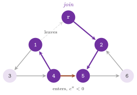
Algorithm 13.1 (Network simplex).
1  if the sum of the supplies has the wrong sign for the supply type:
   return INFEASIBLE; move the lower bounds into the supplies
2  T := tree of the artificial arcs from and to the root; set the flows,
   the potentials and the thread of T
3  make the heuristic initial pivots (see below)
4  while the pivot rule finds an eligible arc e:
5      w := join node of the ends of e in T
6      delta := largest amount around the cycle of e and T;
       f := last arc of the cycle, from w in the direction of the flow,
       to reach a bound (f = e if e reaches its other bound first)
7      if delta is infinite: go to 12
8      send delta around the cycle; if f != e: T := T - f + e
9      update the potentials of the side that f splits off, or of the rest
10 if some artificial arc that may carry no flow carries some: INFEASIBLE
11 put the lower bounds back, shift the potentials; return OPTIMAL
12 solve the problem again with zero costs: if it is infeasible, return
   INFEASIBLE; otherwise solve it again with its costs: return UNBOUNDED
Step 6 is findLeavingArc(), which scans the two sides of the cycle with a
strict and a weak comparison so as to keep the last blocking arc, and step 9
is updatePotential(). Step 10 checks the flow against \(\epsilon_f\), step 11
is the end of start(), and step 12 is feasibleUnbounded(). When the
supplies sum to zero, step 11 shifts the potentials so that their largest
value is at most zero under GEQ, and their smallest at least zero under LEQ,
as (13.5) requires.
Lemma 13.1. Let the subtree moved by a pivot be the part of the new tree hanging from the end \(u\) of the entering arc that was split off by the leaving arc, and let \(\sigma\) be the change of \(\pi(u)\) that makes the entering arc's reduced cost zero. Adding \(\sigma\) to the potentials of the subtree, or subtracting \(\sigma\) from those of all the other nodes, gives potentials under which every arc of the new tree has a zero reduced cost.
Proof. The arcs of the new tree are those of the old tree other than \(f\), which have a zero reduced cost and either both ends in the subtree or both ends outside it, together with the entering arc, which joins the two parts. Adding the same constant to the potentials of one part leaves the reduced costs of the arcs within each part unchanged, and \(\sigma\) makes the reduced cost of the entering arc zero; subtracting \(\sigma\) from the other part changes all the potentials by the constant \(-\sigma\) with respect to the first choice. \(\square\)
The code takes the second choice when the subtree holds more than half of the
\(n+1\) nodes, provided that the potential of the root stays within \(M/2\) of
zero for an exact Cost (within \(M\) otherwise). At the end,
alignPotential() shifts all the potentials so that the one of the root is
zero again. The next theorem gives the correctness of the answers; we assume,
as holds by construction in floating point and for an exact Cost whenever
\(nK\) is below half of its largest value, that \(M>nK\).
Theorem 13.3. (Correctness of NetworkSimplex.) Suppose that the pivots end. If no arc is eligible, then the problem is infeasible if and only if some artificial arc of cost \(M\) carries flow, and otherwise the flow and the shifted potentials satisfy (13.5) for the supply type. If a pivot has an infinite amount, its cycle is a cycle of negative cost made of arcs of \(G\) of infinite upper bound, and the answer of step 12 is right.
Proof. Let \(c_0\) be the costs with zero on the arcs of cost \(M\), and \(c_1\) the costs with one on those arcs and zero elsewhere, so that the cost of every arc is \(c_0+Mc_1\). By the linearity of the system that defines them, the tree potentials are \(\pi=\pi_0+My\), where \(\pi_0\) and \(y\) are the tree potentials for \(c_0\) and \(c_1\) with the root at zero. Each tree path from the root contains at most one arc of cost \(M\); hence, \(y\) takes the values \(-1\), \(0\) and \(1\). The difference \(\pi_0(u)-\pi_0(v)\) is the cost of the tree path between \(u\) and \(v\), whose arcs of nonzero cost are arcs of \(G\), at most \(n-1\) of them; hence, the reduced cost of each arc under \(\pi_0\) for \(c_0\) is at most \(nK<M\) in absolute value. Therefore, if the reduced cost of an arc under \(y\) for \(c_1\) is nonzero, i.e., at least 1 in absolute value, it decides the sign of its reduced cost under \(\pi\). If no arc is eligible, the nonbasic arcs at the lower bound have nonnegative reduced costs and those at the upper bound nonpositive ones, both under \(\pi\) and, by the remark above, under \(y\) for \(c_1\), while the tree arcs have zero reduced costs under both. By Theorem 13.1 (equality form), the flow minimizes the total flow on the arcs of cost \(M\) in the auxiliary problem. The original problem is feasible if and only if that minimum is zero, since the arcs of cost zero take exactly the slack of the GEQ or LEQ constraints; in the balanced case the conservation at the root forces the remaining artificial arcs to zero as well. This proves the first part. If the minimum is zero, the flow is optimal for the auxiliary problem by Theorem 13.1, and its restriction to \(G\), with the lower bounds put back, is optimal for the original one. Under GEQ with unbalanced supplies the arcs \(ru\) of cost zero have a nonnegative reduced cost, \(\pi(r)-\pi(u)\geq 0\), which is zero when they carry flow, i.e., when the constraint of \(u\) is slack; with \(\pi(r)=0\) this is (13.5), and LEQ is symmetric, while in the balanced case the shift of step 11 gives the signs. Finally, an infinite amount means that every arc of the cycle is traversed forward and has an infinite capacity, and that its cost is negative, since the entering arc is eligible. A cycle through the root would traverse forward an arc out of the root and an arc into it. One of them has cost \(M\) (under GEQ the arcs into the root, under LEQ and in the balanced case those out of it), and the cycle would cost at least \(M-nK>0\). Hence, the cycle lies in \(G\). If the problem is feasible, it is unbounded along this cycle; whether it is feasible is decided in step 12 by the same method on zero costs, which is never unbounded, and if it is, the run with the costs repeats the same pivots and ends unbounded again. \(\square\)
The termination of the pivots rests on the rule of step 6. A tree is strongly feasible if a positive amount of flow can be sent from each node to the root along its tree path within the bounds. The rule that takes the last blocking arc of the cycle, traversed from the join node in the direction of the flow, is due to Cunningham 1976.
Theorem 13.4. (Termination.) If the initial tree is strongly feasible, the tree stays strongly feasible after each pivot, no basis is repeated, and the method ends after finitely many pivots. The initial tree of the class is strongly feasible for every supply type.
Proof sketch. The first statement is the theorem of Cunningham 1976; see also Ahuja, Magnanti and Orlin 1993, §11.5. Its main step is that, after a pivot with the last blocking arc, every node of the new tree can again send a positive amount to the root. In a degenerate pivot the subtree that moves is then the one on the far side of the leaving arc, whose potentials all change in the same direction. Hence, a nondegenerate pivot strictly decreases the cost, a degenerate one strictly changes the sum of the potentials in a fixed direction, and the pair (cost, sum of potentials) never repeats. For the second statement, in the initial tree an arc \(ur\) carries \(sup(u)\geq 0\) towards the root and has an infinite capacity, while an arc \(ru\) carries \(-sup(u)\), which can be decreased if it is positive. In the balanced case and under LEQ the arcs \(ru\) are those of the nodes of negative supply. Under GEQ they are those of the nodes of negative supply as well, a node of zero supply hanging on an artificial arc \(ur\) of cost \(M\) and flow zero, which can be increased, with the arc \(ru\) of cost zero out of the tree at its lower bound. The heuristic initial pivots use the same rule. \(\square\)
We remark that the header states no bound on the number of pivots, and that the pivot rules of the class are not known to be polynomial. Each pivot costs the search of the rule, plus time proportional to the length of the cycle and to the size of the smaller part of the tree. In practice the method is usually the fastest one of the library on graphs of up to some thousands of nodes and on dense graphs (cf. section 13.9).
In step 3 the initial pivots are a heuristic of the original code. With a
single supply node and a single demand node, they are made on the arcs found
by a search backwards from the demand node over the arcs whose capacity is at
least the total supply; with more nodes, on the cheapest arc into each demand
node (or, under GEQ with less supply than demand, the cheapest arc out of each
supply node). Each of these arcs enters the basis if it is eligible. Also, the
constructor takes the flag arc_mixing, true by default, which stores the
arcs in an interleaved order, with a stride of \(\max\{\lfloor m/n\rfloor,3\}\),
rather than in the order of the digraph. According to the header, this usually
performs like the original order, but it makes the method more reliable and,
in special cases, significantly faster.
abLEMON
The potentials are updated on the smaller side of the tree at each pivot
(version 1.4.0). In floating point, the leaving arc goes to the bound it
is nearer to, its flow being set to that bound, rather than to the upper
bound for a flow of, e.g., \(10^{-16}\) (version 1.9.0), which may change
the sequence of pivots. A problem is answered UNBOUNDED only after a
check of its feasibility (version 1.4.1). Under GEQ with supplies of sum
below zero, LEMON 1.3.1 hung a node of zero supply on an arc \(ru\) of flow
zero, which made the initial tree not strongly feasible; no test observes
the difference, since no instance is known on which the pivot rules of
the class cycle from that tree.
13.4.2 Pivot rules¶
The argument of run() is the rule that chooses the entering arc, i.e., a
constant of the nested enum PivotRule. The arcs are scanned in a wraparound
fashion from where the last search stopped, and an arc is eligible when its
reduced cost, signed by its state, is below \(-\epsilon_c\). Let \(m'\) be the
number of arcs searched, i.e., those of the digraph and, when the supplies do
not sum to zero, also the second artificial arcs; the five rules are then as
follows.
FIRST_ELIGIBLEtakes the next eligible arc after the last one taken.BEST_ELIGIBLEtakes the most violating arc among all of them.BLOCK_SEARCH, the default, scans blocks of \(b=\max\{\lfloor\sqrt{m'}\rfloor, 10\}\) arcs and stops at the end of the first block after which an eligible arc has been seen, taking the most violating arc scanned.CANDIDATE_LISTbuilds, in a major iteration, a list of at most \(\ell=\max\{\lfloor 0.25\sqrt{m'}\rfloor, 10\}\) eligible arcs, and then takes the best arc of the list, dropping those no longer eligible, in at most \(\max\{\lfloor 0.1\,\ell\rfloor, 3\}\) minor iterations.ALTERING_LISTkeeps the \(h=\max\{\lfloor 0.01\,b\rfloor, 3\}\) best candidates of the previous iteration that are still eligible, and extends them by blocks of \(b\) arcs until the list has more than \(h\) arcs after the first block, or any after a later one; it takes the best arc and keeps the next \(h\) best.
Each rule is a private class of NetworkSimplex (FirstEligiblePivotRule,
BestEligiblePivotRule, BlockSearchPivotRule, CandidateListPivotRule and
AlteringListPivotRule), which run() instantiates for the chosen rule, and
whose constants are those given above. According to the header, BLOCK_SEARCH
and ALTERING_LIST were the most efficient rules on the instances on which
they were tested, and BLOCK_SEARCH, being simpler and somewhat more
reliable, was made the default. Any rule takes an eligible arc whenever there
is one, which is all that Theorems 13.3 and 13.4 need.
13.5 The starting flow and the infinite bounds¶
The other three classes work on a residual network, in which each arc of the
digraph appears forward and backward. An extra root node is joined to the
nodes by a pair of arcs, which under GEQ take the unmet demand, with no cost
and a capacity of one more than the deficit of the supplies. Two functions of
lemon/bits/mcf_feasible_flow.h prepare that network.
The first one, feasibleFlow(), finds the flow that CostScaling and
CycleCanceling start from, i.e., a flow within the bounds that meets the
supplies. It runs the push-relabel algorithm of Circulation (Algorithm 12.4
of chapter 12), with the active node of highest level
first, all the nodes at level zero at the start, a push towards any lower
level, and the first empty level as the proof that no such flow exists
(Goldberg and Tarjan 1988;
Cherkassky and Goldberg
1997). Its starting point is
the greedy flow of Circulation, in which each arc takes the deficit of its
head within its bounds. Theorem 12.6 applies to it word for word. Hence, it
ends, and when it fails the node being lifted, together with the nodes above
the empty level, form a set that no residual arc leaves and whose excess is
positive; this set of positive violation proves the problem infeasible, and
chapter 14 uses it as a certificate. In floating
point, an excess or a residual capacity within \(\epsilon_f\) counts as zero,
and at the end the residual capacities within it are moved to the reverse
arcs, lest the algorithms send round-off around.
The second function, infiniteBound(), gives the bound that replaces an
infinite upper bound in CostScaling and CycleCanceling (on every arc of
infinite upper bound) and in CapacityScaling (on the arcs of infinite upper
bound and negative cost, which it saturates at the start), namely
beyond the lower bound of the arc. If this does not fit the sums of the flows
over the \(k\) replaced arcs, the bound is cut to the largest value of Value
divided by \(k+2\). Whether a cycle of negative cost is made of arcs of infinite
upper bound is decided beforehand by negativeInfiniteCycle(), a Bellman-Ford
algorithm restricted to those arcs and run from a virtual node joined to all
the nodes. It runs only if one of those arcs has a negative cost, and it
reports a cycle if a distance still improves after \(n\) rounds; if such a cycle
exists, a feasible problem is answered UNBOUNDED. In floating point a cost,
and an improvement of a distance, count only beyond \(\epsilon_c\), as in the
operation traits of the algorithm of Bellman and Ford of section 13.8: a cycle
whose cost is zero in decimal but whose sum rounds a few units in the last
place below zero is then a cycle of cost zero, and the problem is answered
OPTIMAL, as by NetworkSimplex.
abLEMON
LEMON 1.3.1 answered UNBOUNDED with CostScaling and CycleCanceling
on any arc of negative cost and infinite upper bound, and the exact
comparisons of negativeInfiniteCycle() (version 1.4.1) gave the same
answer, with CapacityScaling too, on a cycle of costs \(-0.1\), \(-0.2\) and
\(0.3\) that NetworkSimplex solves; checkZeroInfiniteCycle() of
test/min_cost_flow_test.cc checks this cycle.
Theorem 13.5. (The finite bound.) Suppose that (13.1) is feasible and that no cycle of negative cost is made of arcs of infinite upper bound. Replace the infinite upper bound of some arcs by their lower bound plus \(B\), and let \(f^*\) and \(\pi^*\) be an optimal flow and optimal potentials of the problem so obtained. Then \(f^*\) and \(\pi^*\) are optimal for the original problem.
Proof. The original problem is bounded, since an unbounded direction of the polyhedron of the flows would be a nonnegative combination of cycles of infinite capacity, one of them of negative cost; hence, it has an optimal basic solution \(f_0\) (the polyhedron has vertices, the flows being bounded below). In a basic solution of the auxiliary problem of section 13.4 the nonbasic arcs are at a finite bound, an arc of infinite upper bound being nonbasic at its lower bound. The flow of a tree arc is then the supply of the side of the tree that it separates from the root, plus or minus the flows of the nonbasic arcs between the two sides. Hence, for each arc \(a\), \(|f_0(a)|\leq\sum_u|sup(u)|+\sum_{b\neq a}(|lower(b)|+|upper(b)|)\), where the infinite upper bounds are left out, and \(f_0(a)-lower(a)\leq B-1<B\). Thus, \(f_0\) is feasible for the problem with the bounds replaced, which has therefore the same optimal value, and \(f^*\) is optimal for the original problem. By the complementary slackness between \(\pi^*\) and \(f_0\) in the replaced problem, an arc whose bound was replaced and whose reduced cost under \(\pi^*\) is negative would carry \(lower+B\) in \(f_0\), which is false; hence, \(cost^{\pi^*}\geq 0\) on those arcs, and \(\pi^*\) with \(f^*\) satisfies (13.5) for the original bounds. \(\square\)
13.6 Cost scaling¶
CostScaling implements the cost scaling algorithm of Goldberg and Tarjan
(Goldberg and Tarjan 1990;
Goldberg 1997; Bünnagel, Korte
and Vygen 1998), a primal-dual
method that one may regard as the generalization to costs of the push-relabel
algorithm of Preflow. On the residual network with the root, a flow \(f\)
(with excesses allowed) and potentials \(\pi\) are \(\varepsilon\)-optimal when
and \(\varepsilon=0\) gives back the conditions of Theorem 13.2. The class
multiplies the costs by \((n+1)\alpha\), where \(\alpha\) is the scaling factor,
i.e., the argument factor of run() (16 by default, at least 2, as it
asserts), and works on these scaled costs. It starts from \(\varepsilon\) equal
to the largest scaled cost of a residual arc divided by \(\alpha\) and from zero
potentials, and it divides \(\varepsilon\) by \(\alpha\) after each phase. In a
phase it refines the flow. First it saturates the residual arcs of negative
reduced cost, which makes the flow \(0\)-optimal but creates excesses and
deficits. Then it removes them by pushes along the admissible arcs, i.e.,
those of negative reduced cost, and by relabels, each of which lowers the
potential of a node \(u\) by \(c_u+\varepsilon\), where \(c_u\) is the least reduced
cost of the residual arcs out of \(u\).
Algorithm 13.2 (Cost scaling).
1  find a feasible flow f (section 13.5); if none: return INFEASIBLE
2  if a cycle of infinite capacity has negative cost: return UNBOUNDED
3  scale the costs by (n+1) alpha; eps := largest scaled cost / alpha;
   pi := 0
4  while eps >= eps_min:
5      from the second phase on: price refinement; if it proves the flow
       eps-optimal: skip to 9
6      saturate the residual arcs of negative reduced cost
7      while some node u has positive excess (FIFO order):
           push or augment along admissible arcs, or relabel u;
           every few relabels, make a global update of the potentials
8      (the flow is now eps-optimal and has no excess)
9      eps := eps / alpha, or eps_min if eps lies in (eps_min, alpha eps_min)
10 divide the potentials by (n+1) alpha; if some residual arc has a
   reduced cost below -eps_c, correct them by Bellman-Ford
11 shift the potentials so that the largest is zero; return OPTIMAL
The nested enum Method selects the operation of step 7. With PUSH the flow
moves on one admissible arc at a time, with a look-ahead that avoids pushing
into a node that would only send the flow back. With AUGMENT it moves along
admissible paths from a node with excess to a node with deficit. With
PARTIAL_AUGMENT, the default and, according to the header, the most
efficient and reliable one, it moves along admissible paths of at most 4 arcs.
Two heuristics of Goldberg 1997
are applied. The price refinement of step 5 computes potentials that may prove
the current flow \(\varepsilon\)-optimal before any push. The global update of
step 7 recomputes the potentials by a bucket-based search from the deficits,
after a number of relabels equal to \(n+1+s^2\) with AUGMENT and
PARTIAL_AUGMENT and to twice that with PUSH, \(s\) being the number of nodes
of positive supply net of the lower bounds. Both change only the potentials,
and keep (13.8).
Lemma 13.2. Step 6 makes the flow \(0\)-optimal, and each push and each relabel of step 7 keeps it \(\varepsilon\)-optimal.
Proof. After step 6 an arc of negative reduced cost is saturated, and its reverse, the only arc that step 6 adds, has a positive reduced cost. A push along an admissible arc \(uv\) may add the arc \(vu\), whose reduced cost \(-cost^\pi(uv)\) is positive. A relabel of \(u\) subtracts \(c_u+\varepsilon\) from \(\pi(u)\), where \(c_u\geq-\varepsilon\) by (13.8); an arc out of \(u\) of reduced cost \(c\geq c_u\) gets \(c-c_u-\varepsilon\geq-\varepsilon\), and an arc into \(u\) gets \(c+c_u+\varepsilon\geq c\). \(\square\)
Lemma 13.3. With an integer LargeCost, a
feasible flow that is \(1\)-optimal for the scaled costs is optimal; the final
correction of step 10 gives potentials that, with the shift of step 11,
satisfy (13.5).
Proof. A cycle \(W\) of the residual network has at most \(n+1\) arcs, and its scaled cost is the sum of its reduced costs, at least \(-(n+1)\); its original cost is therefore at least \(-1/\alpha>-1\), and it is an integer, hence nonnegative. By Theorem 13.2 (on the network with the root, in the equality form) the flow is optimal. The Bellman-Ford algorithm on the reduced costs of the residual arcs, from a virtual node, then finds no negative cycle, and adding its distances to the potentials makes every residual reduced cost nonnegative, as in Theorem 13.2. Under GEQ with unbalanced supplies, the arcs from the root to the nodes are always residual, since their capacity exceeds the unmet demand; hence, the root has the largest potential. Its arc to a node with unmet demand is residual in both directions, and that node has the same potential; after the shift of step 11 these are the conditions of (13.5) on the nodes. \(\square\)
Theorem 13.6. (Cost scaling.) On integer data
CostScaling returns the right answer, and with OPTIMAL an optimal flow and
potentials meeting (13.5). As stated in the header, its worst case running
time is \(O(n^2m\log(nK))\).
Proof sketch. The answers INFEASIBLE and UNBOUNDED follow from section
13.5 (the starting flow, Theorem 12.6, and negativeInfiniteCycle()), and the
answer OPTIMAL from Lemmas 13.2 and 13.3 and from Theorem 13.5 for the
replaced infinite bounds, provided that each refinement ends. The refinement
ends by the analysis of Goldberg and Tarjan
1990: a node with excess has a
residual path to a node with deficit, along which the reduced costs of an
\(\alpha\varepsilon\)-optimal flow bound the drop of its potential. Hence, each
node is relabeled \(O(n)\) times per phase (for a fixed \(\alpha\)), with \(O(nm)\)
saturating and \(O(n^2m)\) other pushes, and the refinement takes \(O(n^2m)\) time
in its generic form. The number of phases is \(O(\log_\alpha((n+1)\alpha
K))=O(\log(nK))\). See also Ahuja, Magnanti and Orlin 1993,
§10.3. \(\square\)
We remark that the bound is that of the generic method, whose operations the
three methods of the class implement in different orders, and that the scaled
costs \((n+1)\alpha\,cost\) must fit in LargeCost. For the internal
computations the class uses the type LargeCost of the traits class
CostScalingDefaultTraits< GR , V , C >, which also defines Digraph,
Value and Cost: LargeCost is long long for an integer Cost (or
long without LEMON_HAVE_LONG_LONG) and double otherwise. The named
parameter SetLargeCost< T > changes it, provided that Cost is convertible
to T, and the class names the traits Traits and the type LargeCost. The
last value \(\varepsilon_{min}\) of the scaling is 1 for an integer LargeCost,
which proves the flow optimal by Lemma 13.3, and otherwise
\(\epsilon_c\,(n+1)\,\alpha\), i.e., the tolerance on the reduced costs in the
scaled units, which the final flow then meets. In practice the method is
typically the most efficient one of the library on large sparse graphs (cf.
section 13.9).
abLEMON
CostScaling finds its starting flow on its residual network (version
1.4.0), where LEMON 1.3.1 ran Circulation on the digraph, and it takes
floating-point costs, capacities and supplies (version 1.6.0). The price
refinement of LEMON 1.3.1 could write past the end of its buckets, which
is fixed.
13.7 Capacity scaling¶
CapacityScaling implements the capacity scaling version of the successive
shortest path algorithm (Edmonds and Karp
1972; Ahuja, Magnanti and
Orlin 1993, chapter 10). It is a
dual method: it keeps potentials under which the residual arcs of capacity at
least \(\Delta\) have nonnegative reduced costs (the flow is
\(\Delta\)-optimal), and it sends flow from the nodes with excess to the nodes
with deficit along shortest paths. Under GEQ with unbalanced supplies the root
starts with the excess \(-\sum_u sup(u)\), which it may send to any node at no
cost, i.e., it supplies the unmet demand.
Algorithm 13.3 (Capacity scaling).
1  saturate the arcs of negative cost (an infinite bound replaced by B,
   section 13.5); Delta := largest power of 2 (times the unit) not above
   the smallest of the largest excess, deficit and residual capacity
2  loop:
3      saturate the residual arcs with r >= Delta and reduced cost < -eps_c
4      while a node s has e(s) >= Delta and some node has e <= -Delta:
5          Dijkstra from s on the arcs with r >= Delta, until a node t
           with e(t) <= -Delta is settled
6          if none is reached: (at the last Delta) return INFEASIBLE,
           (otherwise) go on with the next node s
7          augment along the path by min{ e(s), -e(t), its capacities }
8          update the potentials of the settled nodes: pi += dist - dist(t)
9      if Delta = unit: return OPTIMAL (or UNBOUNDED, section 13.5)
10     Delta := Delta / factor, or unit if Delta <= factor unit
Here the unit is 1 for an exact Value and \(\epsilon_f\) otherwise; hence, in
floating point the last phase sends any amount above the tolerance. With a
factor of at most 1, or when the initial \(\Delta\) is already the unit, the
scaling is disabled, and the method becomes the plain successive shortest path
algorithm, which is usually the fastest choice when the supplies and the
capacities are small. In the end the potentials are shifted so that the root
has potential zero.
Lemma 13.4. Steps 3, 7 and 8 keep the flow \(\Delta\)-optimal, and after step 8 the arcs of the path found have a zero reduced cost.
Proof. Step 3 saturates the arcs that violate the condition, whose reverses get a positive reduced cost. In step 5 the distances \(dist\) are computed on the nonnegative reduced costs; a settled node \(u\) has \(dist(u)\leq dist(t)\), and an unsettled node \(v\) has a true distance at least \(dist(t)\). After step 8, an arc between two settled nodes has the reduced cost \(cost^\pi(uv)+dist(u)-dist(v)\geq 0\), which is zero along the shortest path tree. An arc from a settled \(u\) to an unsettled \(v\) has \(cost^\pi(uv)+dist(u)-dist(t)\geq 0\), since \(dist(v)\leq dist(u)+cost^\pi(uv)\) and \(dist(v)\geq dist(t)\), and an arc into a settled node from an unsettled one does not decrease its reduced cost. The augmentation of step 7 moves at least \(\Delta\) along arcs of zero reduced cost, whose reverses then have a zero reduced cost too. \(\square\)
Theorem 13.7. (Capacity scaling.) On integer
data CapacityScaling returns the right answer, and with OPTIMAL an optimal
flow and potentials meeting (13.5). As stated in the header, its worst case
running time is \(O(m\log U\,(n+m)\log n)\), under the assumption recalled
below.
Proof. In the last phase (\(\Delta=1\)) every residual arc has a residual
capacity of at least 1. If the phase ends with OPTIMAL, no node has an
excess of 1 or more; since the excesses are integers and sum to zero, all of
them are zero, and the flow is feasible. By Lemma 13.4 every residual arc then
has a nonnegative reduced cost, so that the flow is optimal by Theorem 13.2
(with Theorem 13.5 for the arcs saturated at \(B\)), and the potentials meet
(13.5) by the argument of Lemma 13.3. If the phase ends with INFEASIBLE, the
set \(R\) of the nodes that the search reached from \(s\) is closed in the
residual network and holds no node of negative excess, while \(e(s)>0\). If \(R\)
does not hold the root, the excesses of \(R\) sum, as in the proof of Theorem
12.6, to the violation of \(R\) in (12.6), which is then positive. If it does,
\(R\) holds every node, since the arcs from the root are residual; then no node
has a deficit, which contradicts the zero sum of the excesses. For the running
time, there are \(\lceil\log U\rceil+1\) phases, and each search takes
\(O((n+m)\log n)\) time with a heap. By the analysis of Ahuja, Magnanti and
Orlin 1993, §10.2, a phase makes
\(O(m)\) augmentations, each of at least \(\Delta\), since the excesses left by
the previous phase and the saturations of step 3 sum to \(O((n+m)\Delta)\).
\(\square\)
We remark that this count of the augmentations assumes, as the model of that
analysis does, that a node of excess at least \(\Delta\) reaches a node of
deficit at least \(\Delta\) in the residual network of the arcs of capacity at
least \(\Delta\). The code skips a node that does not, until a smaller \(\Delta\),
which the count does not cover. In the searches the class uses the heap type
Heap of the traits class CapacityScalingDefaultTraits< GR , V , C > (which
also defines Digraph, Value and Cost), by default
QuadHeap< Cost , RangeMap< int > >, whose fewer levels make the searches
cheaper than on a binary heap (Johnson
1975). The named parameter
SetHeap< T > replaces it by any heap that meets the concept of chapter
7 with the priority type Cost and the cross reference map
RangeMap< int >, and the class names the traits Traits and the heap
Heap.
abLEMON
The default heap is a 4-ary heap (version 1.4.0), the class compiles on
value types narrower than int, and it takes floating-point data (version
1.6.0).
13.8 Cycle canceling¶
CycleCanceling implements three cycle canceling methods (Klein
1967; Goldberg and Tarjan
1989), which start from the
feasible flow of section 13.5 and cancel cycles of negative cost of the
residual network until none is left, i.e., until the flow is optimal by
Theorem 13.2. The nested enum Method selects one of them.
SIMPLE_CYCLE_CANCELINGruns rounds of the algorithm of Bellman and Ford on the residual network, from a virtual node, with a limit on the number of rounds that starts at 2 and grows by a factor of 1.5 when no cycle is found; after each batch of rounds it cancels the node-disjoint cycles of the graph of the predecessors. It stops when a round improves no distance within the limit.MINIMUM_MEAN_CYCLE_CANCELINGcancels a cycle of minimum mean cost at each step, found by Howard's algorithm with a limit of \(\max\{n,5\}\) iterations and, if the limit is reached, by the strongly polynomial algorithm of Hartmann and Orlin (chapter 16); it stops when the minimum mean is not below \(-\epsilon_c\).CANCEL_AND_TIGHTEN, the default, which the header calls by far the most efficient and reliable, is the improved version of the previous method of Goldberg and Tarjan 1989.
In Cancel-and-Tighten an arc is admissible when its reduced cost is negative. A phase cancels, by a depth first search, the cycles of admissible arcs, until the admissible network is acyclic. Then it tightens the potentials along a topological order of that network, and it recomputes \(\varepsilon\) as the largest value of \(-cost^\pi\) on the residual arcs. Every \(\max\{\lfloor\sqrt{n+1}\rfloor,5\}\)-th phase, instead, sets \(\varepsilon\) to the opposite of the minimum cycle mean of the residual network, and recomputes the potentials from it by the algorithm of Bellman and Ford on the costs shifted by the mean.
Algorithm 13.4 (Cancel-and-Tighten).
1  find a feasible flow f (section 13.5); if none: return INFEASIBLE
2  if a cycle of infinite capacity has negative cost: return UNBOUNDED
3  pi := 0; eps := largest -cost(uv) over the residual arcs
4  while eps * (n+1) >= 1 (exact costs), or eps > eps_c (floating point):
5      cancel the cycles of admissible arcs (cost^pi < 0) by DFS
6      if this is not the k-th phase:
7          tighten pi along a topological order of the admissible arcs;
           eps := largest -cost^pi(uv) over the residual arcs
8      else:
9          eps := - (minimum cycle mean of the residual network);
           pi := potentials for eps, by Bellman-Ford
10 compute the final potentials by Bellman-Ford; return OPTIMAL
During the phases the potentials are double, fractional even with an exact
Cost, and the test of admissibility uses a tolerance of
\(\min\{10^{-6},1/(2(n+1))\}\) then, i.e., \(10^{-6}\) as in LEMON 1.3.1 up to
about \(5\cdot 10^5\) nodes, and \(\epsilon_c\) with a floating-point Cost.
After the last phase of the two methods based on mean cycles, the potentials
are computed by the algorithm of Bellman and Ford on the residual network (in
SIMPLE_CYCLE_CANCELING its distances already give them). Its operation
traits count an improvement only beyond \(\epsilon_c\), since in floating point
the round-off of the sums can make a cycle of cost zero (e.g., an arc and its
reverse) look negative for ever.
Theorem 13.8. (Cycle canceling.) On integer
data each of the three methods ends, and with OPTIMAL it returns an optimal
flow and potentials meeting (13.5). The minimum mean cycle canceling makes
\(O(nm^2\log n)\) cancellations and runs in \(O(n^2m^3\log n)\) time, as the
header states, when each minimum mean cycle is found by the algorithm of
Hartmann and Orlin; for Cancel-and-Tighten the header states \(O(n^2m^2\log
n)\).
Proof. Each cancellation sends a positive integer amount around a cycle of
negative integer cost, and decreases the cost by at least 1. The problem with
the bounds of section 13.5 is bounded, so that there are finitely many
cancellations. SIMPLE_CYCLE_CANCELING stops only when a round of Bellman and
Ford improves no distance, i.e., when the residual network has no negative
cycle, and the minimum mean method stops when the minimum mean is nonnegative.
Cancel-and-Tighten stops when every residual arc has
\(cost^\pi\geq-\varepsilon\) with \(\varepsilon(n+1)<1\); then each residual
cycle, of at most \(n+1\) arcs, has a cost above \(-1\), hence nonnegative. While
\(\varepsilon(n+1)\geq 1\), an arc of reduced cost \(-\varepsilon\) is below
\(-1/(2(n+1))\) and is admissible; after the phase of the minimum cycle mean,
the arcs of a cycle of mean \(-\varepsilon\) all have reduced cost
\(-\varepsilon\), so that the next phase cancels it. In the three cases the flow
is optimal by Theorem 13.2, and Theorem 13.5 covers the replaced bounds. The
final distances of Bellman and Ford meet (13.5) by the argument of Lemma 13.3;
the root has potential zero, since every node is reached from it by a residual
arc of cost zero and every residual cycle through it has a nonnegative cost.
For the running time of the minimum mean method, see Goldberg and Tarjan
1989 and Ahuja, Magnanti and
Orlin 1993, §10.5: the opposite of
the minimum mean never grows, and it decreases by a factor of at least \(1-1/n\)
every \(m\) cancellations, which bounds their number by \(O(nm^2\log n)\), each
costing \(O(nm)\) for the cycle. Cancel-and-Tighten makes \(O(nm\log n)\) phases
by the analysis of Goldberg and Tarjan, each of which takes \(O(nm)\) for its
cancellations. \(\square\)
The class has no traits parameter, and the header warns that, in practice, the
method is typically orders of magnitude slower than the scaling algorithms and
NetworkSimplex.
abLEMON
CycleCanceling finds its starting flow on its residual network (version
1.4.0), takes floating-point data (version 1.6.0), and compares with zero
only through the tolerances, its inner minimum mean cycle searches
included (version 1.9.0). With an exact Cost, LEMON 1.3.1 took \(10^{-6}\)
as the tolerance of admissibility of Cancel-and-Tighten on any digraph,
which on more than about \(10^6\) nodes leaves a cycle of mean between
\(-10^{-6}\) and \(-1/(n+1)\) never admissible, and the method does not end
on a cycle of \(1.1\cdot 10^6\) nodes and cost \(-1\), which abLEMON solves
in some minutes, too long for a test of the library.
13.9 Choosing an algorithm¶
In the documentation of the module, which follows the experimental study of
Király and Kovács 2012,
NetworkSimplex and CostScaling are recommended as the most efficient
classes in general. NetworkSimplex is usually the fastest on relatively
small graphs (up to several thousands of nodes) and on dense graphs, while
CostScaling is typically more efficient on large graphs (e.g., hundreds of
thousands of nodes or more), especially sparse ones. Other classes may be
faster in special cases; e.g., when the total supply or the capacities are
rather small, CapacityScaling without scaling is usually the fastest. In our
view, CycleCanceling is mostly of interest for its strongly polynomial bound
and for teaching. We remark that these are statements about typical instances,
and that the ranking on a given family of problems is best found by running
the four classes on it, which their common interface makes easy (cf. section
13.2). Also, note that only NetworkSimplex takes the LEQ form directly.
13.10 Exercises¶
Exercise 13.1. Verify the identity (13.4), and
use it to show directly that a flow of (13.1) with a cycle of negative cost in
its residual network is not optimal. Then check (13.5) on the four answers of
manual/examples/13-min-cost-flow.cc, which does it in its function
optimal().
Exercise 13.2. Transform a problem in the LEQ
form (13.2) into the GEQ form with ReverseDigraph and NegMap, solve it
with CostScaling, and compare the cost with that of NetworkSimplex with
supplyType( LEQ ). (The supply types are checked by checkSupplyTypes() in
test/min_cost_flow_test.cc.)
Exercise 13.3. Solve the problem of
manual/examples/13-floating-point.cc with tolerances( 0 , 0 ) on supplies
that are exact in binary (e.g., \(0.25\), \(0.5\) and \(-0.75\)), and then on \(0.1\),
\(0.2\) and \(-0.3\) with the default tolerances; explain the difference by
(13.6). (The tolerances are checked by checkTolerances() and
checkToleranceGetters() in test/min_cost_flow_test.cc.)
Exercise 13.4. Time the five pivot rules of
NetworkSimplex on random instances of a few thousand nodes, on an idle
machine and with repeated runs, and compare the default with BEST_ELIGIBLE;
repeat with arc_mixing set to false.
Exercise 13.5. Run CostScaling with the three
methods and with the factors 2, 16 and 64, and CapacityScaling with the
factors 1 and 4, on the same instances, and check that the costs agree. (The
battery test/min_cost_flow_battery_test.cc runs every algorithm and method
on limit cases and random instances, with integer and floating-point data.)
Exercise 13.6. Compute the bound \(B\) of (13.7)
for the problem of manual/examples/13-min-cost-flow.cc with all the upper
bounds infinite, and verify that an optimal flow of that problem sends less
than \(B\) on each arc, as Theorem 13.5 asserts.