6. Searching¶
[Source: include/ADS/search/BinarySearch.h, MonotoneSearch.h,
InterpolationSearch.h, KnuthSearches.h, SortedSearches.h,
StaticSearch.h, CountLess.h, PGMIndex.h, CompressedPGMIndex.h,
DynamicPGMIndex.h, Minimum.h, LocalOptima.h, Selection.h,
NthElement.h, RangeMinimum.h, WordRangeMinimum.h]
We are concerned in this chapter with the questions that can be answered
on a vector by looking at few of its items: the place of a key in a
sorted vector, the minimum and the local optima, the item of a given rank,
and the minimum of any range of an array after a preprocessing. We first
treat the searches in a sorted vector, both in the forms of the textbooks
(§6.2) and in the forms that count the misses of
the cache and the branches that the processor mispredicts
(§6.3). Then come the learned indexes, which
replace the comparisons of the upper levels of a search by a model of the
keys, in the static, compressed and dynamic forms of the PGM-index
(§6.4 to §6.6). Finally, the
minimum and the local optima (§6.7), the
selection (§6.8) and the range minima
(§6.9) precede a comparison of the searches on
what each one is meant for (§6.10). In the sets of
§1.9, CompressedPGMIndex.h, CountLess.h,
DynamicPGMIndex.h, NthElement.h, RangeMinimum.h, StaticSearch.h and
WordRangeMinimum.h are advanced and the other headers of this chapter are
base.
6.1 Definitions and notation¶
We are given a vector \(A[ 0 .. n - 1 ]\) of items of a totally ordered
universe, compared by an order less() (the operator \(<\) unless one is
given); \(A\) is sorted if \(A[ i ] \le A[ i + 1 ]\) for each \(i\). A
comparison is the evaluation of the order on two items, and the cost of
a search is the number of its comparisons, the other operations being
proportional to it unless we say otherwise. We call rank of an item its
place in the sorted order, counted from 1 in Selection.h (as in
Montresor 2025, §17.1) and from 0
in NthElement.h and SortedSearches.h (as in the standard library). We
write \(A[ i .. j ]\) for the items of the places from \(i\) to \(j\), and
\(A[ i .. j )\) for those from \(i\) to \(j - 1\). Furthermore,
\(\mathrm{lowerBound}( v )\) is the first place of an item not smaller than
\(v\) (\(n\) if there is none), \(\mathrm{upperBound}( v )\) the first place of
an item larger than \(v\), and \(\mathrm{RMQ}( i , j )\), \(i \le j\), the
place of the leftmost minimum of \(A[ i .. j ]\). Finally, \(B\) is the number
of items in a line of cache of 64 bytes (e.g., 16 of 32 bits), and
\(\epsilon\) and \(\epsilon_r\) are the largest errors, in places, of the
lines of a learned index at its last level and at the others.
A comparison-based search is a decision tree (Montresor 2025, §2.7.4), i.e., a binary tree whose inner nodes are the comparisons and whose leaves are the answers. A run of the search is a path from the root to a leaf, and the worst case of the search is thus the height of its tree. Table 6.1 collects the searches of a key in a sorted vector.
Table 6.1. The searches of a key in a sorted
vector of ADS/search and their comparisons; \(h\) is the place of the
answer.
| Function | Comparisons | Source |
|---|---|---|
binarySearch() |
\(2 ( \lfloor \log_2 n \rfloor + 1 )\) at most | Montresor 2025, §1.2 |
lowerBound(), upperBound() |
\(\lceil \log_2 ( n + 1 ) \rceil\), as (6.1) | Montresor 2025, exercise 12.13 |
gallopSearch(), exponentialSearch() |
\(2 \lceil \log_2 ( h + 1 ) \rceil + O( 1 )\), as (6.3) | Bentley and Yao 1976 |
interpolationSearch() |
\(O( \log \log n )\) expected on uniform keys, \(O( n )\) in the worst case | Montresor 2025, §12.1; Perl et al. 1978 |
fibonacciSearch() |
about \(1.44 \log_2 n\) | Ferguson 1960; Knuth 1998 |
uniformBinarySearch() |
\(\lfloor \log_2 n \rfloor + 1\) at most | Knuth 1998 |
branchlessLowerBound() |
\(\lceil \log_2 n \rceil + 1\), none mispredicted | Khuong and Morin 2017 |
SPlusTree::lowerBound() |
\(H\) lines of (6.5) | Slotin 2022 |
PGMIndex::lowerBound() |
(6.6) | Ferragina and Vinciguerra 2020 |
6.2 Searching a sorted vector¶
The binary search of Montresor 2025,
§1.2 (binarySearch()) compares \(v\)
with the middle item \(A[ m ]\) of the part \(A[ i .. j ]\) still to examine, and
goes on in \(A[ i .. m - 1 ]\) if \(v < A[ m ]\) and in \(A[ m + 1 .. j ]\) if
\(v > A[ m ]\) (Algorithm 6.1). It stops as soon as it
meets \(v\), at the price of two comparisons per step, and returns \(-1\) when \(v\)
is not there; an overload calls a function trace( i , j , m ) at each step,
which prints the table of the example of the book. In the code, the middle is
computed as \(m = i + \lfloor ( j - i ) / 2 \rfloor\), which, unlike
\(\lfloor ( i + j ) / 2 \rfloor\), cannot overflow (the bug of
Arrays.binarySearch of Java until 2003). In turn, decisionTree() builds
the decision tree of the search as a BinaryTree that the caller owns (nil on
an empty vector), whose root is the middle item of the vector and whose
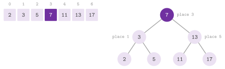
subtrees are the decision trees of the two halves (Figure
6.1).
Algorithm 6.1. The binary search (Montresor 2025, §1.2), the tail recursion of the book as a loop, and its decision tree.
Lemma 6.1. On a sorted vector of \(n\)
items, binarySearch() returns a place of \(v\) if \(v\) occurs and \(-1\)
otherwise, after at most \(2 ( \lfloor \log_2 n \rfloor + 1 )\)
comparisons. The tree of decisionTree() is a binary search tree whose
invisit is \(A\), of height \(\lfloor \log_2 n \rfloor\) for \(n \ge 1\), whose
levels \(0 , \ldots , \lfloor \log_2 ( n + 1 ) \rfloor - 1\) are full; hence
all its levels are full but the last one.
Proof. If \(v\) occurs, it occurs in \(A[ i .. j ]\): this holds at the start, and a step that finds \(A[ m ] < v\) (or \(v < A[ m ]\)) leaves out \(A[ i .. m ]\) (or \(A[ m .. j ]\)), whose items are all smaller (or larger) than \(v\), since \(A\) is sorted. Its steps visit the nodes of a path of the decision tree from its root, since the tree of \(A[ i .. j ]\) has the root \(A[ m ]\) and the subtrees of \(A[ i .. m - 1 ]\) and \(A[ m + 1 .. j ]\); each step makes at most two comparisons, and the path has at most as many nodes as the height plus one. In the tree of \(A[ i .. j ]\), the invisit is that of the left subtree, \(A[ m ]\) and that of the right one, i.e., \(A[ i .. j ]\) by induction, and a tree whose invisit is sorted is a search tree. On \(n \ge 2\) items the subtrees have \(\lfloor ( n - 1 ) / 2 \rfloor\) and \(\lceil ( n - 1 ) / 2 \rceil = \lfloor n / 2 \rfloor\) items; by induction the height is \(1 + \lfloor \log_2 \lfloor n / 2 \rfloor \rfloor = \lfloor \log_2 n \rfloor\), and the number of full levels is \(1 + \lfloor \log_2 ( \lfloor ( n - 1 ) / 2 \rfloor + 1 ) \rfloor = 1 + \lfloor \log_2 \lfloor ( n + 1 ) / 2 \rfloor \rfloor = \lfloor \log_2 ( n + 1 ) \rfloor\), the smaller subtree deciding it. Since \(\lfloor \log_2 ( n + 1 ) \rfloor \ge \lfloor \log_2 n \rfloor\), only the last level may not be full. \(\square\)
The height of the tree is thus the worst case of the search, in steps.
Lemma 6.2. Each comparison-based search for the place \(\mathrm{lowerBound}( v )\) in a sorted vector of \(n\) items makes, in the worst case, at least
comparisons.
Proof. Each of the \(n + 1\) places \(0 , \ldots , n\) is the answer for some \(v\), and the decision tree of the search has therefore at least \(n + 1\) leaves. A binary tree of height \(h\) has at most \(2^h\) leaves, whence (6.1). \(\square\)
lowerBound() meets (6.1), and upperBound() is the same search with the
test reversed; their difference is the number of the occurrences of \(v\)
(Montresor 2025, exercise 12.13;
Algorithm 6.2). Both take any order less(), and
lowerBound() also searches a range \([ \mathit{lo} , \mathit{hi} )\) of
the vector, which the other searches of the chapter call.
Algorithm 6.2. The lower bound and the upper bound (Montresor 2025, exercise 12.13).
Lemma 6.3. lowerBound() keeps the
invariant
with \(A[ -1 ] = -\infty\) and \(A[ n ] = +\infty\), and returns \(\mathrm{lowerBound}( v )\) after at most \(\lceil \log_2 ( n + 1 ) \rceil\) comparisons.
Proof. (6.2) holds at the start, with \(\mathit{lo} = 0\) and \(\mathit{hi} = n\). A comparison of \(v\) with \(A[ m ]\) moves \(\mathit{lo}\) to \(m + 1\) when \(A[ m ] < v\) and \(\mathit{hi}\) to \(m\) otherwise, which keeps (6.2) since \(A\) is sorted. Each step takes the length \(\ell = \mathit{hi} - \mathit{lo}\) to at most \(\lfloor \ell / 2 \rfloor\); the loop thus ends after at most \(\lfloor \log_2 n \rfloor + 1 = \lceil \log_2 ( n + 1 ) \rceil\) comparisons with \(\mathit{lo} = \mathit{hi}\), which is the answer by (6.2). \(\square\)
Its contracts check (6.2) at the result, and that the range is sorted, an audit that costs \(O( n )\) against the \(O( \log n )\) of the search.
When the answer \(h\) is near the start, or the length of the vector is not
known, the search of Bentley and Yao 1976
doubles a bound before the binary search (gallopSearch(), exercise 12.9
of Montresor 2025, and
exponentialSearch() and unboundedSearch() of MonotoneSearch.h). Its probes at the places \(0 , 1 , 3 , 7 , \ldots , 2^k - 1\) stop at the first
\(k\) with \(A[ 2^k - 1 ] \ge v\), i.e., \(k = \lceil \log_2 ( h + 1 ) \rceil\),
after \(k + 1\) comparisons. In gallopSearch() the binary search that
follows runs on the places \(2^{k-1}\) to \(2^k - 2\), \(2^{k-1} - 1\) of them,
since the place \(2^k - 1\) is already known to hold an item not smaller
than \(v\), and so costs at most \(k - 1\) more comparisons
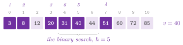
(Algorithm 6.3 and
Figure 6.2). In all, for \(h \ge 1\), at most
comparisons (1 for \(h = 0\)), which depend on the answer but not on \(n\) (Lemma 6.4). Bentley and Yao 1976 also show that applying the same idea to the search of \(k\) gives \(\log_2 h + \log_2 \log_2 h + \cdots\) comparisons, close to the lower bound \(\log_2 h\).
Algorithm 6.3. The searches with a bound that doubles (Bentley and Yao 1976): on a sorted vector, on a predicate \(p\) false and then true on the integers, and on a sequence of unknown length.
exponentialSearch() finds the least \(i \ge \mathit{lo}\) at which a predicate
\(p\), false and then true, holds (the method \(B_1\) of Bentley and Yao). Its
binary search too leaves out the last probe, whose \(p\) is known to be true,
and hence makes at most \(k - 1\) evaluations after the \(k + 1\) of the probes,
within the bound \(2 \lceil \log_2 ( i - \mathit{lo} + 1 ) \rceil + 1\) of its
header (Lemma 6.4). Its probes are cut at the largest
value of the type of the integers, which they never overflow, and the middle
of its binary search is computed on the unsigned distance. unboundedSearch()
applies it to a sequence read one item at a time, whose function get( i )
gives an optional item, empty past the end; the typical case is the count of
the items smaller than a value in a sorted sequence of unknown length. In the
same way one searches any monotone predicate on the integers, e.g., the
integer square root (integerSqrt(), Algorithm 6.4),
and isPerfectSquare() compares the square of that root with \(n\). (Newton's
iteration \(x \gets \lfloor ( x + \lfloor n / x \rfloor ) / 2 \rfloor\)
converges quadratically from a start above the root, in \(O( \log \log n )\)
steps from a start within a constant factor.)
Lemma 6.4. On a sorted vector whose
answer is \(h = \mathrm{lowerBound}( v )\), gallopSearch() returns \(h\)
after at most \(2 \lceil \log_2 ( h + 1 ) \rceil\) comparisons for \(h \ge
1\), and 1 for \(h = 0\). On a predicate \(p\), false on \([ \mathit{lo} , i )\)
and true from \(i\) on, exponentialSearch( p , lo ) returns \(i\) after at
most \(2 \lceil \log_2 ( i - \mathit{lo} + 1 ) \rceil + 1\) evaluations of
\(p\).
Proof. In gallopSearch() the probes are at the places \(2^j - 1\), \(j =
0 , 1 , \ldots\), as long as they are below \(n\) and the item there is
smaller than \(v\). If the loop stops at a probe \(2^k - 1 < n\) with \(A[ 2^k
- 1 ] \ge v\), it has made \(k + 1\) comparisons, and \(2^{k-1} - 1 < h \le
2^k - 1\), i.e., \(k = \lceil \log_2 ( h + 1 ) \rceil\). Then the binary search on
the \(2^{k-1} - 1\) places \(2^{k-1} , \ldots , 2^k - 2\) (none for \(k = 0\)),
which hold \(h\) unless \(h = 2^k - 1\), makes at most \(\lceil \log_2 2^{k-1}
\rceil = k - 1\) comparisons by Lemma 6.3; it returns the place \(2^k - 1\) when all the items it reads are smaller than
\(v\). Otherwise the loop stops at \(2^k - 1 \ge n\), after the \(k\) probes \(2^j
- 1 < n\), \(j < k\), all smaller than \(v\); then \(h \ge 2^{k-1}\), i.e., \(k \le
\lceil \log_2 ( h + 1 ) \rceil\), and the binary search on the at most
\(2^{k-1}\) places \(2^{k-1} , \ldots , n - 1\) makes at most \(k\) comparisons.
For exponentialSearch(), the probes are at \(\mathit{lo} + 2^j - 1\) (or at
the largest value of the type), and the same count holds with the distance
\(i - \mathit{lo}\) in place of \(h\); its binary search keeps \(p\) false
before \(a\) and true at \(b\), and the evaluation of \(b\) that is already
known is not repeated. \(\square\)
Algorithm 6.4. The integer square root by a binary search with no overflow (Esercizi Divide-et-impera of Montresor 2025).
Lemma 6.5. For an unsigned type of \(w \ge
2\) bits, \(w\) even, integerSqrt( n ) returns \(\lfloor \sqrt{n} \rfloor\)
after exactly \(w / 2\) steps, with no overflow.
Proof. The loop of the integer square root keeps \(\mathit{lo}^2 \le n < \mathit{hi}^2\), which holds at the start with \(\mathit{lo} = 0\) and \(\mathit{hi} = 2^{w/2}\), since \(n < 2^w\). For \(m \ge 1\) and integers, \(m \le \lfloor n / m \rfloor\) if and only if \(m \le n / m\), i.e., \(m^2 \le n\); the test thus moves \(\mathit{lo}\) or \(\mathit{hi}\) to \(m\) keeping the invariant, and \(m > \mathit{lo} \ge 0\) while \(\mathit{hi} - \mathit{lo} > 1\). Since \(\mathit{hi} - \mathit{lo}\) is a power of 2, halved at each step, and the loop ends when it is 1, after \(w / 2\) steps, with \(\mathit{lo}^2 \le n < ( \mathit{lo} + 1 )^2\). Every value computed is at most \(2^{w/2} < 2^w\). \(\square\)
In turn, the search by interpolation of Montresor 2025,
§12.1 (interpolationSearch())
probes the place that a linear model of the keys predicts,
instead of the middle one, as one opens a phone book near its start to look
for a name in C (Algorithm 6.5). Roughly, the expected
error of (6.4) on a part of length \(\ell\) is of the order of \(\sqrt{\ell}\),
and each probe thus takes, in expectation, the square root of the length. Our
search stops when \(v\) is out of \([ A[ \mathit{lo} ] , A[ \mathit{hi} ] ]\), and
probes \(A[ \mathit{lo} ]\) when \(A[ \mathit{lo} ] = A[ \mathit{hi} ]\). In the
code, the fraction is computed in double and clamped to the part; when it is
undefined (\(0 / 0\) for distinct keys equal as doubles, i.e., integers past
\(2^{53}\), or \(\infty / \infty\) for infinite keys) the probe is the middle
place. As for binarySearch(), an overload reports each probe to a function
trace( i , j , m ). Note that the learned indexes of
§6.4 refine the same idea with a model whose error is
guaranteed.
Algorithm 6.5. The search by interpolation (Montresor 2025, §12.1).
Lemma 6.6. On a sorted vector of \(n\)
items, interpolationSearch() returns a place of \(v\) if \(v\) occurs and
\(-1\) otherwise, after at most \(n\) probes. If the \(n\) keys are drawn
independently from the uniform distribution on an interval, the expected
number of probes is \(\log_2 \log_2 n + O( 1 )\) (Perl et al.
1978).
Proof. As in Lemma 6.1, if \(v\) occurs it occurs
in \(A[ i .. j ]\), and the loop stops when \(v\) is out of \([ A[ i ] , A[ j ]
]\), in which case it does not occur. Each probe \(m\) is clamped to \([ i , j
]\) (or is the middle of the part, when (6.4) is undefined), and each probe
that does not find \(v\) leaves out at least the place \(m\); hence at most \(n\)
probes. As for the expected bound, it is the theorem of Perl, Itai and Avni, whose search is (6.4) on the part still to examine, with the same endpoints. Its hypotheses are the independence and the uniformity of the keys, and the
exact arithmetic of (6.4), which the code approximates in double. \(\square\)
On keys far from uniform (e.g., growing exponentially), however, each probe may leave out a single item, and \(n\) probes are then made.
Two searches of Knuth 1998, §6.2.1
replace the division of the middle by additions
(Algorithm 6.6), and both may count their
comparisons in a variable passed by pointer. First, the Fibonacci search
(fibonacciSearch(), after Algorithm 6.2.1F and Ferguson
1960) splits a part of length
\(F_{k+1} - 1\) at its \(F_{k-1}\)-th item, into parts of lengths
\(F_{k-1} - 1\) on the left and \(F_k - 1\) on the right. This is the mirror
image of Algorithm F, which compares the \(F_k\)-th item, with the same
lengths and at most about \(\log_\phi n \approx 1.44 \log_2 n\) comparisons,
\(\phi\) the golden ratio. When \(n\) is not a Fibonacci number, a probe past
the end is moved to the last item, as if items larger than all the others
filled the vector up to the next Fibonacci number. Second, the uniform
binary search (uniformBinarySearch(), Algorithms 6.2.1U and 6.2.1C) keeps
a place \(i\) and the width \(\delta_j = \lfloor ( n + 2^{j-1} ) / 2^j \rfloor\)
of the step \(j\), taken from a table computed at the start of the call. A step adds or
subtracts the next width, and the search thus moves on a fixed tree of
differences with no endpoint to update, in at most
\(\lfloor \log_2 n \rfloor + 1\) comparisons; its places 0 and \(n + 1\) stand
for the keys \(-\infty\) and \(+\infty\) of the book, and are compared without
reading the vector.
Algorithm 6.6. The Fibonacci search and the uniform binary search (Knuth 1998, Algorithms 6.2.1F, 6.2.1U and 6.2.1C).
Lemma 6.7. On a sorted vector of \(n \ge
1\) items, fibonacciSearch() and uniformBinarySearch() return a place of
\(v\) if \(v\) occurs and \(-1\) otherwise. The former makes at most \(k - 1\)
probes, where \(F_k\) is the least Fibonacci number not below \(n\) (\(F_1 =
F_2 = 1\)), i.e., fewer than \(2 + \log_\phi n\); the second makes at most
\(\lfloor \log_2 n \rfloor + 1\) probes. A probe compares \(v\) with one item,
in three ways.
Proof. In fibonacciSearch(), let \(f = F_j\), \(f_1 = F_{j-1}\) and \(f_2
= F_{j-2}\); the places \(\mathit{offset} + 1 , \ldots , \mathit{offset} +
f\) (those past \(n - 1\) counting as items larger than all) hold \(v\) if it
occurs, which holds at the start since \(F_k \ge n\). A probe at
\(\mathit{offset} + f_2\) (or at \(n - 1\), if that is past the end) leaves
the \(f_1\) places after it when the item is smaller than \(v\), with \(j\)
decreased by 1, and the \(f_2\) places from \(\mathit{offset} + 1\) on
otherwise, with \(j\) decreased by 2. In both cases the places left out
hold items smaller (or larger) than \(v\), since \(A\) is sorted, and the new
part thus still holds \(v\) if it occurs. Its loop runs while \(f \ge 2 = F_3\), i.e., at most \(k - 2\) times, and leaves at most one
place, which the last test reads. Since \(F_j \ge \phi^{j-2}\), \(F_{k-1} <
n\) gives \(k - 3 < \log_\phi n\).
As for uniformBinarySearch() (Algorithm C of Knuth 1998,
§6.2.1), write \(\delta_j( n )\) for the
widths of \(n\) items, and let the places \(1 , \ldots , n\) hold a sorted
sequence, of an order extended by \(-\infty\) and \(+\infty\), which a probe at
a place \(q < 1\) answers as smaller than \(v\) and one at \(q > n\) as larger, as
the code does. We show by induction on \(n\) that the search from the place
\(\delta_1( n )\) returns a place of \(v\) if \(v\) is among the \(n\) items, and
\(-1\) otherwise; for \(n = 0\) it returns \(-1\) with no probe, since \(\delta_1(
0 ) = 0\). For \(n \ge 1\), the first probe is at \(r = \delta_1( n ) = \lfloor
( n + 1 ) / 2 \rfloor\), with \(1 \le r \le n\), and the two sides of \(r\) hold
\(r - 1\) and \(n - r = \lfloor n / 2 \rfloor\) places. For \(j \ge 1\),
\(\lfloor n / 2 \rfloor + 2^{j-1} = \lfloor ( n + 2^j ) / 2 \rfloor\), so
that
Hence, after a probe that finds \(A[ r ] < v\), the places \(r + \delta_2( n ) \pm \delta_3( n ) \pm \cdots\) are those of the search on the \(\lfloor n / 2 \rfloor\) places \(r + 1 , \ldots , n\), shifted by \(r\). Its place 0 is \(r\), which answers again as smaller than \(v\), and its place \(\lfloor n / 2 \rfloor + 1\) is \(n + 1\), which answers as larger. By induction, it finds \(v\) if \(v\) is among those places, the only ones that may hold it. After a probe that finds \(A[ r ] > v\), the places \(r - \delta_2( n ) \mp \cdots\) are those of the same search on the places \(r - 1 , r - 2 , \ldots , r - \lfloor n / 2 \rfloor\), read at the distance from \(r\) and in the reverse order. These are the \(r - 1\) places before \(r\), and, for \(n\) even, the place 0 too, a \(-\infty\) that is the largest item in the reverse order. Its place 0 is again \(r\), and its place \(\lfloor n / 2 \rfloor + 1\) is \(0\) or \(-1\), which answer as larger than \(v\) in the reverse order, and by induction it finds \(v\) if \(v\) is before \(r\). A probe that finds \(A[ r ] = v\) returns \(r\). As for the cost, each probe takes the next width, and the search stops at the first \(\delta_j = 0\). Since \(\delta_j \ge 1\) if and only if \(2^j \le 2 n\), i.e., \(j \le \lfloor \log_2 n \rfloor + 1\), there are at most \(\lfloor \log_2 n \rfloor + 1\) probes, and those at the places \(q < 1\) and \(q > n\) (which the induction shows to be among \(-1\), \(0\) and \(n + 1\)) read no item. \(\square\)
Finally, the searches of SortedSearches.h apply the invariant (6.2) to
other predicates that are false and then true along a sorted vector
(Algorithm 6.7). In a strictly increasing vector
rotated by an unknown number of places, the minimum (rotatedMinimum())
is at the first place \(m\) with \(A[ m ] \le A[ n - 1 ]\), and the search
compares \(A[ m ]\) with the last item of the part; the items must be
distinct (cf. Lemma 6.8). Similarly, the item
closest to a value \(x\) (closestValue()) is \(A[ r ]\) or \(A[ r - 1 ]\) for
\(r = \mathrm{lowerBound}( x )\); the smaller one wins a tie, the first of
its equal items is returned, and the distances are computed, for the
integers, on the unsigned type of the same width, which cannot overflow.
Two places with a given sum (pairWithSum()) are found by two indices
from the ends, each step excluding all the pairs of the item left behind,
with the sum computed in the type of the target, possibly wider than that
of the items. Also, the item of rank \(k\) of the union of
two sorted vectors \(X\) and \(Y\) (kthOfTwoSorted(), Frederickson and
Johnson 1982) is found by a binary
search of the number \(i\) of the \(k + 1\) smallest items taken from the
shorter vector \(X\). The right \(i\) is the first one with
\(X[ i ] \ge Y[ k - i ]\), and then \(X[ i - 1 ] \le Y[ j ]\) and
\(Y[ j - 1 ] \le X[ i ]\) for \(j = k + 1 - i\); the two medians of two
sorted vectors of \(n\) items are the items of ranks \(n - 1\) and \(n\).
Algorithm 6.7. The searches of
SortedSearches.h (Esercizi Divide-et-impera and Esercizi vari of
Montresor 2025).
Lemma 6.8. On a strictly increasing
vector of \(n \ge 1\) items rotated by any number of places,
rotatedMinimum() returns the place of the minimum after at most \(\lceil
\log_2 n \rceil\) comparisons; if the items may repeat, every
comparison-based search of the minimum makes at least \(( n - 1 ) / 2\)
comparisons in the worst case. On a sorted vector, pairWithSum( A , x )
returns two places \(i < j\) with \(A[ i ] + A[ j ] = x\), if there are any,
after at most \(n - 1\) sums, and kthOfTwoSorted( X , Y , k ) returns the
item of rank \(k\) of the union after \(O( \log \min( m , n ) )\)
comparisons, \(m\) and \(n\) the lengths of \(X\) and \(Y\).
Proof. In rotatedMinimum() the minimum is in \(A[ \mathit{lo} ..
\mathit{hi} ]\): if \(A[ \mathit{hi} ] < A[ m ]\), the part wraps around
between \(m\) and \(\mathit{hi}\), and the minimum is after \(m\); otherwise
\(A[ m .. \mathit{hi} ]\) increases, and the minimum is at \(m\) or before.
Both cases leave at most \(\lceil \ell / 2 \rceil\) of the \(\ell\) places,
and Lemma 1.5 gives the bound. With
repetitions, let all the items be equal but one, smaller, at a place \(p\)
that the adversary fixes only when it must, and let it answer "equal" to
each comparison of two places other than \(p\): a search that stops after
\(c < ( n - 1 ) / 2\) comparisons has read at most \(2 c < n - 1\) places, and
two places it never read are both consistent with its answers. In
pairWithSum(), no pair out of \(A[ i .. j ]\) has the sum \(x\): if
\(A[ i ] + A[ j ] < x\), then \(A[ i ] + A[ j' ] < x\) for every \(j' \le j\),
and \(i\) is in no pair; symmetrically for \(j\). Each step moves \(i\) or \(j\),
and there are at most \(n - 1\) of them. In kthOfTwoSorted(), let the
shorter vector be \(S\), and let \(i\) items of \(S\) and \(j = k + 1 - i\) of \(L\) be taken. The predicate \(S[ i ] < L[ j - 1 ] = L[ k - i ]\) is true and
then false as \(i\) grows over the feasible range \(\max( 0 , k + 1 - n ) \le
i \le \min( k + 1 , m )\), which has at most \(\min( m , n ) + 1\) values,
since \(S[ i ]\) grows and \(L[ k - i ]\) does not. Let \(i\) be the first value
for which it is false (or the end of the range), and \(j = k + 1 - i\). Then
\(L[ j - 1 ] \le S[ i ]\), and, by the truth at \(i - 1\), \(S[ i - 1 ] < L[ j
]\) (where the items out of a vector do not count). Hence each of \(S[ 0 ..
i - 1 ]\) and \(L[ 0 .. j - 1 ]\) is not larger than each item left out, and
these \(k + 1\) items are the smallest, whose largest, the larger of \(S[ i -
1 ]\) and \(L[ j - 1 ]\), has the rank \(k\). The binary search on the range
takes \(O( \log \min( m , n ) )\) comparisons. \(\square\)
In ADS/search/BinarySearch.h, the functions are declared as
// declarations of <ADS/search/BinarySearch.h>
template< class T , class F >
long binarySearch( const std::vector< T > & A , const T & v , F && trace );
template< class T >
long binarySearch( const std::vector< T > & A , const T & v );
template< class T >
BinaryTree< T > * decisionTree( const std::vector< T > & A );
template< class T , class C = std::less<> >
std::size_t lowerBound( const std::vector< T > & A , const T & v ,
                        std::size_t lo , std::size_t hi , C less = C() );
template< class T , class C = std::less<> >
std::size_t lowerBound( const std::vector< T > & A , const T & v ,
                        C less = C() );
template< class T , class C = std::less<> >
std::size_t upperBound( const std::vector< T > & A , const T & v ,
                        C less = C() );
template< class T , class C = std::less<> >
std::size_t gallopSearch( const std::vector< T > & A , const T & v ,
                          C less = C() );
In ADS/search/MonotoneSearch.h, the functions are declared as
// declarations of <ADS/search/MonotoneSearch.h>
template< std::integral I , class P >
I exponentialSearch( P && p , I lo = I( 0 ) );
template< class G , class P >
std::size_t unboundedSearch( G && get , P && pred );
template< std::unsigned_integral U >
U integerSqrt( U n );
template< std::unsigned_integral U >
bool isPerfectSquare( U n );
In ADS/search/InterpolationSearch.h, the functions are declared as
// declarations of <ADS/search/InterpolationSearch.h>
template< class T , class F >
long interpolationSearch( const std::vector< T > & A , const T & v ,
                          F && trace );
template< class T >
long interpolationSearch( const std::vector< T > & A , const T & v );
In ADS/search/KnuthSearches.h, the functions are declared as
// declarations of <ADS/search/KnuthSearches.h>
template< class T >
long fibonacciSearch( const std::vector< T > & A , const T & v ,
                      long * cmp = nullptr );
template< class T >
long uniformBinarySearch( const std::vector< T > & A , const T & v ,
                          long * cmp = nullptr );
In ADS/search/SortedSearches.h, the functions are declared as
// declarations of <ADS/search/SortedSearches.h>
template< class T , class C = std::less<> >
std::size_t rotatedMinimum( const std::vector< T > & A , C less = C() );
template< class T >
 requires( std::is_arithmetic_v< T > && ! std::is_same_v< T , bool > )
std::size_t closestValue( const std::vector< T > & A , const T & x );
template< class T , class S >
std::optional< std::pair< std::size_t , std::size_t > >
pairWithSum( const std::vector< T > & A , const S & x );
template< class T , class C = std::less<> >
T kthOfTwoSorted( const std::vector< T > & X , const std::vector< T > & Y ,
                  std::size_t k , C less = C() );
6.3 Searches laid out for the memory¶
On a modern processor the comparisons of a binary search typically cost less
than the two events that surround them. Its first levels miss the cache,
since the places probed are far apart, and the branch that follows each
comparison is mispredicted half of the times on random keys. We now see
how StaticSearch.h and PGMIndex.h remove the two costs, one at a time.
The binary search with no branch of Khuong and Morin
2017 (branchlessLowerBound()) keeps a
base \(b\) and a length \(\ell\). At each step it sets \(b \gets b + h\) if
\(A[ b + h ] < v\), with \(h = \lfloor \ell / 2 \rfloor\), and
\(\ell \gets \ell - h\) whatever the outcome; the comparison thus feeds a
conditional move instead of a jump. Since the two places that the next
step may probe are known, both are prefetched, and the misses of two steps
overlap (Algorithm 6.8).
Algorithm 6.8. The binary search with no branch (Khuong and Morin 2017); the part still to examine is \(A[ b .. b + \ell - 1 ]\), and \([ \cdot ]\) is 1 when its condition holds and 0 otherwise.
Lemma 6.9. On a sorted vector of \(n > 0\)
items, branchlessLowerBound() returns \(\mathrm{lowerBound}( v )\) after
\(\lceil \log_2 n \rceil + 1\) comparisons, whatever \(v\).
Proof. We keep the invariant that the answer is in \([ b , b + \ell ]\), that the items before \(b\) are smaller than \(v\), and that \(b + \ell \le n\); it holds at the start, with \(b = 0\) and \(\ell = n\). If \(A[ b + h ] < v\), the answer is past \(b + h\), and the new range \([ b + h , b + \ell ]\) holds it; otherwise the answer is at most \(b + h\), which is within the new range \([ b , b + \ell - h ]\) since \(h \le \ell - h\). In both cases \(b + \ell\) does not grow. Each step takes the length from \(\ell\) to \(\lceil \ell / 2 \rceil\), and reaches 1 after \(\lceil \log_2 n \rceil\) steps; then the answer is \(b\) or \(b + 1\), with \(b < n\), and the last comparison decides between them. \(\square\)
The S+ tree of Slotin 2022
(SPlusTree< T , Less , Bytes >) removes the misses instead. A copy of its
sorted items, cut into nodes of \(B\) items (the items in Bytes bytes, 64 by
default, and at least 2), forms the leaves of a static B+-tree whose inner
nodes have \(B\) keys and \(B + 1\) children, the key \(j\) of a node being the
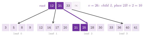
first item under its child \(j + 1\). In memory, the children of the node \(k\) of
a level are the nodes \(k ( B + 1 ) , \ldots , k ( B + 1 ) + B\) of the next
level, so that no pointer is stored, and the levels follow one another, the
leaves last (Figure 6.3). The level of the leaves has
\(s_{H-1} = \lceil n / B \rceil\) nodes and each level above
\(s_\ell = \lceil s_{\ell+1} / ( B + 1 ) \rceil\), up to the root; there are
thus
levels, and a search reads one line per level, against the \(\log_2 n - \log_2 B\) misses of the binary search (5 lines for a million keys of 32 bits, against 20 probes, of which the last 4 share a line).
In a node, the child to take is the count of the keys smaller than \(v\).
On the arithmetic keys under std::less, the count runs on the whole line
with no branch, the places past the last item holding the largest value of
the type (or \(+\infty\)). For the integers of 32 and 64 bits and the floating
types, countLess() of CountLess.h (in ADS::detail) makes it, with
ADS_WITH_HIGHWAY, a few comparisons of the vectors of Google Highway
inlined at the instructions given to the compiler (SimdInline.h), each
giving a mask whose lanes a count of the lanes sums; Highway compares the
unsigned integers itself where the processor has no unsigned comparison
(for words of \(w\) bits, \(x \mapsto x \oplus 2^{w-1}\) maps \([ 0 , 2^w )\)
onto the signed words in the same order, since it subtracts \(2^{w-1}\) from
each value). Without it, and on the other types, it is the loop of the comparisons,
which the compiler may vectorize or not, and on the other orders a scan of
the keys in use. Its companion greaterBits() gives the items larger than a
key as the bits of a word, which §6.9 uses
(Algorithm 6.9).
Algorithm 6.9. The layout and the search of
SPlusTree (Slotin 2022), and the
count with no branch in a node; the levels are numbered from the root, 0,
to the leaves, \(H - 1\).
A search is thus a loop of counts, one per level, and upperBound() counts
the keys not larger than \(v\) instead.
Besides the two bounds, the tree answers contains() by lowerBound(),
reads the item of a place by operator[], and gives size(), empty()
and its height(), i.e., \(H\).
Lemma 6.10. An SPlusTree on \(n \ge 1\)
items has the height \(H\) of (6.5) and fewer than \(( B + 1 ) ( n / B + H )\)
places of items, i.e., \(n\) for the leaves and fewer than \(n / B + ( B + 1 )
H\) more; it is built in \(O( n )\) time for a fixed \(B\), and a search reads one node per
level, i.e., \(H\) lines of cache when \(B \, \mathrm{sizeof}( T ) = 64\). Its
lowerBound( v ) returns \(\mathrm{lowerBound}( v )\).
Proof. With \(s = s_{H-1} = \lceil n / B \rceil\), the level at the distance \(d\) from the leaves has \(\lceil s / ( B + 1 )^d \rceil\) nodes, since \(\lceil \lceil x \rceil / ( B + 1 ) \rceil = \lceil x / ( B + 1 ) \rceil\), and the root is the first level with one node, at \(d = \lceil \log_{B+1} s \rceil\), which gives (6.5). Since \(\lceil x \rceil < x + 1\), the nodes are fewer than \(\sum_{d = 0}^{H - 1} ( s / ( B + 1 )^d + 1 ) < s ( B + 1 ) / B + H\), and the places, \(B\) per node, fewer than \(( B + 1 ) s + B H \le ( B + 1 ) ( n / B + H )\), since \(s < n / B + 1\). The leaves, a copy of the items, are written once. A key of a node at the distance \(d \ge 1\) from the leaves is found by \(d - 1\) multiplications, while the keys at the distance \(d\) are at most \(B \lceil s / ( B + 1 )^d \rceil\); the construction thus costs \(O( n + B \sum_{d \ge 1} d ( s / ( B + 1 )^d + 1 ) )\), i.e., \(O( n + B H^2 )\), since \(\sum_{d \ge 1} d x^d = x / ( 1 - x )^2\) for \(x < 1\), which is \(O( n )\) for a fixed \(B\). The nodes start at multiples of \(B\) items in a vector aligned to 64 bytes. As for the search, the key \(j\) of a node is the first item under its child \(j + 1\). Hence the count of the keys smaller than \(v\) is the child that holds \(\mathrm{lowerBound}( v )\) (the places past the last item counting as \(+\infty\)), and in the leaf the count gives the place itself. \(\square\)
Its space is on huge pages when it reaches 2 MB (cf. §5.9), and a search therefore misses the TLB at most once. In two points the S+ tree differs from the B-tree layout of Khuong and Morin 2017: the leaves are the sorted array, the inner keys only routing the search, and a node is searched by a count instead of a search. The layout of Eytzinger (a heap order of the items) also reads one line for the last 4 levels of the binary search, and with the prefetch of the 16 descendants 4 levels down it hides the latency of the misses instead of avoiding them, at the price of the bandwidth. Khuong and Morin 2017 found it the fastest of the layouts of the binary search, and the B-tree layout, with a node per line, faster on the arrays that do not fit in the cache. B-trees with no pointers go back to the CSS trees of Rao and Ross 1999. Later, the FAST trees of Kim et al. 2010 laid out a binary tree in blocks of lines and pages and searched a block with SIMD comparisons. In a lookup among the classic, the compressed and the learned indexes of integers, the comparative study of Bellomo et al. 2025 finds the B-trees with SIMD searches the fastest.
In ADS/search/StaticSearch.h, the declarations of the functions and of
SPlusTree that a user calls are
// declarations of <ADS/search/StaticSearch.h>
template< class T , class C = std::less<> >
std::size_t branchlessLowerBound( const std::vector< T > & A , const T & v ,
                                  C less = C() );
template< class T , class Less = std::less< T > , std::size_t Bytes = 64 >
 requires std::is_trivially_copyable_v< T >
class SPlusTree
{
 public:
 using Item = T;
 static constexpr std::size_t B =
   sizeof( T ) <= Bytes ? std::max< std::size_t >( Bytes / sizeof( T ) , 2 )
                        : 2;
 SPlusTree( void );
 explicit SPlusTree( const std::vector< T > & A , Less less = Less() );
 std::size_t lowerBound( const T & v ) const;
 std::size_t upperBound( const T & v ) const;
 bool contains( const T & v ) const;
 const T & operator[]( std::size_t i ) const;
 std::size_t size( void ) const;
 bool empty( void ) const;
 int height( void ) const;
 };
6.4 The PGM-index¶
The PGM-index of Ferragina and Vinciguerra
2020 (PGMIndex< K , E , R >, on fewer
than \(2^{32}\) arithmetic keys) replaces the inner nodes of a B+-tree by a
model of the keys. Its items \(A[ 0 .. n )\) are the points \(( A[ i ] , i )\) of
the plane, a repeated key standing for its first place. An
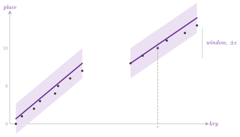
\(\epsilon\)-approximation is a sequence of segments, each a line
\(f( x ) = a + b ( x - k_s )\) over a range of keys from its first key \(k_s\),
such that \(| f( A[ i ] ) - i | \le \epsilon\) for each key of its range
(Figure 6.4). In turn, the first keys of the segments
are approximated, with error \(\epsilon_r\), by the segments of a level above,
and so on up to a single segment. By default, \(\epsilon = 64\) and
\(\epsilon_r = 4\).
The fewest segments, i.e., the optimal approximation, are found in one pass by the algorithm of O'Rourke 1981 as engineered by Xie et al. 2014 (Algorithm 6.10). Indeed, the lines that pass within \(\epsilon\) of the points of a range are those between the line of least slope and the line of largest slope that the convex hulls of the points moved up and down by \(\epsilon\) admit. A new point updates the two hulls in amortized \(O( 1 )\) time (Xie et al. 2014), and a range ends when a point leaves no line. A segment keeps the line of the average of the two extreme slopes through the point where they cross, and its slope is made not negative, so that the prediction never decreases; this line is within the error (Lemma 6.11). To make all this exact, the keys are first mapped to integers of 64 bits in the same order (the signed ones by flipping the top bit, the floating ones by their bits), and the hulls are kept with products of 128 bits.
Algorithm 6.10. The construction and the
search of PGMIndex (the optimal approximation of O'Rourke
1981 and Xie et al.
2014, and the search of Ferragina and
Vinciguerra 2020).
Lemma 6.11. Each segment of the optimal \(\epsilon\)-approximation but the last covers keys whose first places span at least \(2 \epsilon + 1\) places of \(A\) (at least \(2 \epsilon + 1\) keys when the keys are distinct); hence the last level has \(m \le \lceil n / ( 2 \epsilon + 1 ) \rceil\) segments, and there are at most \(1 + \lceil \log_{2 \epsilon_r + 1} m \rceil\) levels. On distinct keys a search costs
time, in a space of 28 bytes per segment besides the items. The line that a segment keeps, of the slope \(\max\{ ( \alpha^- + \alpha^+ ) / 2 , 0 \}\) through the crossing of the two extreme lines of slopes \(\alpha^- \le \alpha^+\), is within \(\epsilon\) of the points of its segment, in exact arithmetic.
Proof. We first show that the line kept is within the error. At each
abscissa \(x\), a line through the crossing \(P\) of the two extreme lines with
a slope between theirs takes a value between their values, on either side
of \(P\); both extreme lines take values in \([ y - \epsilon , y + \epsilon ]\)
at each point \(( x , y )\) of the segment, and so does such a line. The slope 0 is feasible too. If a line \(f\) of slope \(a < 0\) is within the error, then the horizontal line at the height \(f( x_k )\), with \(x_k\) the last
abscissa, is within it as well, since \(y_i - \epsilon \le y_k - \epsilon
\le f( x_k ) \le f( x_i ) \le y_i + \epsilon\), the places \(y_i\) not
decreasing; the feasible slopes are an interval, and \(\alpha^+ \ge 0\).
Hence \(\max\{ ( \alpha^- + \alpha^+ ) / 2 , 0 \}\) lies in \([ \alpha^- ,
\alpha^+ ]\). Then we show that the greedy, which closes a segment only when
no line is left, is optimal. If the points of a range are within
\(\epsilon\) of a line, so are those of any of its suffixes; hence, by
induction on \(j\), the \(j\)-th segment of the greedy ends no earlier than the
\(j\)-th segment of any other approximation, since it starts no later, and
the greedy uses the fewest segments. Now let a segment start at a point of
first place \(y\). Each later point whose first place is at most
\(y + 2 \epsilon\) is within \(\epsilon\) of the horizontal line through
\(y + \epsilon\); the segment is thus not closed before a point of first
place larger than \(y + 2 \epsilon\), which gives the first claim and the
bound on \(m\). At a level above, the points are the first keys of the level
below with the places \(0 , 1 , 2 , \ldots\), which are distinct, and the
same argument with \(\epsilon_r\) divides the segments by at least
\(2 \epsilon_r + 1\) per level. As for the search, let
\(k_s \le v < k_{s+1}\) for two first keys of the level below. Since the line does not decrease, and it is within \(\epsilon_r\) of \(s\) at \(k_s\) and of \(s + 1\)
at \(k_{s+1}\); hence its prediction at \(v\), truncated to an integer \(p\),
satisfies \(p - \epsilon_r - 1 \le s \le p + \epsilon_r + 1\). Our code searches the \(\epsilon_r + 2\) places on each side of \(p\), one more for the
rounding of the line in double, by a binary search of \(O( \log \epsilon_r )\)
comparisons. At the last level, on distinct keys, the same argument puts the
answer within \(\epsilon + 1\) places of the prediction, in a window of
\(2 \epsilon + 5\) places. Finally, a segment keeps its first key (8 bytes),
the two doubles of its line (16) and its first place (4). \(\square\)
At the last level, the window has its lines of cache prefetched at once, so that their misses overlap, and is searched by a binary search with no branch. On repeated keys, whose places a line cannot all approximate, the answer may be out of the window, and the search then goes on past it by galloping, at a cost logarithmic in the distance. Since the items are a copy on huge pages, the window adds no miss of the TLB.
Like the S+ tree, the index answers contains(), operator[], size(),
empty() and height() (its levels), and also gives segments(), the
segments \(m\) of the last level, and bytes(), the space of the levels
without the items. Note that this space is proportional to \(m\), which on
regular keys is far smaller than \(n / ( 2 \epsilon )\): on keys in
arithmetic progression, one segment covers them all. This is the point of
a learned index, whose space depends on the regularity of the keys more
than on their number.
In ADS/search/PGMIndex.h, the declarations of PGMIndex that a user
calls are
// declarations of <ADS/search/PGMIndex.h>
template< class K , std::size_t E = 64 , std::size_t R = 4 >
 requires std::is_arithmetic_v< K >
class PGMIndex
{
 public:
 using Item = K;
 PGMIndex( void );
 explicit PGMIndex( const std::vector< K > & A );
 std::size_t lowerBound( const K & v ) const;
 bool contains( const K & v ) const;
 const K & operator[]( std::size_t i ) const;
 std::size_t size( void ) const;
 bool empty( void ) const;
 std::size_t segments( void ) const;
 int height( void ) const;
 std::size_t bytes( void ) const;
 };
6.5 The compressed PGM-index¶
The compressed PGM-index of Ferragina and Vinciguerra
2020 (CompressedPGMIndex< K , E >)
keeps the segments in a few tens of bits each instead of 28 bytes, with the
same search at the last level. Consider the lines that are within \(\epsilon\)
of the \(k\) points of a segment, i.e., the pairs \(( \alpha , \beta )\) with
\(| \beta + \alpha x_i - y_i | \le \epsilon\) for each of its points. They are
the intersection of \(2 k\) half-planes, a convex region, whose shadow on the
axis of the slopes is the interval \([ \alpha^- , \alpha^+ ]\) between the two
extreme lines of the algorithm of O'Rourke. Each slope of the interval has an
intercept within the error, the middle of
hence a set of slopes serves all the segments if it hits each of their intervals (Figure 6.5).
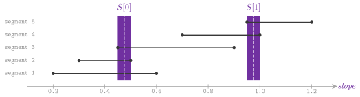
Lemma 6.12. Sort the intervals by their left ends, and grow a group while the next interval meets the intersection of the group, opening a new group otherwise. One slope per group, in its intersection, hits all the intervals, and no set of fewer slopes does.
Proof. Each interval of a group contains the intersection of the group, which is not empty by construction. In each group, let \(I_g\) be the interval of least right end, which is the right end of the intersection; the first interval of the next group begins after it, and so do all the later ones, since the left ends increase. The intervals \(I_g\) are thus pairwise disjoint, and a slope hits at most one of them; as many slopes as groups are therefore needed. \(\square\)
Each segment then keeps the index of its slope and its intercept by (6.7), as a distance from its first place of at most \(\epsilon + 1\) (at most \(\epsilon\) with the exact slope, one more for its rounding). The first places of the segments, increasing, are kept by Elias-Fano (cf. §22.6), and their first keys whole, searched by a separate PGM-index (with \(\epsilon = \epsilon_r = 4\)) in place of the levels above (Algorithm 6.11). With \(m\) segments and \(\sigma\) slopes, this takes
bits per segment, plus the segments of the PGM-index of the keys, the directory of Elias-Fano and the table of the slopes, \(32 \sigma\) bits in single precision (as in the implementation of the paper).
Algorithm 6.11. The construction and the
search of CompressedPGMIndex (Ferragina and Vinciguerra
2020); \(k_s\) and \(p_s\) are the first
key and the first place of the segment \(s\).
Elias-Fano on the first keys would save \(62 - \log_2( u / m )\) bits a
segment, for keys in a universe of size \(u\). Yet, its rank (the search of
a segment) scans the bucket of the key, and on skewed keys most of the
first keys crowd into a few buckets. In contrast, the PGM-index of the keys
finds the segment in the time of the levels of the plain PGM-index, and a
search adds to that two selects and a field of bits. However, the rounding of a
shared slope to a float may take a line out of the error; the
construction checks each segment, and gives its own slope (appended to the
table) to one whose line misses a point by more than \(\epsilon + 1\). Besides
lowerBound(), the class has the same accessors as PGMIndex but
height(), and gives the number of its slopes by slopes().
In ADS/search/CompressedPGMIndex.h, the declarations of
CompressedPGMIndex that a user calls are
// declarations of <ADS/search/CompressedPGMIndex.h>
template< class K , std::size_t E = 64 >
 requires std::is_arithmetic_v< K >
class CompressedPGMIndex
{
 public:
 using Item = K;
 CompressedPGMIndex( void );
 explicit CompressedPGMIndex( std::vector< K > A );
 std::size_t lowerBound( const K & v ) const;
 bool contains( const K & v ) const;
 const K & operator[]( std::size_t i ) const;
 std::size_t size( void ) const;
 bool empty( void ) const;
 std::size_t segments( void ) const;
 std::size_t slopes( void ) const;
 std::size_t bytes( void ) const;
 };
6.6 The dynamic PGM-index¶
The dynamic PGM-index (DynamicPGMIndex< K , V , E , B , I >) is an ordered
map from arithmetic keys to values, with insertions and removals, made of
static PGM-indexes by the logarithmic method of Bentley and Saxe
1980. The pairs lie in a sorted buffer
\(L_0\) of \(b_0 = 128\) pairs (kBuffer) and in sorted levels
\(L_1 , L_2 , \ldots\) of capacities \(c_t = b_0 B^t\) (\(B = 8\) by default), each
key at most once per level. A key may be in several levels, and its pair in
the newest one (the buffer first, then by increasing \(t\)) is the one that
counts; a removal (erase()) inserts a tombstone, a pair that marks the key
as absent. When an insertion finds the buffer full, the buffer is merged, with
the new pair and with the levels before \(L_t\), into the first level \(L_t\) that
has room for them all (Algorithm 6.12 and Figure
6.6). A constructor puts a vector of pairs, sorted by
distinct keys, into the one level that holds them.

Algorithm 6.12. The operations of
DynamicPGMIndex (the logarithmic method of Bentley and Saxe
1980); \(\| L \|\) is the number of the
pairs of a level and \(c_i = b_0 B^i\) the capacity of \(L_i\).
Lemma 6.13. An insertion or a removal costs \(O( B \log_B( n / b_0 ) )\) amortized time, \(n\) the pairs inserted, and a lookup searches \(O( \log_B( n / b_0 ) )\) levels; the filters of the levels add \(O( 1 )\) amortized insertions into a filter per pair and level.
Proof. \(L_t\) is chosen because the pairs of the buffer and of the levels before \(L_{t-1}\) do not fit in the room left in \(L_{t-1}\); with those of \(L_{t-1}\), they are thus more than \(c_{t-1} = c_t / B\) (more than \(b_0\) for \(t = 1\), since the buffer holds \(b_0 + 1\) pairs with the new one). Merging and building the PGM-index of the result are linear, \(O( c_t )\), i.e., \(O( B )\) per pair brought into \(L_t\). A pair is brought into a level only from the levels before it, hence into each level at most once. Finally, a level \(L_t\) is created only when more than \(c_{t-1}\) pairs exist, and therefore \(t < 1 + \log_B( n / b_0 )\). A filter receives each pair that a merge brings into its level once. It is built again, for twice the keys, only when it is full, i.e., after as many insertions as the keys it held, and the insertions of a rebuilding are thus paid by those that filled it. \(\square\)
A lookup (find(), which gives a pointer to the value, nil if the key is
absent, valid until the next change, and contains()) stops at the newest
level that has the key. In turn, lowerBound() and the visit of a range
(forEach()) merge the levels from their places of the key, and skip the
keys whose newest pair is a tombstone. Tombstones are dropped when the
merge lands on the last level, where no older pair is left for them to
hide. Several choices of the layout fix the constants. As in the
implementation of the paper, only the levels of capacity at least \(I\)
(kIndexed, \(2^{24}\) by default) have a PGM-index, with \(\epsilon = E\)
(16 by default) and \(\epsilon_r = 4\), since on the smaller ones a model
does not pay for its construction at each merge; the others are searched by
the binary search with no branch of §6.3. The keys
and the values of a level are two arrays, so that a search reads only the
keys, and the tombstones are a sorted list of their keys apart (they are
usually few). A level of capacity at least \(2^{12}\) (kFiltered) also has
a blocked filter of Bloom of its keys (cf. §10.8),
10 bits per key, as the levels of the stores by log-structured merge have
(O'Neil et al. 1996; Dayan et al.
2017). A lookup of a key that is not
there thus reads one line of cache per level instead of searching each,
and one that is there reads a line per newer level and searches only its
(false positives aside). The filter of a level takes the keys that a merge
brings in, and is built again, for twice the keys, only when it is full;
the filters thus add a constant number of insertions into a filter per key
and level to the cost (cf. Lemma 6.13). We do not keep the number of the distinct keys, since it would cost a lookup per insertion.
Instead, entries() counts the pairs stored, tombstones and older pairs included,
and levels() the levels below the buffer, empty or not.
In ADS/search/DynamicPGMIndex.h, the declarations of DynamicPGMIndex
that a user calls are
// declarations of <ADS/search/DynamicPGMIndex.h>
template< class K , class V , std::size_t E = 16 , std::size_t B = 8 ,
          std::size_t I = ( std::size_t( 1 ) << 24 ) >
 requires std::is_arithmetic_v< K >
class DynamicPGMIndex
{
 public:
 using key_type = K;
 using mapped_type = V;
 static constexpr std::size_t kBuffer = 128;
 static constexpr std::size_t kIndexed = I;
 static constexpr std::size_t kFiltered = std::size_t( 1 ) << 12;
 DynamicPGMIndex( void );
 explicit DynamicPGMIndex( const std::vector< std::pair< K , V > > & P );
 void insert( const K & k , const V & v );
 void erase( const K & k );
 const V * find( const K & k ) const;
 bool contains( const K & k ) const;
 std::optional< std::pair< K , V > > lowerBound( const K & k ) const;
 template< class F >
 void forEach( const K & lo , const K & hi , F && f ) const;
 std::size_t entries( void ) const;
 std::size_t levels( void ) const;
 };
6.7 The minimum and the local optima¶
min() of Minimum.h keeps the minimum so far and compares it with each
of the other items, and argmin() gives the place of the first minimum of
a range, as the selection sort of Montresor 2025,
§2.7.1 needs
(Algorithm 6.13).
Lemma 6.14. Each comparison-based algorithm
that finds the minimum of \(n\) distinct items makes at least \(n - 1\)
comparisons (Montresor 2025, §2.6),
and min() makes \(n - 1\). The minimum and the maximum together need
comparisons, which minMax() makes (Pohl
1972).
Proof. An item that has never lost a comparison may still be the
minimum, and a comparison makes at most one item lose for the first time;
hence \(n - 1\) comparisons are needed to leave a single item that never
lost. For the minimum and the maximum, each item but one must lose once,
and each item but one must win once; we call these \(2 n - 2\) first losses
and first wins the units of information. An adversary keeps a value for
each item and answers by it, with the freedom to raise an item that never
lost and to lower an item that never won, which leaves all the past
answers true. When an item that never lost meets one that has lost, the
former wins (raised if needed); when two items that have both lost (or
both never lost, at most one of them new) meet, it answers so that at most one of
them gets its first win (lowering one that never won) or its first loss
(raising one that never lost). Each comparison thus gives at most one unit,
except a comparison of two items never compared, which gives two. There are
at most \(\lfloor n / 2 \rfloor\) such comparisons, and hence at least
\(\lfloor n / 2 \rfloor + ( 2 n - 2 - 2 \lfloor n / 2 \rfloor ) =
\lceil 3 n / 2 \rceil - 2\) comparisons. minMax() pairs the items, compares
the two of a pair, and then the smaller with the minimum and the larger with
the maximum, 3 comparisons per pair, after 1 for the first pair when \(n\) is
even, which gives (6.9) for \(n\) even and odd. \(\square\)
Algorithm 6.13. The minimum (Montresor 2025, §1.2 and §2.7.1), and the minimum and the maximum together by pairs and by halves (Pohl 1972).
Lemma 6.15. minMaxDivide() makes \(T( n
)\) comparisons, with \(T( 1 ) = 0\), \(T( 2 ) = 1\) and \(T( n ) = T( \lceil n
/ 2 \rceil ) + T( \lfloor n / 2 \rfloor ) + 2\) for \(n \ge 3\); hence \(T( n
) = 3 n / 2 - 2\), i.e., (6.9), when \(n\) is a power of 2.
Proof. A part of one item costs nothing, one of two items one comparison, and a longer one is split at its middle into parts of \(\lceil n / 2 \rceil\) and \(\lfloor n / 2 \rfloor\) items, whose minima and maxima are then compared, two comparisons. For \(n = 2^k\), \(k \ge 1\), by induction \(T( 2^k ) = 2 ( 3 \cdot 2^{k-2} - 2 ) + 2 = 3 \cdot 2^{k-1} - 2\), and \(T( 2 ) = 1\) is the case \(k = 1\). \(\square\)
On other lengths it may make a few more (8 instead of 7 for \(n = 6\)).
A local optimum is cheaper than the minimum. A peak of \(A\) is an item
not smaller than its neighbours, the places out of \(A\) counting as
\(-\infty\); one always exists (e.g., the maximum). findPeak() of
LocalOptima.h keeps the invariant that \(A[ \mathit{lo} .. \mathit{hi} ]\)
holds a peak of \(A\), which is true when \(A[ \mathit{lo} - 1 ] < A[ \mathit{lo} ]\)
(or \(\mathit{lo} = 0\)) and \(A[ \mathit{hi} ] \ge A[ \mathit{hi} + 1 ]\) (or
\(\mathit{hi} = n - 1\)). Indeed, under these conditions the maximum of the
part is a peak of \(A\): inside the part its neighbours are not larger, and
at an end the neighbour out of the part is smaller or not larger by the
conditions (Algorithm 6.14).
Lemma 6.16. findPeak() returns a peak of
\(A\) after at most \(\lceil \log_2 n \rceil\) comparisons. On a binary tree
of height \(h\), localMinimum() returns a node smaller than its parent (or
the root) and not larger than its children, after at most \(2 ( h + 1 )\)
comparisons.
Proof. Comparing \(A[ m ]\) with \(A[ m + 1 ]\) keeps the invariant on one of the two halves: if \(A[ m ] < A[ m + 1 ]\), the part \(A[ m + 1 .. \mathit{hi} ]\) rises into \(m + 1\); otherwise the part \(A[ \mathit{lo} .. m ]\) falls out of \(m\). A part of \(\ell\) items leaves at most \(\lceil \ell / 2 \rceil\), and a part of one item is a peak by the invariant; Lemma 1.5 gives the bound. The walk on the tree moves from a node to a child smaller than it, so that the node where it stops, at a depth at most \(h\), is smaller than its parent (or is the root), and it stops because no child is smaller; each node of the path costs at most two comparisons. \(\square\)
Algorithm 6.14. A peak and a local minimum of a vector, and a local minimum of a binary tree (Esercizi Divide-et-impera and Esercizi Alberi of Montresor 2025).
A peak thus costs \(\lceil \log_2 n \rceil\) comparisons, against the
\(n - 1\) of the maximum; localMinimum() of a vector is the same search
with the order reversed, and on a binary tree the walk takes the left
child first. On general graphs, however, no such bound exists, since a local minimum on the hypercube of dimension \(d\) needs
about \(2^{d / 2}\) evaluations, even for a randomized algorithm (Aldous
1983).
In ADS/search/Minimum.h, the functions are declared as
// declarations of <ADS/search/Minimum.h>
template< class T , class C = std::less<> >
std::size_t argmin( const std::vector< T > & A , std::size_t start ,
                    std::size_t end , C less = C() );
template< class T , class C = std::less<> >
const T & min( const std::vector< T > & A , C less = C() );
template< class T , class C = std::less<> >
std::pair< T , T > minMax( const std::vector< T > & A , C less = C() );
template< class T , class C = std::less<> >
std::pair< T , T > minMaxDivide( const std::vector< T > & A , C less = C() );
In ADS/search/LocalOptima.h, the functions are declared as
// declarations of <ADS/search/LocalOptima.h>
template< class T , class C = std::less<> >
std::size_t findPeak( const std::vector< T > & A , C less = C() );
template< class T , class C = std::less<> >
std::size_t localMinimum( const std::vector< T > & A , C less = C() );
template< class T , class C = std::less<> >
BinaryTree< T > * localMinimum( BinaryTree< T > * t , C less = C() );
6.8 The selection¶
The item of rank \(k\) can be found without sorting. The selection of Hoare
1961 (selection() of Selection.h,
Montresor 2025, §17.1) partitions
the part around a pivot as quicksort does, and goes on only in the side
that holds the rank \(k\) (Algorithm 6.15). The
pivot is chosen at random when a generator is given, and is the first
item of the part otherwise. With a random pivot its rank is uniform, the
side kept is in the worst case the larger one, and the expected number of
comparisons satisfies (6.10) below.
Lemma 6.17. Let \(T( n )\) be the largest,
over the ranks \(k\) and the orders of \(n\) distinct items, of the expected
number of comparisons of selection() with a random pivot. Then
and \(T( n ) \le 4 n\); with the first item as the pivot, an increasing vector and \(k = n\) cost \(n ( n - 1 ) / 2\) comparisons.
Proof. A partition of a part of \(n\) items compares the pivot with the other \(n - 1\), and the pivot has the rank \(q\) with probability \(1 / n\), each \(q\) in \(1 , \ldots , n\). The part kept has \(q - 1\) or \(n - q\) items, at most \(\max\{ q - 1 , n - q \}\), and each value \(q' \ge \lfloor n / 2 \rfloor\) of this maximum comes from at most two values of \(q\). With \(T\) taken not decreasing (it is a maximum over the ranks, and a longer part can hold a shorter one), (6.10) follows. One has \(\sum_{q = \lfloor n / 2 \rfloor}^{n - 1} q \le 3 n^2 / 8\) (it is \(3 n^2 / 8 - n / 4\) for \(n\) even and \(3 ( n^2 - 1 ) / 8\) for \(n\) odd); hence, by induction with \(T( q ) \le 4 q\), \(T( n ) \le n - 1 + ( 2 / n ) \cdot 4 \cdot 3 n^2 / 8 = n - 1 + 3 n \le 4 n\). With the first item of an increasing part as the pivot, the part loses one item per round, and the rounds cost \(( n - 1 ) + ( n - 2 ) + \cdots + 1\). \(\square\)
The selection is thus linear in expectation on every input, while a pivot that is always the smallest item gives \(\Theta( n^2 )\).
Algorithm 6.15. The selection of Hoare 1961 (Montresor 2025, §17.1) and the median of the medians (Blum et al. 1973).
Lemma 6.18. If the pivot is the median of the medians of the groups of 5 items, at least \(3 n / 10 - O( 1 )\) items lie on each side of it, and the selection makes
comparisons in the worst case (Blum et al. 1973).
Proof. There are \(M = \lfloor n / 5 \rfloor \ge ( n - 4 ) / 5\) groups, and the pivot is the median of rank \(\lceil M / 2 \rceil\) of their medians. At least \(\lceil M / 2 \rceil\) medians are not larger than the pivot, each with 3 items of its group not larger than it, and the same holds on the other side; hence each of the parts smaller and larger than the pivot has at most \(n - 3 ( n - 4 ) / 10 \le 7 n / 10 + 2\) items. Each group costs at most 10 comparisons of insertion each, and the partition in three ways at most 2 per item, so that, with \(T\) taken not decreasing, \(T( n ) \le T( n / 5 ) + T( 7 n / 10 + 2 ) + a n\) for \(n > 10\) and a constant \(a\). For \(n \ge 80\) one has \(7 n / 10 + 2 \le 3 n / 4\), and by induction \(T( n ) \le c n\) with \(c = \max\{ 20 a , \max_{n < 80} T( n ) / n \}\), since \(c n / 5 + 3 c n / 4 + a n = 19 c n / 20 + a n \le c n\). \(\square\)
medianOfMedians() partitions in three ways (smaller, equal and larger
than the pivot), so that many equal items cost no further round, and
sorts the parts of at most 10 items by insertion. Both functions take the
rank from 1 and rearrange \(A\).
The engineered nthElement() of NthElement.h puts in the place nth
of a range the item that would be there if the range were sorted, the
items before it not larger and those after it not smaller, as
std::nth_element, which it is meant to replace; an overload on a vector
takes the rank \(k\) from 0 and returns the item
(Algorithm 6.16). On a range of \(n > 600\) items,
the pivot comes from the sampling of Floyd and Rivest
1975: a sample of about
\(s = n^{2/3} / 2\) items around the place \(k\) is selected recursively for
the rank \(k\), and the item that lands in the place \(k\) then falls, with
high probability, just on the side of \(k\) that leaves the smaller part.
The expected number of comparisons is
(Kiwiel 2005), which is optimal up to the last term, against the \(2 n + 2 k \ln( n / k ) + 2 ( n - k ) \ln( n / ( n - k ) ) + o( n )\) of a pivot at random (up to \(2 ( 1 + \ln 2 ) n \approx 3.39 n\) for the median). Below 600 items the pivot is the median of three, and a range of at most 24 items is sorted by insertion.
Algorithm 6.16. The engineered selection
(the selection of Hoare 1961 with the
sample of Floyd and Rivest 1975), and
its partition of Lomuto with no branch; the range is \(A[ 0 .. n - 1 ]\) and
\(k\) the place nth.
The partition suits the order of the range, which 64 items taken at a stride reveal. On a random order (more than 16 turns, i.e., a rise followed by a fall or the opposite, among them; about \(2 \cdot 62 / 3 \approx 41\) on a random permutation) it is the scheme of Lomuto with no branch. An item is moved to the end of the smaller ones and the item there to its place, and the end advances by the outcome of the comparison, an addition instead of a jump (Edelkamp and Weiß 2016 apply the same idea to quicksort), while the partition of Hoare mispredicts half of its comparisons on random items. We unroll the loop by 4, so that it does not depend on the alignment of one jump.
Lemma 6.19. selectLomuto() makes \(n -
1\) comparisons and returns a place \(q\) such that \(A[ q ] = p\), the items
before \(q\) are smaller than \(p\) (not larger, when the equal items go
left), and those after \(q\) are not.
Proof. Call an item left when the test of line 5 holds for it. We show that after the iteration \(i\) of line 3 the items of \(A[ 1 .. \ell - 1 ]\) are left and those of \(A[ \ell .. i ]\) are not, with \(1 \le \ell \le i + 1\); this holds before the first iteration, with \(\ell = 1\) and an empty second range. Line 4 exchanges \(x = A[ i ]\) with \(A[ \ell ]\), which is an item that is not left when \(\ell < i\), and \(x\) itself when \(\ell = i\). If \(x\) is left, line 5 extends the first range by the place \(\ell\) that now holds \(x\), and the item moved to the place \(i\) is not left; if \(x\) is not left, it stays at the place \(\ell\), the first of the second range. After the last iteration, \(A[ 1 .. \ell - 1 ]\) are left and \(A[ \ell .. n - 1 ]\) are not; line 6 moves \(p\) to the place \(q = \ell - 1\) and the left item there, if \(q > 0\), to the place 0. Each iteration makes one comparison, and there are \(n - 1\) of them. \(\square\)
On a range in some order (an organ pipe, a few runs) the partition is the scheme of Hoare, whose branches are then predicted and which writes only the items on the wrong side; the sample of Floyd and Rivest is then gathered from the whole range at a stride, since a contiguous one would not represent it. A range whose 64 items all rise (or all fall) is checked to be sorted, by blocks of 64 pairs with no exit inside a block, and is then left as it is (or reversed in the same pass of the check), in about \(n\) comparisons. When the pivot is the smallest item of the range, the items equal to it go to its left, so that many equal items end in one step; since the items of a range cut on its left by a pivot are not smaller than it, a later pivot equal to it is known to be the smallest with no pass. Finally, each round charges the items of its part to a budget of \(4 n\) items, which a random order hardly ever exhausts (by (6.12), the rounds of a random range of more than 600 items partition about \(1.5 n\) items at most). A round whose part the rest of the budget does not cover takes as its pivot the median of the medians, as the selection of Musser 1997 does by the same device. When the part such a round leaves on the right of its pivot holds more than \(7 m / 10 + 2\) of its \(m\) items, which on distinct items never happens, a second partition of that part puts the items equal to the pivot on its left as well; the part kept then holds the larger items only.
Lemma 6.20. On \(n\) items, distinct or
not, nthElement() takes \(O( n )\) time in the worst case.
Proof. Let \(S( n )\) be the worst-case time of select() on a part of \(n\)
items, which has its own budget of \(4 n\). In a call, the rounds act on
nested parts, each smaller than the one before, since the pivot is left
out; there are therefore at most \(n\) of them, and those charged to the
budget partition at most \(4 n\) items in all. A round with \(m > 600\)
selects recursively a sample of \(\mathit{hi} - \mathit{lo} + 1 \le s + | d
| + 2\) items, with \(s = m^{2/3} / 2\) and \(| d | \le \sqrt{s \ln m} / 2\);
the three ratios to \(m\) decrease for \(m \ge 601\), and there they sum to
less than \(0.0592 + 0.0126 + 0.0034 < 0.076\), so that the samples hold
fewer than \(0.076 \cdot 4 n < 0.31 n\) items in all.
Let \(m_1 > m_2 > \cdots > m_J\) (all above 24) be the parts of the rounds of the median of the medians. Such a round on \(m\) items sorts \(g = \lfloor m / 5 \rfloor \ge ( m - 4 ) / 5\) disjoint groups of 5 (the exchange that moves the median of a group to the front touches only places of the groups already sorted), and its pivot \(p\) is the item of rank \(\lfloor g / 2 \rfloor\), from 0, of their medians. Hence \(\lfloor g / 2 \rfloor + 1\) medians are not larger than \(p\) and \(\lceil g / 2 \rceil\) are not smaller, each with two more items of its group on the same side, so that at least \(3 ( \lfloor g / 2 \rfloor + 1 ) \ge 3 ( m + 1 ) / 10\) items are not larger than \(p\) and at least \(3 \lceil g / 2 \rceil \ge 3 ( m - 4 ) / 10\) are not smaller. The part kept is one of three: the items smaller than \(p\), at most \(m - 3 ( m - 4 ) / 10 = 7 m / 10 + 6 / 5\); the items after \(p\) when the first partition puts them on the right, kept only if they are at most \(7 m / 10 + 2\); or the items larger than \(p\) (after the second partition, or when the items equal to \(p\) go left at once), at most \(m - 3 ( m + 1 ) / 10 < 7 m / 10\). Therefore \(m_{j+1} \le 7 m_j / 10 + 2\), i.e., \(m_{j+1} - 20 / 3 \le 0.7 ( m_j - 20 / 3 )\), whence \(m_j - 20 / 3 \le 0.7^{j-1} n\); since \(m_j > 24\), this gives \(J \le 1 + \log_{10/7}( n / 17 )\), and \(\sum_j m_j \le n / 0.3 + 20 J / 3\), so that the medians hold at most \(\sum_j \lfloor m_j / 5 \rfloor \le n / 1.5 + 4 J / 3 < 0.67 n + 4 J / 3\) items in all.
Besides the recursive calls, a call spends \(O( 1 )\) per round and \(O( m )\)
per partition (at most two), per sort of the groups and per test of an
order in a round on \(m\) items; by the two sums above, this is at most \(a n\)
for a constant \(a\). The recursive calls are on fewer than \(0.31 n + 0.67 n
+ 4 J / 3 < 0.98 n\) items in all for \(n \ge n_0\), since \(J = O( \log n )\).
By induction, therefore, \(S( n ) \le a n + 0.98 c n \le c n\) for \(n \ge
n_0\) and \(c \ge 50 a\), with \(c\) large enough for \(n < n_0\) as well. The
scan of nthElement() for a range in order adds \(O( n )\). \(\square\)
On distinct items the part on the right of a pivot of the median of the
medians never exceeds \(7 m / 10\), so that the second partition never runs
and the comparisons are, one by one, those of the selection without it.
Without it, on the other hand, a first partition that leaves on the right
all the items equal to the pivot may keep almost the whole part, and the
argument above would fail. Against the adversary of McIlroy
1999, which fixes the order of the
items while they are compared, the comparisons stay below \(16 n\) from \(n
= 2^{12}\) to \(2^{18}\), where a budget counted in rounds let them grow with
\(\log n\), and they stay there when the adversary gives each value to 2, 10
or 100 items (the test ordered.nth-element-adversary).
Table 6.2 compares the three selections.
Table 6.2. The selections of the item of
rank \(k\) in ADS/search.
| Function | Pivot | Comparisons |
|---|---|---|
selection() |
at random, or the first item | \(O( n )\) expected by (6.10), \(\Theta( n^2 )\) in the worst case |
medianOfMedians() |
the median of the medians of the groups of 5 | \(O( n )\) in the worst case, by (6.11) |
nthElement() |
the sample of Floyd and Rivest, the median of three on short parts | (6.12) expected, \(O( n )\) in the worst case |
In ADS/search/Selection.h, the functions are declared as
// declarations of <ADS/search/Selection.h>
template< class T , class R = std::mt19937 >
T selection( std::vector< T > & A , std::size_t k , R * rng = nullptr );
template< class T >
T medianOfMedians( std::vector< T > & A , std::size_t k );
In ADS/search/NthElement.h, the functions are declared as
// declarations of <ADS/search/NthElement.h>
template< std::random_access_iterator It , class C = std::less<> >
void nthElement( It first , It nth , It last , C less = C() );
template< class T , class C = std::less<> >
T nthElement( std::vector< T > & A , std::size_t k , C less = C() );
6.9 Range minima¶
After a preprocessing of \(A\), the query \(\mathrm{RMQ}( i , j )\) is
answered without scanning the range; the problem underlies the longest
common extensions of a text and the lowest common ancestors of a tree
(cf. §15.5 and §8.4). The
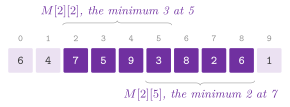
sparse table (SparseTable of RangeMinimum.h) stores
\(M[ L ][ i ] = \mathrm{RMQ}( i , i + 2^L - 1 )\) for each \(i\) and \(L\), each
from two entries of the row before. A query takes the better of the two
entries of length \(2^L\), \(L = \lfloor \log_2 ( j - i + 1 ) \rfloor\), that
start at \(i\) and end at \(j\) (Algorithm 6.17 and
Figure 6.7).
Algorithm 6.17. The sparse table (Bender and Farach-Colton 2000); the better of two places is the one of the smaller item, the left one on a tie.
Lemma 6.21. The sparse table of \(n\) items is built in \(O( n \log n )\) time and space, and its query returns \(\mathrm{RMQ}( i , j )\) in \(O( 1 )\) time.
Proof. The range of length \(2^{L+1}\) from \(i\) is the union of the ranges of length \(2^L\) from \(i\) and from \(i + 2^L\), and the leftmost minimum of a union of two ranges, the first before the second, is the better of their leftmost minima, the left one on a tie; by induction on \(L\), each entry is right. There are \(\lfloor \log_2 n \rfloor + 1\) rows of at most \(n\) entries, each computed in \(O( 1 )\) time. For a query, \(2^L \le j - i + 1 < 2^{L+1}\), so that the ranges \([ i , i + 2^L - 1 ]\) and \([ j - 2^L + 1 , j ]\) lie in \([ i , j ]\) and cover it. The leftmost minimum of \([ i , j ]\) is in one of them, and the better of their two answers, the left one on a tie, is it, since an item of the overlap that is a minimum is reached first from the left range. \(L\) is the position of the leading bit of \(j - i + 1\), one instruction. \(\square\)
The linear preprocessing rests on a tree. The Cartesian tree of \(A\)
(Vuillemin 1980) has the leftmost
minimum of \(A\) as its root, and the Cartesian trees of the parts on its
left and on its right as its subtrees. cartesianTree() builds it, as the
parent of each place (\(n\) for the root), with a stack that holds its right
spine (Algorithm 6.18). Equal items go to the
right.
Algorithm 6.18. The Cartesian tree of \(A\) (Vuillemin 1980), the stack \(S\) holding the right spine of the tree of \(A[ 0 .. i - 1 ]\).
Lemma 6.22. cartesianTree() returns the
parents of the Cartesian tree of \(A\), in which an item equal to an
ancestor lies in its right subtree, in \(O( n )\) time and space.
Proof. We show by induction on \(i\) that after the step \(i\) the parents computed for \(A[ 0 .. i ]\) are those of the Cartesian tree of \(A[ 0 .. i ]\), and \(S\) holds its right spine, i.e., the path from the root along the right children, from the bottom up. Being the last of the invisit, the new item \(A[ i ]\) is on the right spine, and its ancestors are the items of the old spine not larger than it (the minimum of a range that ends at \(i\), the leftmost on ties, is the first item of the spine from the root that is not larger than \(A[ i ]\), or \(A[ i ]\) itself). Our step pops the items of the spine larger than \(A[ i ]\), which become its left subtree (the last popped is its left child), and makes \(A[ i ]\) the right child of the new top, or the root if the stack is empty; this is the tree of \(A[ 0 .. i ]\). Each place is pushed once and popped at most once. \(\square\)
Lemma 6.23. \(\mathrm{RMQ}( i , j )\) is the lowest common ancestor of \(i\) and \(j\) in the Cartesian tree of \(A\), i.e., the node of least depth among those that the Euler tour of the tree visits between the first visits of \(i\) and \(j\) (Bender and Farach-Colton 2000).
Proof. The invisit of the tree is \(A\), and each subtree is thus a range of places. Going down from the root, while the place of the node is out of \([ i , j ]\) both \(i\) and \(j\) lie in the same subtree; the lowest common ancestor \(a\) is therefore the first node of the path whose place falls in \([ i , j ]\), and the range lies in the range of the subtree of \(a\). The root \(a\) of that subtree is the leftmost minimum of its range, and hence of \([ i , j ]\): an item equal to it on its left is an ancestor of \(a\), since equal items go to the right, hence out of its subtree. Between the two first visits the tour does not leave the subtree of \(a\), and it visits \(a\) (at the start, if \(a\) is \(i\), or between the two subtrees of \(a\) otherwise), the only node of least depth there. \(\square\)
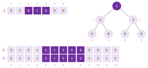
The depths along a tour differ by exactly 1 at each step, and the queries
on such an array (PlusMinusOneRangeMinimum) are answered in \(O( 1 )\)
time after \(O( n )\) preprocessing. The array is cut into blocks of
\(d = \max\{ 1 , \lfloor \lfloor \log_2 n \rfloor / 2 \rfloor \}\) items
(blockSize()), and a sparse table on the \(n / d\) minima of the blocks
costs \(O( ( n / d ) \log n ) = O( n )\). A block is determined, up to an
additive constant, by its \(d - 1\) steps of \(\pm 1\); hence the answers
inside all the possible blocks are built once in a table (the trick of the
Four Russians, Arlazarov et al. 1970)
of
entries (Algorithm 6.19). Then RangeMinimum
answers by the query on the \(2 n - 1\) depths of the tour of the Cartesian
tree of \(A\) (Figure 6.8), whose nodes eulerTour()
gives.
Algorithm 6.19. The range minima on steps of \(\pm 1\) and on any array (Bender and Farach-Colton 2000).
Lemma 6.24. PlusMinusOneRangeMinimum
answers a query in \(O( 1 )\) time after \(O( n )\) preprocessing, with the
table (6.13), and so does RangeMinimum on any array of \(n\) items.
Proof. With \(d \approx \log_2 n / 2\), the blocks are \(\lceil n / d \rceil\),
and the sparse table on their minima takes \(O( ( n / d ) \log n ) = O( n
)\) by Lemma 6.21. A block \(D[ b .. b + d - 1 ]\)
equals \(D[ b ]\) plus the prefix sums of its \(d - 1\) steps, so that its leftmost minima are those of the block of the same steps starting at 0. There are \(2^{d-1}\) such patterns, each with \(d^2\) answers, and \(2^{d-1}
d^2 \le 2^{\log_2 n / 2 - 1} ( \log_2 n / 2 )^2 \le \sqrt{n} \log_2^2 n\),
which the table holds after \(O( \sqrt{n} \log_2^2 n ) = o( n )\) time. A
query in one block reads the table, and one across blocks takes the better
of the suffix of the first block, of the prefix of the last and of the
sparse table on the blocks between, \(O( 1 )\) reads. For RangeMinimum, the Cartesian tree (Lemma 6.22) and its Euler tour, whose consecutive depths differ by 1, take \(O( n )\) time. By
Lemma 6.23 a query is a query on the depths
between the first visits of \(i\) and \(j\), mapped back to its node. \(\square\)
The bound \(O( n )\) was first reached by Harel and Tarjan
1984 on the lowest common ancestors,
with a far more involved structure; Fischer and Heun
2011 need only \(2 n + o( n )\) bits
besides \(A\), by describing each block by its Cartesian tree, which
removes the Euler tour and its factor 2. In practice the constant factors
of the reduction are large, and the sparse table, the simplest of the
three, is often faster on the arrays that fit in a cache. All the
structures of the section keep a copy of the array, which size() and
operator[] read (and SparseTable and RangeMinimum also as a range of
constant iterators); PlusMinusOneRangeMinimum gives only its size().
WordRangeMinimum keeps the decomposition into blocks but answers inside
a block of 64 items by the bits of a word. Inside a block that starts at
\(b\), the stack of the minima from the right is kept as a mask for each
place \(j\),
i.e., the places on the stack of the scan of the block from \(b\) up to \(j\), which pops the items larger than the new one and pushes it (Figure 6.9).
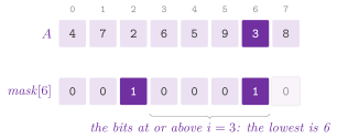
Lemma 6.25. Inside a block, the leftmost minimum of \(A[ i .. j ]\) is the place of the lowest set bit of \(\mathit{mask}[ j ]\) at or above \(i\), i.e., \(b + \mathrm{ctz}( \mathit{mask}[ j ] \wedge \neg ( 2^{i-b} - 1 ) )\). Moreover, \(\mathit{mask}[ j ] = ( \mathit{mask}[ j - 1 ] \wedge \neg G_j ) \vee 2^{j-b}\) for \(j > b\), where \(G_j\) has the bits of the places of the block larger than \(A[ j ]\), and a query makes at most five reads of the memory.
Proof. Let \(t^*\) be the leftmost minimum of \(A[ i .. j ]\). Since \(A[ t^* ] \le A[ u ]\) for each \(u\) in \(( t^* , j ]\), the bit of \(t^*\) is set by (6.14). A place \(t\) with \(i \le t < t^*\), instead, has \(A[ t ] > A[ t^* ]\), since \(t^*\) is the leftmost minimum, and its bit is not set, by (6.14) with \(u = t^*\). The lowest set bit at or above \(i\) is thus the bit of \(t^*\). As for the update, a place \(t < j\) is in the set (6.14) of \(j\) if and only if it is in that of \(j - 1\) and \(A[ t ] \le A[ j ]\), i.e., its bit is not in \(G_j\), and the place \(j\) always is. Finally, a query reads \(\mathit{mask}[ j ]\), the records of the places \(i\) and \(j\) (the minima of the suffix and of the prefix, with their offsets) and, across more than two blocks, two entries of the table. \(\square\)
A query across blocks takes the minimum of the suffix of the block of
\(i\), that of the prefix of the block of \(j\) and, if there are blocks in
between, that of the two entries of a sparse table on the minima of the
blocks that cover them, the leftmost of the smallest of three
(Algorithm 6.20). For each place, the minima of the suffixes and
of the prefixes are kept, with their offsets in the block
side by side, and so are the minima in the table, whose rows are built and
read by the same two functions as those of SparseTable (the doubling of
the rows and the two ranges that cover a query), on entries that keep the
minimum with its place instead of only the place. A query thus makes at
most five reads of the memory, independent of one another, and never reads
the array. Both answers (in one block and across blocks) are computed, and
one is chosen by a conditional move, which a random range would otherwise
mispredict half of the times.
Algorithm 6.20. The range minima by the
stacks in a word (after Baumstark et al.
2017); \(S\) is the table of the
minima of the blocks, as in SparseTable.
All the masks are built by the stacks in \(O( n )\) time or, on the integers
and the floating types under std::less, by one comparison of vectors of
the block per item (greaterBits()), by the update of
Lemma 6.25, with no branch. On fewer than \(2^{32}\) items,
the space is
bytes besides the array (the masks, the minima of the suffixes and of the
prefixes with their offsets, and the table), on huge pages, where \(p\) and
\(q\) are \(2 \, \mathrm{sizeof}( T ) + 2\) and \(\mathrm{sizeof}( T ) + 4\)
rounded up to the alignment of their records (12 and 8 for items of 32
bits). For a million items of 32 bits this is about 22 bytes per item,
against the \(8 ( \lfloor \log_2 n \rfloor + 1 ) = 160\) bytes per item of
the places of 64 bits of a SparseTable on all the items.
Table 6.3 summarizes the four structures.
Table 6.3. The structures of the range
minima in ADS/search.
| Structure | Preprocessing | Query | Source |
|---|---|---|---|
SparseTable |
\(O( n \log n )\) time and space | \(O( 1 )\) | Bender and Farach-Colton 2000 |
PlusMinusOneRangeMinimum |
\(O( n )\) | \(O( 1 )\), on steps of \(\pm 1\) | Bender and Farach-Colton 2000 |
RangeMinimum |
\(O( n )\) | \(O( 1 )\) | Bender and Farach-Colton 2000 |
WordRangeMinimum |
\(O( n )\), about 22 bytes per item of 32 bits | \(O( 1 )\), five reads at most | Baumstark et al. 2017 |
In ADS/search/RangeMinimum.h, the function is declared as
// declarations of <ADS/search/RangeMinimum.h>
template< class T , class Compare = std::less< T > >
std::vector< std::size_t > cartesianTree( const std::vector< T > & A ,
                                          Compare less = {} );
In ADS/search/RangeMinimum.h, the declarations of SparseTable and
PlusMinusOneRangeMinimum and RangeMinimum that a user calls are
// declarations of <ADS/search/RangeMinimum.h>
template< class T , class Compare = std::less< T > >
class SparseTable
{
 public:
 SparseTable( void );
 explicit SparseTable( std::vector< T > A , Compare less = {} );
 std::size_t query( std::size_t i , std::size_t j ) const;
 std::size_t size( void ) const;
 const T & operator[]( std::size_t i ) const;
 };
class PlusMinusOneRangeMinimum
{
 public:
 PlusMinusOneRangeMinimum( void );
 explicit PlusMinusOneRangeMinimum( std::vector< long > D );
 std::size_t query( std::size_t i , std::size_t j ) const;
 std::size_t size( void ) const;
 std::size_t blockSize( void ) const;
 };
template< class T , class Compare = std::less< T > >
class RangeMinimum
{
 public:
 RangeMinimum( void );
 explicit RangeMinimum( std::vector< T > A , Compare less = {} );
 std::size_t query( std::size_t i , std::size_t j ) const;
 std::size_t size( void ) const;
 const T & operator[]( std::size_t i ) const;
 const std::vector< std::size_t > & eulerTour( void ) const;
 };
In ADS/search/WordRangeMinimum.h, the declarations of WordRangeMinimum
that a user calls are
// declarations of <ADS/search/WordRangeMinimum.h>
template< class T , class Compare = std::less< T > >
class WordRangeMinimum
{
 public:
 WordRangeMinimum( void );
 explicit WordRangeMinimum( std::vector< T > A , Compare less = {} );
 std::size_t query( std::size_t i , std::size_t j ) const;
 std::size_t size( void ) const;
 const T & operator[]( std::size_t i ) const;
 };
6.10 The searches compared¶
The searches of the textbooks (binarySearch(), lowerBound(),
interpolationSearch(), the searches of Knuth, selection(),
SparseTable and RangeMinimum) are meant to show the methods and to
check their bounds. Instead, the engineered ones are meant to be compared with the
best implementations available, i.e., std::lower_bound for
branchlessLowerBound() and SPlusTree, the implementation of the paper
for the three PGM-indexes, std::nth_element for nthElement(), and the
structures of Baumstark et al. 2017
for WordRangeMinimum. Which search of a sorted array is fastest depends
(possibly more than on anything else) on whether the array fits in the
cache: on a small array the branch-free binary search usually wins, since
it has no structure to read, while on a large one the S+ tree and the
PGM-index read fewer lines, the latter in far less space on regular keys.
Their comparison on an idle machine, with the sizes of the arrays and the
distributions of the keys at which the ranking changes, belongs to
Appendix B.
6.11 Discussion and references¶
The binary search, the search by interpolation and the selection of Hoare are in Montresor 2025, §1.2, §12.1 and §17.1, the searches of Fibonacci and the uniform binary search in Knuth 1998, §6.2.1, and the unbounded searches in Bentley and Yao 1976; the expected cost of the interpolation is that of Perl et al. 1978. Khuong and Morin 2017 study the layouts of the arrays for the searches by comparison, and the S+ tree is that of Slotin 2022. The PGM-index, compressed and dynamic, is that of Ferragina and Vinciguerra 2020, on the optimal piecewise linear approximation of O'Rourke 1981 and Xie et al. 2014 and on the logarithmic method of Bentley and Saxe 1980. The bound of the minimum and the maximum together is that of Pohl 1972, the selection in linear time that of Blum et al. 1973; the sampling of Floyd and Rivest 1975 is analyzed by Kiwiel 2005, and the lower bound on the local minima of the hypercube is in Aldous 1983. The range minima follow Bender and Farach-Colton 2000, with the space of Fischer and Heun 2011 and the engineering of Baumstark et al. 2017; Ferragina 2023, chapter 10 uses them for the suffix arrays and the suffix trees.
The PGM-indexes, plain and compressed, are persistent
(§23.7): store() writes the keys and the
levels of the segments, and restoreMapped() reads them back, while the
type of the keys and the errors \(\epsilon\) and \(\epsilon_r\) are in the
file, and another instance of the template rejects it.
6.12 Exercises¶
Each exercise names the test of the library that solves it (run it with
ctest -R <name>).
- Find the minimum of a vector with \(n - 1\) comparisons (Montresor
2025, §1.2). Test:
ch01.sec1.2.min. - Realize the binary search with no overflow of the middle, and build its
decision tree, whose height is \(\lfloor \log_2 n \rfloor\). Tests:
ch01.sec1.2.binary-search,beyond.decision-tree,contract_search.binary-search. - Count the occurrences of a key in a sorted vector with two binary
searches (exercise 12.13), and find the first item not smaller than a
key in \(O( \log h )\) time if it is at the place \(h\) (exercise 12.9).
Tests:
ch12.ex12.13,ch12.ex12.9. - Realize the search by interpolation, and show a vector on which it
makes a linear number of probes. Tests:
ch12.sec12.1.interpolation,contract_search.interpolation-search. - Realize the Fibonacci search and the uniform binary search of Knuth.
Test:
taocp.knuth-searches. - Search a monotone predicate on the integers with no bound on its
answer, and compute the integer square root with no overflow and tell
the perfect squares. Tests:
lib_search.exponential-search,lib_search.integer-sqrt. - Find the minimum of a rotated vector, the item closest to a value, two
items with a given sum and the item of rank \(k\) of two sorted vectors.
Test:
lib_search.sorted-searches. - Find a peak and a local minimum of a vector, and a local minimum of a
binary tree, in a logarithmic number of comparisons. Tests:
lib_search.local-optima,contract_search.local-and-sorted. - Find the minimum and the maximum together with
\(\lceil 3 n / 2 \rceil - 2\) comparisons. Test:
contract_search.minimum. - Realize the selection of Hoare with a random pivot and the median of
the medians. Tests:
ch17.sec17.1.selection,contract_search.selection. - Realize the selection with the sample of Floyd and Rivest and the
partition of Lomuto with no branch, with the median of the medians
after too many rounds that cut little. Test:
ordered.nth-element. - Realize the binary search with no branch and the static B+-tree of
Slotin. Test:
ordered.static-search. - Realize the PGM-index, its compressed form with shared slopes, and its
dynamic form by the logarithmic method. Tests:
ordered.pgm-index,ordered.pgm-compressed,ordered.pgm-dynamic. - Answer the range minimum queries by the sparse table and by the
reduction of Bender and Farach-Colton. Test:
pearls_suffix.sec10.4.1.range-minimum. - Answer the range minimum queries by the stacks in a word, with at most
five reads of the memory per query. Test:
ordered.word-range-minimum.