7. Hashing and dictionaries¶
[Source: include/ADS/dictionary/DirectTable.h,
SortedArrayDictionary.h, HashFunctions.h, UniversalHashing.h,
RandomHashing.h, FastHash.h, RowFingerprint.h, TableSize.h,
ChainedHashTable.h, OpenHashTable.h, KnuthHashing.h,
FlatHashTable.h, DenseHashMap.h, PointerTable.h, PositionIndex.h,
CuckooHashing.h, BucketCuckooTable.h, PerfectHashing.h,
FingerprintPerfectHash.h, MinimalPerfectHash.h, RecSplit.h,
SkipList.h, IndexedSkipList.h, Trie.h, PatriciaTrie.h,
TwoLevelDictionary.h, AdaptiveRadixTree.h, SuccinctPatriciaTrie.h,
BinaryTrie.h, XFastTrie.h, YFastTrie.h, BitmapTrie.h]
We are concerned in this chapter with the DICTIONARY, i.e., a finite map
from a set of keys to a set of values that is searched by key, and with
its ordered variant, the SORTED SET of Morin 2013,
§1.2.4. This variant also answers for a
key \(x\) with the smallest key not smaller than \(x\). In ADS/dictionary
the first one is realized on a vector indexed by the key and
on a sorted vector (§7.2), and on the hash
tables of Montresor 2025, chapter 7
and of Morin 2013, chapter 5, with
their lists of overflow (§7.4) and their open
addressing (§7.5); the hash functions on
which all of them rest come first (§7.3). Beyond the
books, they add the engineered tables that compare the fingerprints of a
full group of places at once (§7.6), the
cuckoo hashing, whose searches look at two places in the worst case
(§7.7), and the perfect hashing of a static
set (§7.8). The ordered dictionaries follow:
the skip lists of Morin 2013, chapter 4
(§7.9), the digital search trees of strings
(§7.10) and those of the integers of \(w\)
bits of Morin 2013, chapter 13
(§7.11). In the last two, the searches
take a time that depends on the length of the key rather than on the
number of keys. The
three chapters of Morin are covered section by section, with each of his
lemmas, figures and exercises restated on the code of the library. The
exercises that ask to illustrate an operation are solved by the figures of
this chapter, and the others by the tests named in
§7.13. In the sets of
§1.9, AdaptiveRadixTree.h,
BucketCuckooTable.h, DenseHashMap.h, FastHash.h,
FingerprintPerfectHash.h, FlatHashTable.h, MinimalPerfectHash.h,
PointerTable.h, PositionIndex.h, RecSplit.h, RowFingerprint.h and
SuccinctPatriciaTrie.h are advanced and the other headers of this chapter
are base, while RandomHashing.h is in the core that the two sets include.
7.1 The interface¶
A DICTIONARY is a univocal relation from a set of keys to a set of values
(Montresor 2025, §3.2.3), with three
operations. Of these, lookup( k ) returns the value of the key \(k\) or
nothing, insert( k , v ) associates the value \(v\) to \(k\) (replacing the
value that \(k\) may have had), and remove( k ) removes \(k\) and its value if
\(k\) is there. Their meaning is fixed by the axioms
together with the two axioms which say that insert( k , v ) and
remove( k ) leave the value of each other key as it was. Realizations check
the first two as postconditions of their contracts, and the concept
Dictionary of ADS/ADT.h requires the three operations. Most realizations
also have contains( k ), size() and the iterators of the standard library
on their pairs, and the engineered ones a find( k ) that returns a pointer
to the value, to change it in place. The USET of Morin 2013,
§1.2.3 is a dictionary whose values are not
used. His SSET adds find( x ), the smallest key \(y \ge x\) (the successor
of \(x\)), which the ordered realizations of this chapter call
lowerBound( x ), after std::lower_bound, since their find( x ) is the
search of \(x\) itself. For the sets of Chapter 10,
ChainedHashTable, OpenHashTable, SortedArrayDictionary, SkipList and
IndexedSkipList also have findKey( k ), the address of the key \(k\) they
hold (nil if absent), and the last three lowerBoundKey( k ), the address of
the smallest key not smaller than \(k\) (nil if none), each valid until the key
is removed (or, in the hash tables, until the next change). These are the
operations that the concepts KeyedDictionary and OrderedDictionary of
SetInterfaces.h require and through which DictionarySet makes a USET or an
SSET of a dictionary, as described in Chapter 10.
All the realizations share a few conventions, which we state once. Each one
declares the types Key and Value (and Item, the keys, for the SSETs
of §7.11) and the types of the standard
library for its items, with begin(), end(), cbegin(), cend() and a
const_iterator, constant since a key may not change in place. The tables
whose items lie in places (DirectTable, OpenHashTable,
CuckooHashTable, BucketCuckooTable, the tables of Knuth,
PerfectHashTable and PointerTable) describe their places by a nested
Places, with size(), occupied() and read(), from which the
SlotIterator of ADS/Iterators.h (Chapter 1)
makes the iterator that skips the empty places. Their capacity() is the
number of places (of lists in ChainedHashTable, the stash excluded in
CuckooHashTable, 4 per bucket in BucketCuckooTable). Hash tables
take the hash as a template parameter H (std::hash for those of the
textbooks, DefaultHash for the engineered ones,
§7.3.6), and the engineered ones also an
equality Eq, std::equal_to by default. Contracts follow
ADS/Contract.h: the postconditions of (7.1) and the invariant of each
structure are checked at the levels stated in each section. An invariant
that costs a scan of the structure is checked in full only on small
structures (up to 1024 places, or 256 keys for the tries of integers), and
on the key of the operation beyond; hence, a long sequence of operations at
the contract level 3 stays linear.
Keys are drawn from a universe \(U\), and a dictionary holds \(n\) of
them at a time. When \(U\) is a small interval of integers, a vector with a
place for each key of \(U\) is enough (§7.2).
Otherwise a hash function \(H : U \rightarrow \{ 0 , \ldots , m - 1 \}\)
maps the keys to the \(m\) places of a table, and two distinct keys
\(k \ne k'\) with \(H( k ) = H( k' )\) make a collision. The table
must resolve it, either by lists of overflow (chaining,
§7.4) or by further places of the table itself
(open addressing, §7.5). Throughout the
chapter \(\alpha = n / m\) is the load factor of a table and \(h( k )\) is the
hash of a key, a word of 64 bits (or of the type std::size_t), from
which the place \(H( k )\) is computed, often as \(h( k ) \bmod m\). Also,
\(I( \alpha )\) and \(S( \alpha )\) are the expected numbers of places (or of
cells of a list) examined by an unsuccessful and by a successful search.
For the strings, \(\sigma\) is the size of the alphabet and \(|k|\) the length
of the key \(k\); for the integers, \(w\) is the number of bits of the keys.
A function \(H\) has the simple uniformity if each place receives the same share of the keys, weighted by the probability \(P( k )\) that the key \(k\) is in the dictionary (Montresor 2025, §7.1):
No fixed function satisfies (7.2) for each distribution of the keys (§7.3 shows why), and the analyses of the tables below therefore assume either (7.2) or, more honestly, a function drawn at random from a class whose properties are proved. The realizations differ in the time of the operations, in the space and in what they offer besides the three operations (the keys in order, a search by prefix, a static set), as Table 7.1 summarizes.
Table 7.1. The realizations of the
DICTIONARY and of the SORTED SET in ADS/dictionary, and the cost of their
operations; \(N\) is the total length of the keys of a trie, \(w\) the bits of
an integer key, and "expected" is over the choice of the hash function or
of the random levels.
| Realization | lookup |
insert, remove |
Space | Keys in order |
|---|---|---|---|---|
DirectTable |
\(O( 1 )\) | \(O( 1 )\) | \(\Theta( \vert U \vert )\) | yes |
SortedArrayDictionary |
\(O( \log n )\) | \(O( n )\) | \(\Theta( n )\) | yes |
ChainedHashTable |
\(O( 1 + \alpha )\) expected | as lookup, amortized if restructured |
\(\Theta( n + m )\) | no |
DLeftHashTable |
\(O( d \log \log n )\) w.h.p. | as lookup |
\(\Theta( n + m )\) | no |
OpenHashTable, CoalescedHashTable, BrentHashTable |
\(O( 1 / ( 1 - \alpha ) )\) expected | as lookup |
\(\Theta( m )\) | no |
FlatHashTable, DenseHashMap |
\(O( 1 )\) expected, \(\alpha \le 7 / 8\) | \(O( 1 )\) expected amortized | \(\Theta( m )\) | no |
CuckooHashTable, BucketCuckooTable |
\(O( 1 )\) worst case | \(O( 1 )\) expected amortized | \(\Theta( m )\) | no |
PerfectHashTable (static) |
\(O( 1 )\) worst case | built in \(O( n )\) expected | \(\Theta( n )\) | no |
SkipList, IndexedSkipList |
\(O( \log n )\) expected | \(O( \log n )\) expected | \(\Theta( n )\) expected | yes |
Trie, RadixTree |
\(O( \vert k \vert \log \sigma )\) | \(O( \vert k \vert \log \sigma )\) | \(O( N )\), \(O( n )\) nodes | yes |
AdaptiveRadixTree |
\(O( \vert k \vert )\) | \(O( \vert k \vert )\) | \(O( n )\) nodes and the keys | yes |
BinaryTrie, SimpleBinaryTrie |
\(O( w )\) | \(O( w )\) | \(O( n w )\) | yes |
XFastTrie, ListXFastTrie |
\(O( \log w )\) expected | \(O( w )\) expected | \(O( n w )\) | yes |
YFastTrie |
\(O( \log w )\) expected | \(O( \log w )\) expected amortized | \(O( n )\) | yes |
A table with direct access is preferable when \(| U |\) is of the order of \(n\), and the sorted vector when the lookups far outnumber the changes or the keys are wanted in order. A hash table fits the other cases, the engineered tables when the speed counts. Among the others, the cuckoo tables are usually the choice when the lookups must be fast in the worst case, and the perfect hashing when the set is static. Finally, the tries fit when the keys are strings to be searched by prefix or integers whose successors are wanted in time independent of \(n\).
7.2 Direct access and sorted vectors¶
When the keys are the integers of an interval \([ a , b ]\) of size \(m = b -
a + 1\), the function \(H( k ) = k - a\) is injective, i.e., a perfect hash in
the sense of §7.8. In this case the dictionary is a
vector \(A\) of \(m\) places, each empty or holding the value of its key
(Montresor 2025, chapter 7).
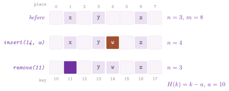
DirectTable realizes it with a counter \(n\) of the places not empty, which
its invariant checks (Algorithm 7.1, Figure
7.1); each operation costs \(O( 1 )\) time, while
the space is \(\Theta( m )\) whatever \(n\). Its contracts require \(a \le b\),
\(m\) places that fit in a std::size_t (which the full range of long does
not), and each key in \([ a , b ]\), a condition checked without overflow for
any long. Its iterators visit the places in order, and give the pairs \((
a + i , A[ i ] )\) of the places \(i\) not empty; hence the keys come out in
increasing order.
Algorithm 7.1. The operations of
DirectTable.
Below are the declarations of DirectTable, in the namespace ADS as all those of the chapter.
// declarations of <ADS/dictionary/DirectTable.h>
template< class V >
class DirectTable
{
 public:
 using Key = long;
 using Value = V;
 DirectTable( long a , long b );
 std::optional< V > lookup( long k ) const;
 void insert( long k , const V & v );
 void remove( long k );
 std::size_t size( void ) const;
 std::size_t capacity( void ) const;
 using const_iterator = SlotIterator< DirectTable , Places >;
 };
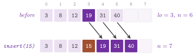
SortedArrayDictionary keeps the \(n\) pairs in a vector sorted by key, an
invariant (the keys strictly increasing) that its contracts check. A lookup
is the binary search of Montresor 2025,
§1.2, which finds the first place
\(\mathit{lo}\) whose key is not smaller than \(k\) in \(O( \log n )\) time (cf.
Chapter 6), whereas an insertion and a removal move
the pairs after \(\mathit{lo}\) one place to the right or to the left
(Algorithm 7.2, Figure
7.2). These take \(\Theta( n - \mathit{lo} )\)
moves, \(O( n )\) time, whereas the pairs come out in order at no cost and
the keys between two values are a range of places found by two binary
searches. A sorted vector is therefore preferable when the dictionary is built
once and searched often, and its pairs, contiguous and with no links, take
the least space of the realizations of this chapter.
Algorithm 7.2. The lookup and the
insertion of SortedArrayDictionary.
We declare SortedArrayDictionary as follows.
// declarations of <ADS/dictionary/SortedArrayDictionary.h>
template< std::totally_ordered K , class V >
class SortedArrayDictionary
{
 public:
 using Key = K;
 using Value = V;
 std::optional< V > lookup( const K & k ) const;
 void insert( const K & k , const V & v );
 void remove( const K & k );
 bool contains( const K & k ) const;
 std::optional< std::pair< K , V > > lowerBound( const K & k ) const;
 const K * findKey( const K & k ) const;
 const K * lowerBoundKey( const K & k ) const;
 bool empty( void ) const;
 std::size_t size( void ) const;
 const std::vector< std::pair< K , V > > & pairs( void ) const;
 using const_iterator = const std::pair< K , V > *;
 };
7.3 Hash functions¶
A hash table is only as good as its hash function: a function that sends the keys of the dictionary to few places makes each table of §7.4 to §7.7 a list. We now go through the functions of the area. Fixed ones of the textbooks come first, then the classes from which a function is drawn at random, the hash codes of the compound objects, and the engineered functions of 64 bits on which the tables of §7.6 rest.
7.3.1 The functions of a key¶
The functions of HashFunctions.h (Montresor 2025,
§7.1) read a key \(k\) as the string
\(\mathrm{bin}( k )\) of its bits, the bytes of a string one after the other
from the first, and the most significant bit of each first. In it, bin_bit()
gives one bit, and int_bin() the integer
\(\mathrm{int}( \mathrm{bin}( k ) )\) of a key of at most 8 characters.
Of these, the extraction (hash_extraction()) takes a block of \(p\) bits of
\(\mathrm{bin}( k )\) from a given place, and the XOR (hash_xor()) the
exclusive or of all the blocks of \(p\) bits, the last one padded with
zeros. Both give a place in \([ 0 , 2^p )\), and the second depends on
each bit of the key.
The division, \(H( k ) = \mathrm{int}( \mathrm{bin}( k ) ) \bmod m\), reads
the characters \(c_1 , \ldots , c_\ell\) of the key as the digits of a number
in a base \(\beta\) and computes it by the rule of Horner, taking the
remainder at each step (hash_division()). This gives the same result, since
\(( x \bmod m ) \beta + c \equiv x \beta + c \pmod{m}\), and no intermediate
value exceeds \(( m - 1 ) \beta + 255\), which the contract requires to fit in 64
bits. A leading digit (the seed) is allowed; hence, the familiar
\(h \gets 5\), \(h \gets 3 h + c\) is the base 3 with the seed 5.
In it, the remainder depends on all the bits of the key only if \(m\) is not a
power of 2 (otherwise it is the last \(\log_2 m\) bits of the last
characters). Montresor 2025, §7.1
recommends a prime far from a power of 2. A test of the simple uniformity
by the statistic \(\chi^2\) in ch07.sec7.1.uniformity shows the division
by a prime spreading random strings as a uniform distribution would, and
the extraction of the first bits sending the keys with a common prefix to
one place. A size \(m = 2^p - 1\) with characters of \(p\) bits is a trap of
its own: since \(2^p \equiv 1 \pmod{m}\), the hash is the sum of the
characters modulo \(m\), and any permutation of the characters of a key
gives the same place (Montresor 2025, exercise
7.8).
The multiplication reads the key as an integer \(i\) and takes
\(H( k ) = \lfloor m \, \mathrm{frac}( C i ) \rfloor\), with
\(\mathrm{frac}( y ) = y - \lfloor y \rfloor\). It works with any \(m\), and
for \(C = ( \sqrt{5} - 1 ) / 2\), the conjugate of the golden ratio, it
spreads the consecutive keys most evenly, since each point
\(\mathrm{frac}( C i )\), \(i = 1 , 2 , \ldots\), falls in one of the largest
gaps left by the points before it (Knuth 1998,
§6.4). In floating point
(hash_multiplication()) the formula is exact only while \(C i\) keeps
enough digits after the point, i.e., for \(i\) well below the \(2^{64}\) of
the mantissa of a long double. Its version of Knuth for \(m = 2^p\)
(hash_fibonacci()) works on integers instead: with
\(s = \lfloor C 2^{64} \rfloor\) and \(i s = r_1 2^{64} + r_0\), the place is
made of the \(p\) most significant bits of \(r_0\), i.e.,
\(\lfloor 2^p \, \mathrm{frac}( i s / 2^{64} ) \rfloor\), which differs from
the exact \(\lfloor m \, \mathrm{frac}( C i ) \rfloor\) by about
\(m i / 2^{64}\). The middle square (hash_midsquare()) takes the \(p\)
bits in the middle of the 64 least significant bits of \(i^2\).
In C++, the functions of HashFunctions.h are declared as follows.
// declarations of <ADS/dictionary/HashFunctions.h>
unsigned bin_bit( std::string_view k , std::size_t j );
std::uint64_t int_bin( std::string_view k );
std::uint64_t hash_extraction( std::string_view k , int p , std::size_t s );
std::uint64_t hash_xor( std::string_view k , int p );
std::uint64_t hash_division( std::string_view k , std::uint64_t m ,
                             std::uint64_t base = 256 ,
                             std::uint64_t seed = 0 );
std::uint64_t hash_multiplication( std::uint64_t i , std::uint64_t m ,
                                   long double C = ( std::sqrt( 5.0L ) - 1 ) /
                                                   2 );
std::uint64_t hash_fibonacci( std::uint64_t i , int p );
std::uint64_t hash_midsquare( std::uint64_t i , int p );
Each of these functions is fixed, and a fixed function, however good, has a set of keys on which it fails. If \(| U | > ( n - 1 ) m\), some place receives at least \(n\) keys of \(U\) by the pigeonhole principle, and a dictionary of those \(n\) keys is a single list. Hence the bounds in the worst case of the input need a function drawn at random after the keys are fixed, or, at least, a function whose choice the keys cannot depend on, which is the subject of the next subsections.
7.3.2 Universal classes¶
A class \(\mathcal{H}\) of functions \(U \rightarrow \{ 0 , \ldots , m - 1 \}\) is universal (Carter and Wegman 1979) if two distinct keys collide under at most a fraction \(1 / m\) of its functions,
and \(c\)-universal if \(c / m\) replaces \(1 / m\) in (7.3). By (7.3) and the
linearity of the expectation, the expected number of the other keys that
share the place of a key \(k\) is
\(\sum_{k' \ne k} \Pr[ H( k ) = H( k' ) ] \le ( n - 1 ) / m < \alpha\),
whatever the keys. Each bound of the chaining in
§7.4 thus holds in expectation over the
function, for each set of keys (Ferragina 2023,
chapter 8). UniversalHashing.h
has four classes of this kind.
Lemma 7.1. (Carter and Wegman.) With \(p\) a prime larger than the keys, the class \(\mathcal{H}_{p,m}\) of the functions \(h_{a,b}( k ) = ( ( a k + b ) \bmod p ) \bmod m\), \(1 \le a < p\) and \(0 \le b < p\), is universal.
Proof. For \(k \ne k'\), the map from \(( a , b )\) to \(( r , s ) = ( ( a k + b ) \bmod p , ( a k' + b ) \bmod p )\) is a bijection between the \(p ( p - 1 )\) pairs with \(a \ne 0\) and the pairs with \(r \ne s\): \(\mathbb{Z}_p\) is a field, and \(r - s = a ( k - k' )\) determines \(a\), and then \(r\) determines \(b\). For each \(r\), at most \(\lceil p / m \rceil - 1 \le ( p - 1 ) / m\) of the values \(s \ne r\) have \(s \equiv r \pmod{m}\); hence at most \(p ( p - 1 ) / m\) of the \(p ( p - 1 )\) functions make \(k\) and \(k'\) collide, which is (7.3). \(\square\)
CarterWegmanHash draws \(a\) and \(b\) from a seed with
\(p = 2^{61} - 1\), a Mersenne prime, and therefore the product \(a k \bmod p\) is
made of four products of 32 bits and a few shifts, with no integer of 128
bits (mulMod61() and mulMod() of ADS/numeric/NumberTheory.h,
Chapter 17). Its keys are below \(p\), and its
accessors p(), a(), b() and m() give the parameters. A similar
argument on the digits of a key gives DotProductHash,
\(h_a( k ) = \sum_i a_i k_i \bmod m\) for a prime \(m\), the key cut into its
\(r\) digits \(k_i\) in base \(m\) and \(a\) a vector of \(r\) random digits. If
two keys differ in the digit \(j\), the collision fixes \(a_j\) once the
other digits of \(a\) are chosen, since \(k_j - k'_j\) has an inverse modulo
\(m\), and the two keys collide under exactly \(m^{r-1} = | \mathcal{H} | / m\)
functions (universe() gives \(m^r\), or 0 past \(2^{64} - 1\)).
MultiplyShiftHash is the class of Dietzfelbinger et al.
1997, \(h_a( k ) = ( a k \bmod
2^h ) \operatorname{div} 2^{h - l}\) with \(a\) odd, for keys of \(h\) bits and
\(m = 2^l\). It is 2-universal, two keys colliding with probability at most
\(2 / m\) by an argument on the lowest bit in which they differ (the one of
Lemma 7.3 below). Also, it costs only a product
and a shift, the fastest of the classes (ofMultiplier() builds it from a
given \(a\)). StringHash turns a string into a key for the classes above,
by the polynomial \(\sum_i ( s_i + 1 ) x^i \bmod p\) of its characters at a
random point \(x\), \(p = 2^{61} - 1\). Each character counts one more, and
hence the character 0 counts too (the strings of zeros of different
lengths, or a string and the same followed by zeros, would collide
otherwise). Two distinct strings of length at most \(L\) collide with
probability at most \(L / ( p - 1 )\), since their difference is a polynomial
of degree at most \(L\), not zero, with at most \(L\) roots among the \(p - 1\)
points \(x \ne 0\) from which \(x\) is drawn (cf. Lemma
7.4 below). In the test
pearls_hashing.universal-classes we enumerate all the functions of small
classes and check the three bounds exactly.
Below are the declarations of the four universal classes.
// declarations of <ADS/dictionary/UniversalHashing.h>
class CarterWegmanHash
{
 public:
 explicit CarterWegmanHash( std::uint64_t m , std::uint64_t seed = 1 );
 CarterWegmanHash( std::uint64_t p , std::uint64_t a , std::uint64_t b ,
                   std::uint64_t m );
 std::uint64_t operator()( std::uint64_t k ) const;
 std::uint64_t p( void ) const;
 std::uint64_t a( void ) const;
 std::uint64_t b( void ) const;
 std::uint64_t m( void ) const;
 };
class DotProductHash
{
 public:
 DotProductHash( std::uint64_t m , int r , std::uint64_t seed = 1 );
 DotProductHash( std::uint64_t m , std::vector< std::uint64_t > a );
 std::uint64_t operator()( std::uint64_t k ) const;
 std::uint64_t universe( void ) const;
 };
class MultiplyShiftHash
{
 public:
 MultiplyShiftHash( int h , int l , std::uint64_t seed = 1 );
 static MultiplyShiftHash ofMultiplier( int h , int l , std::uint64_t a );
 std::uint64_t operator()( std::uint64_t k ) const;
 };
class StringHash
{
 public:
 explicit StringHash( std::uint64_t seed = 1 );
 std::uint64_t operator()( std::string_view s ) const;
 };
7.3.3 Multiplicative hashing on \(2^d\) places¶
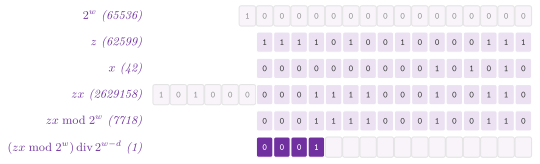
The tables of Morin 2013, chapter 5 keep \(m = 2^d\) places, \(d\) the dimension of the table, and take the place of a key from the high bits of a random function of its hash code \(x\) of \(w\) bits, rather than from \(x \bmod m\). The multiplicative hashing is
where \(a \operatorname{div} b = \lfloor a / b \rfloor\) and \(z\) is a random odd
integer of \(w\) bits (Dietzfelbinger et
al. 1997). Here the product modulo
\(2^w\) is what the arithmetic of the processor computes anyway, and the
division by \(2^{w-d}\) is a shift; Figure 7.3
follows (7.4) on a word of 16 bits. MultiplicativeHash realizes it with
\(w = 64\) on the hash code Code( k ) of the key (std::hash by default), the
multiplier from a seed or from ofMultiplier(). Its place( k , m ) is
(7.4), and makes it a PlaceHash of TableSize.h, i.e., a hash that maps a
key straight to a place of a table of \(2^d\) places, which ChainedHashTable
and OpenHashTable call in place of \(h( k ) \bmod m\). A table that grows and
shrinks keeps the same \(z\), and only \(d\) changes.
We declare MultiplicativeHash as follows.
// declarations of <ADS/dictionary/UniversalHashing.h>
template< class K = std::uint64_t , class Code = std::hash< K > >
class MultiplicativeHash
{
 public:
 explicit MultiplicativeHash( std::uint64_t seed = 1 , Code code = Code() );
 static MultiplicativeHash ofMultiplier( std::uint64_t z ,
                                         Code code = Code() );
 std::uint64_t operator()( const K & k ) const;
 std::size_t place( const K & k , std::size_t m ) const;
 std::uint64_t multiplier( void ) const;
 };
Its analysis rests on a fact of number theory, by which the products of a fixed odd number by the odd numbers modulo \(2^w\) are again all the odd numbers (Morin 2013, Lemma 5.3).
Lemma 7.2. Let \(O\) be the set of the odd integers in \(\{ 1 , \ldots , 2^w - 1 \}\), and \(q , i \in O\). Then exactly one \(z \in O\) has \(z q \bmod 2^w = i\).
Proof. Since \(O\) has as many choices of \(z\) as of \(i\), it suffices that two distinct \(z > z'\) of \(O\) never give the same product. If they did, \(( z - z' ) q \equiv 0 \pmod{2^w}\), i.e., the \(w\) lowest bits of \(( z - z' ) q\) would be 0. Yet, \(q\) is odd and \(0 < z - z' < 2^w\) has fewer than \(w\) trailing zeros; hence, their product has as many trailing zeros as \(z - z'\), fewer than \(w\). \(\square\)
Hence, if \(z\) is uniform on \(O\), so is \(z q \bmod 2^w\) for each odd \(q\): its lowest bit is 1 and its other \(w - 1\) bits are uniform and independent. This gives the bound on the collisions (Morin 2013, Lemma 5.1).
Lemma 7.3. For two distinct words \(x \ne y\) of \(w\) bits and \(z\) uniform on the odd words, \(\Pr[ \mathrm{hash}( x ) = \mathrm{hash}( y ) ] \le 2 / 2^d\).
Proof. The two hashes are the top \(d\) bits of \(z x \bmod 2^w\) and of \(z y \bmod 2^w\), and they agree only if the top \(d\) bits of the difference \(z ( x - y ) \bmod 2^w\) are all 0 (when the first product is the larger) or all 1 (when it is the smaller). Let \(( x - y ) \bmod 2^w = q 2^r\) with \(q\) odd. By Lemma 7.2, \(z q \bmod 2^w\) is 1 followed (upwards) by \(w - 1\) uniform bits, so that \(z ( x - y ) \bmod 2^w = z q 2^r \bmod 2^w\) has \(r\) zeros at the bottom, then a 1, then \(w - r - 1\) uniform bits. If \(r > w - d\), the top \(d\) bits hold both the 1 of the place \(r\) and the 0 of the place \(r - 1 \ge w - d\), and they are never all equal. If \(r = w - d\), the top \(d\) bits are the 1 and \(d - 1\) uniform bits, all 1 with probability \(2^{-( d - 1 )} = 2 / 2^d\). If \(r < w - d\), the top \(d\) bits are uniform, all 0 or all 1 with probability \(2 / 2^d\). \(\square\)
This bound is twice the \(1 / 2^d\)
of a random function, and it cannot be improved (Morin 2013, exercise
5.3). Indeed, for \(x = 2^{w-d-2}\) and \(y
= 3 x\), the products \(z x \bmod 2^w\) and \(3 z x \bmod 2^w\) depend only on
the \(d + 2\) lowest bits \(z'\) of \(z\). Then the two hashes are \(\lfloor z' / 4
\rfloor\) and \(\lfloor ( 3 z' \bmod 2^{d+2} ) / 4 \rfloor\), and since \(3 z'
= z' + 2 z'\) they agree for exactly 2 in \(2^d\) of the odd \(z'\). In the test ods_ints.ods5.1.multiplicative-hash we count the collisions of this pair on
\(2^{17}\) random multipliers. For a fixed \(z\) and \(n = 2^d\) with \(d \le w /
2\), on the other hand, \(n\) keys share a hash already by the pigeonhole
principle, \(2^w\) keys going to \(2^d\) places (Morin 2013, exercise
5.2), and they can be named. With
\(z^{-1}\) the inverse of the odd \(z\) modulo \(2^w\), the keys \(x_j = z^{-1} j
\bmod 2^w\), \(j = 0 , \ldots , 2^d - 1\), have the products \(z x_j \bmod 2^w
= j < 2^{w-d}\), which all hash to 0. (The test computes \(z^{-1}\) by the
iteration of Newton, \(y \gets y ( 2 - z y )\), each step doubling the bits
that are right.) The multiply-add hashing \(( ( z x + b ) \bmod 2^{2w} )
\operatorname{div} 2^{2w-d}\), with \(z\) and \(b\) random words of \(2 w\) bits,
has collision probability \(1 / 2^d\) (Dietzfelbinger
1996), at the price of products
of \(2 w\) bits.
7.3.4 Tabulation and random tables¶
Our analysis of the linear inspection in §7.5
assumes the places of the keys independent and uniform, which a table of \(2^w\)
random words indexed by the key would give, at a prohibitive space. The
simple tabulation of Carter and Wegman
1979 cuts a key of \(w\) bits into \(w / r\)
characters of \(r\) bits and keeps a table of \(2^r\) random words for each, the
hash being the XOR of the words of the characters. TabulationHash takes
\(w = 64\) and \(r = 8\), i.e., 8 tables of 256 words drawn from a seed (16 KB,
which typically stay in the cache of level 2). Its place( x , m ) takes the
top \(d\) bits of the hash on \(m = 2^d\) places, as the LinearHashTable of
Morin 2013, §5.2.3 does, which makes it a
PlaceHash too.
In C++, TabulationHash is declared as follows.
// declarations of <ADS/dictionary/RandomHashing.h>
class TabulationHash
{
 public:
 explicit TabulationHash( std::uint64_t seed = 1 );
 std::uint64_t operator()( std::uint64_t x ) const;
 std::size_t place( std::uint64_t x , std::size_t m ) const;
 };
With it, the hash of any key is uniform, since the word of one of its characters is, and those of two distinct keys are independent, since the keys differ in a character whose word appears in one hash only. Hence, the tabulation could thus replace the multiplicative hashing in the chaining. It is 3-independent but not 4-independent (the four keys \(( a , c )\), \(( a , d )\), \(( b , c )\), \(( b , d )\) of two characters have hashes whose XOR is 0), and therefore not a fully random function. Yet, Pătrașcu and Thorup 2012 proved that it gives the linear inspection, the cuckoo hashing and the minwise estimates the bounds of a fully random function, which is why the tables of this chapter that need independence use it.
Other tools of RandomHashing.h serve the tables and the searches of the
library. splitmix64() is the finalizer of the generator SplitMix64 of
Steele et al. 2014, a bijection of the
words of 64 bits made of steps that are each a bijection (a sum, a product by
an odd constant, or \(x \oplus ( x \gg s )\)). It mixes each input bit into each
output bit. SplitMix64 is the generator itself, a
UniformRandomBitGenerator (with min() and max()) whose state grows by
\(\lfloor 2^{64} / \phi \rfloor\) at each word and which seeds the tables and
the skip lists. fibonacciPlace( h , b ) takes the top \(b\) bits of
\(h \lfloor 2^{64} / \phi \rfloor \bmod 2^{64}\), the multiplicative hashing of
Knuth 1998, §6.4 with the golden ratio,
which spreads over a table of \(2^b\) places also the hashes whose low bits are
regular (cf. PointerTable in §7.6).
ZobristTable (Zobrist 1970) keeps a
random word \(R[ f ][ v ]\) for each feature \(f\) of a state and each value \(v\)
it may take, and the hash of a state is the XOR of the words of its pairs. Its
operator () gives one word, and hash( S ) the hash of a state given as any
range with access by index. A move that changes the value of a feature from
\(a\) to \(b\) updates the hash in \(O( 1 )\) time by two XOR,
\(h \oplus R[ f ][ a ] \oplus R[ f ][ b ]\) (update()), since \(y \oplus y = 0\)
takes the old word away. This makes it the hash of the board games and of the
states of a search, where the states are compared in a table of positions
already seen (cf. Chapter 19).
Below are the declarations of the other tools of RandomHashing.h.
// declarations of <ADS/dictionary/RandomHashing.h>
class SplitMix64
{
 public:
 using result_type = std::uint64_t;
 explicit constexpr SplitMix64( std::uint64_t seed = 0 );
 constexpr std::uint64_t operator()( void );
 static constexpr std::uint64_t min( void );
 static constexpr std::uint64_t max( void );
 };
class ZobristTable
{
 public:
 ZobristTable( std::size_t n , std::size_t m , std::uint64_t seed = 1 );
 std::uint64_t operator()( std::size_t f , std::size_t v ) const;
 template< std::ranges::random_access_range S >
  requires std::ranges::sized_range< S >
 std::uint64_t hash( const S & s ) const;
 std::uint64_t update( std::uint64_t h , std::size_t f , std::size_t a ,
                       std::size_t b ) const;
 };
constexpr std::uint64_t splitmix64( std::uint64_t x );
constexpr std::uint64_t fibonacciPlace( std::uint64_t h , int b );
7.3.5 Hash codes¶
Our tables work on keys of \(w\) bits, and a key that is not an integer (a
string, an array, an object of several parts) must first be mapped to such
a hash code (Morin 2013, §5.3). A
mapping of hash codes should have two properties. First, equal objects have
equal codes, and hence a key stored in a table is found by an equal one;
second, distinct objects have equal codes with probability close to \(1 /
2^w\), so that little is lost in the conversion. Primitive types of at most
\(w\) bits are their own codes (the bits read as an integer), and those of \(c
w\) bits, e.g., a long double, are compound objects of \(c\) parts. For a
compound object, the combinations of the codes of the parts by a XOR or by
a sum are easily foiled (we come back to this below). A sum of products by
random words, reduced by a multiplicative hashing on \(2 w\) bits, is not.
CompoundHash computes, for an object of \(r\) parts with the codes \(x_0 ,
\ldots , x_{r-1}\),
with \(w = 64\), the \(z_i\) random words and \(z\) a random odd integer of
\(2 w\) bits, all from a seed (parts() gives \(r\)).
We keep the sum on 128 bits, as two words with the carry, while only the high half of \(z s \bmod 2^{128}\) is wanted. This half the low halves of \(z\) and \(s\) give on 128 bits and the two crossed products only on their low 64 bits; hence, (7.5) costs \(r + 3\) products of words.
Theorem 7.1. (Morin 2013, Theorem 5.3.) If \(x_0 , \ldots , x_{r-1}\) and \(y_0 , \ldots , y_{r-1}\) are words of \(w\) bits with \(x_i \ne y_i\) for at least one \(i\), then \(\Pr[ h( x_0 , \ldots , x_{r-1} ) = h( y_0 , \ldots , y_{r-1} ) ] \le 3 / 2^w\).
Proof. Let \(h'( x ) = ( \sum_j z_j x_j ) \bmod 2^{2w}\) be the sum before the last step. Here \(h'( x ) = h'( y )\) reads \(z_i ( x_i - y_i ) \bmod 2^{2w} = t\), with \(t\) the sum of the terms \(z_j ( y_j - x_j )\) of the other \(j\), modulo \(2^{2w}\). Assume \(x_i > y_i\); then \(z_i ( x_i - y_i ) < 2^{2w}\), and therefore the equation is \(z_i ( x_i - y_i ) = t\), which has at most one solution \(z_i\); since \(z_i\) is independent of \(t\), it is that solution with probability at most \(1 / 2^w\). Otherwise \(h'( x ) \ne h'( y )\), two distinct words of \(2 w\) bits, which the multiplicative hashing of \(2 w\) bits into \(w\) bits sends to the same value with probability at most \(2 / 2^w\) by Lemma 7.3. The two cases give \(1 / 2^w + 2 / 2^w\). \(\square\)
This method needs a random word per part, and the arrays and the strings, whose length varies, take instead the polynomials over a prime field, which behave as the ordinary ones (Morin 2013, Theorem 5.4).
Lemma 7.4. Let \(p\) be a prime and \(f( z ) = x_0 + x_1 z + \cdots + x_{r-1} z^{r-1}\) a polynomial with coefficients in \(\{ 0 , \ldots , p - 1 \}\), not all 0. Then \(f( z ) \bmod p = 0\) has at most \(r - 1\) solutions \(z \in \{ 0 , \ldots , p - 1 \}\).
Proof. \(\mathbb{Z}_p\) is a field, in which a nonzero polynomial of degree \(e \le r - 1\) has at most \(e\) roots: each root \(z_0\) splits off a factor \(z - z_0\), by the division with remainder, and a field has no divisors of zero. \(\square\)
A sequence \(x_0 , \ldots , x_{r-1}\) with each \(x_i \le p - 2\) is then hashed at a random point \(z \in \{ 0 , \ldots , p - 1 \}\) by
whose last term is an end marker: \(p - 1\) is the item \(x_r\) of the sequence, different from each other item (Morin 2013, §5.3.3).
Theorem 7.2. Let \(p\) be a prime and two distinct sequences of items in \(\{ 0 , \ldots , p - 2 \}\), of lengths \(r\) and \(r'\). Then the probability that (7.6) gives them the same hash is at most \(\max\{ r , r' \} / p\), and at most \(( r - 1 ) / p\) when \(r = r'\).
Proof. If \(r = r'\) and \(x_i \ne y_i\) for some \(i\), the equality of the hashes is \(\sum_i ( x_i - y_i ) z^i \bmod p = 0\) (the end markers cancel), a nonzero polynomial of degree at most \(r - 1\). By Lemma 7.4 it has at most \(r - 1\) roots, i.e., it is satisfied by at most \(r - 1\) of the \(p\) values of \(z\). If \(r > r'\), the two sequences differ at the place \(r'\), where the shorter one has its end marker \(p - 1\) and the longer one an item \(x_{r'} \le p - 2\). In that case the difference of the hashes is a polynomial of degree \(r\) with the leading coefficient \(p - 1\), not zero, with at most \(r\) roots. \(\square\)
SequenceHash evaluates (7.6) by the rule of Horner from the end marker,
with \(p = 2^{61} - 1\), whose products mulMod61() reduces by shifts and
masks. Here the words of an array are first reduced to 60 bits by a
multiplicative hashing, and hence they lie below \(p - 1\). This costs a
collision probability of \(2 / 2^{60}\) more (two distinct arrays, the longer
of \(r\) words, collide with probability at most \(2 / 2^{60} + r / ( p - 1
)\)), while the bytes of a string are taken as they are (\(r / ( p - 1 )\)).
Both denominators are \(p - 1\) rather than the \(p\) of Theorem
7.2, since the point \(z\) is drawn from \(\{ 1 ,
\ldots , p - 1 \}\). Against the code of Morin 2013,
§5.3, which has \(w = 32\), the prime
\(2^{32} - 5\) and a division, the words are of 64 bits and the bounds are
\(2^{32}\) times smaller for the same work per word.
We declare the two hash codes as follows.
// declarations of <ADS/dictionary/UniversalHashing.h>
class CompoundHash
{
 public:
 explicit CompoundHash( std::size_t r , std::uint64_t seed = 1 );
 std::uint64_t operator()( std::span< const std::uint64_t > x ) const;
 std::size_t parts( void ) const;
 };
class SequenceHash
{
 public:
 explicit SequenceHash( std::uint64_t seed = 1 );
 std::uint64_t operator()( std::span< const std::uint64_t > x ) const;
 std::uint64_t operator()( std::string_view s ) const;
 };
Reducing modulo a Mersenne prime is the identity of Morin 2013,
exercise 5.10: with \(x = a 2^w + b\) and
\(2^w \equiv 1 \pmod{2^w - 1}\), one has \(x \equiv a + b\), and \(a + b < x\)
while \(x \ge 2^w\). Hence \(x \bmod ( 2^w - 1 )\) is the fixed point of
\(x \gets ( x \bmod 2^w ) + ( x \operatorname{div} 2^w )\), taken to 0 if it
is \(2^w - 1\), which is how mulMod61() reduces each product modulo \(p\)
in line 3 of the pseudocode above. Other
exercises of Morin 2013, §5.4 on the
hash codes are about why the easy combinations fail, and the answers are short.
A code that reads only the characters of even place, as the early
String.hashCode() of Java did on long strings, gives one code to the
\(2^{\ell / 2}\) strings of \(\ell\) characters that differ only in the others
(exercise 5.6). Also, the XOR of the two words of a pair gives 0 to each pair
\(( x , x )\), and their sum gives \(c\) to each pair \(( x , c - x )\)
(exercises 5.7 and 5.8). Each deterministic function of two words into
one has some value taken by at least \(2^{2w} / 2^w = 2^w\) pairs, by the
pigeonhole principle (exercise 5.9). In the test ods_ints.ods5.3.hash-codes
we check that CompoundHash and SequenceHash tell these sets apart, and
that the arrays of zeros of different lengths and the prefixes of an
array have distinct codes.
7.3.6 The engineered hash functions¶
Engineered tables, filters and perfect hash functions of the library use the
hashes of 64 bits of FastHash.h, made of the folded product, the product
\(a b\) of two words on 128 bits whose two halves are XORed,
\(( a b \bmod 2^{64} ) \oplus \lfloor a b / 2^{64} \rfloor\)
(foldedProduct()). It rests on product128(), which falls back to four
products of 32 bits where the compiler has no type of 128 bits. Each bit of
the folded product depends on each bit of the factors that the low half loses,
since the high half carries them, and a processor of 64 bits computes it by
one multiplication. A word thus costs one product, and a string one product
per 16 bytes (Thorup 2015 analyzes the
multiply-shift hashing on which this rests). hashWord( x , seed ) is the
folded product of \(x\) and of the seed XOR a constant.
hashBytes( p , n , seed ) hashes \(n\) bytes by their length, with no loop up
to 64 bytes. A string of at most 8 bytes is read as one word by two loads of 4
bytes at its ends (overlapping below 8) or by its first, middle and last byte
below 4 (the overlapping loads of the short tails of
wyhash). From 9 to 16 bytes, the product of
the two words that end at its ends; from 17 to 32 and from 33 to 64, two and
four products at once of its first and last blocks, folded by a last one. Past
64 bytes, out of line, the blocks of 16 bytes are folded into one state up to
96 bytes and into 6 independent states (a block of 96 bytes at a time) up to
256 bytes, the last 16 bytes with the length closing the hash. Past 256 bytes
the string is cut into stripes of 64 bytes, 8 lanes of a word each, as in
XXH3; the vectors of AVX2 or AVX-512
process 4 or 8 lanes at a time with the same result as the scalar code.
In C++, the hashes of FastHash.h are declared as follows.
// declarations of <ADS/dictionary/FastHash.h>
struct Product128
{
 std::uint64_t lo , hi;
 };
constexpr Product128 product128( std::uint64_t a , std::uint64_t b );
constexpr std::uint64_t foldedProduct( std::uint64_t a , std::uint64_t b );
constexpr std::uint64_t hashWord( std::uint64_t x , std::uint64_t seed = 0 );
std::uint64_t hashBytes( const void * p , std::size_t n ,
                         std::uint64_t seed = 0 );
template< class T >
struct FastHash;  // integers, enumerations, pointers, floating point
                  // numbers and strings: std::size_t operator()( x )
template< class K >
using DefaultHash = typename detail::DefaultHashOf< K >::type;
FastHash< T > is the hash of the integers, the enumerations, the pointers,
the floating point numbers (\(+0\) and \(-0\) hashing the same, since they are
equal) and the strings (std::string, std::string_view and the C strings,
which hash alike for the same characters), by hashWord() and hashBytes().
It declares the member type is_avalanching (the convention of Boost); hence,
FlatHashTable and the tables of Boost take its hash as it is, and the one of
the strings declares is_transparent, for the lookups by any string.
DefaultHash< K > is FastHash< K > when it is defined and std::hash< K >
otherwise (by the trait detail::DefaultHashOf), the default hash of the
engineered tables and filters (Product128 is the pair of halves of
product128()). kIndirectKey< K > is true when the hash of a K reads
memory that the key points to, as for the strings, and prefetchKey() then
brings the first line of that memory into the cache, which the rebuilds of the
tables use some keys ahead. We remark that a single product does not give the
full avalanche that the statistical batteries require (one bit of a key flips
each bit of the hash with probability near \(1 / 2\), not exactly \(1 / 2\)), and
that the functions are not cryptographic. Whoever knows the seed can make
collisions, and hence a table that faces adversarial keys must use a seed
drawn at random. A word is read in the byte order of the machine, so the
hashes differ between little and big endian machines. We check each path of
hashBytes() against known hashes in the test hashing.fast-hash, the same
with and without Highway, whose kernel of the stripes gives the words of
the scalar code.
RowFingerprint.h gives the fingerprints of 64 bits of the rows of
doubles, dense or sparse (the indices and the values in their order), for
finding the rows already seen, e.g., a cut generated twice, in a table of
the fingerprints (Rabin 1981). Values are compared as numbers, not as bit patterns: canonicalWord()
maps \(+0\) and \(-0\) to 0 and each NaN to one quiet NaN (IEEE
2019), and rowFingerprint() hashes the
canonical words a block of 64 at a time by hashBytes(). Each block is
seeded by the hash of the one before, and a sparse row hashes its indices
first, as bytes. Two rows with different words collide with probability
about \(2^{-64}\) for a hash that behaves at random, so that a table of \(k\)
fingerprints holds a false match with probability about \(k^2 2^{-65}\) by
the bound of the birthday problem. Since hashBytes() is not
cryptographic, sameRow() confirms a match in time linear in the row.
It first compares the bytes, which settles the common case of two
copies of the same row, and then, if some byte differs, it compares
the values as numbers.
Below are the declarations of the functions of RowFingerprint.h.
// declarations of <ADS/dictionary/RowFingerprint.h>
std::uint64_t canonicalWord( double x );
std::uint64_t rowFingerprint( std::span< const double > x ,
                              std::uint64_t seed = 0 );
template< class I >
std::uint64_t rowFingerprint( std::size_t n , const I * ind ,
                              const double * val ,
                              std::uint64_t seed = 0 );
bool sameRow( std::span< const double > a , std::span< const double > b );
template< class I >
bool sameRow( std::size_t na , const I * ia , const double * va ,
              std::size_t nb ,
              const I * ib , const double * vb );
7.4 Hash tables with lists of overflow¶
The table with lists of overflow (Montresor 2025,
§7.2.1; Morin 2013,
§5.1) goes back to an internal memorandum of
IBM of 1953 and to Peterson 1957. In it,
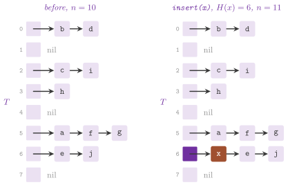
the place \(i\) of a vector \(T\) of \(m\) places holds the list of the pairs whose
keys have \(H( k ) = i\). ChainedHashTable keeps each list in the List of
ADS (Chapter 2), and insert() puts a new key at the
head of its list after a scan that rules out the key, while lookup() and
remove() go along the list (Algorithm 7.3,
Figure 7.4). Its template parameter Chain
chooses how a list is kept: FRONT, a new key at the head and nothing else
moves. MOVE_TO_FRONT, also the key found by lookup() goes to the head, and
hence the keys looked up often stay near it (Montresor 2025, exercise
7.5). SORTED, the keys of a list in
increasing order; hence, an unsuccessful search stops at the first larger key
(Montresor 2025, exercise 7.10). Its
place is \(H( k ) = h( k ) \bmod m\), or h.place( k , m ) for a PlaceHash
such as the multiplicative hashing of §7.3.3, on
a table of \(2^d\) lists.
Algorithm 7.3. The lookup and the
insertion of ChainedHashTable (Montresor 2025,
§§7.2.1 and 7.4); \(T[ 0 .. m - 1 ]\)
are the lists, and \(g\) is the load past which the table doubles.
We declare ChainedHashTable as follows, followed by an example of use.
// declarations of <ADS/dictionary/ChainedHashTable.h>
template< class K , class V , Chain C = Chain::FRONT ,
          class H = std::hash< K > >
 requires( C != Chain::SORTED || std::totally_ordered< K > )
class ChainedHashTable
{
 public:
 class const_iterator;
 using Key = K;
 using Value = V;
 explicit ChainedHashTable( std::size_t m , bool restructure = false ,
                            H h = H() );
 ChainedHashTable( std::size_t m , double g , double s , H h = H() );
 std::optional< V > lookup( const K & k ) const;
 void insert( const K & k , const V & v );
 void remove( const K & k );
 bool contains( const K & k ) const;
 const K * findKey( const K & k ) const;
 std::size_t size( void ) const;
 bool empty( void ) const;
 std::size_t capacity( void ) const;
 double load( void ) const;
 template< class F >
 void forEach( F && f ) const;
 std::vector< K > chain( std::size_t i ) const;
 std::size_t probes( void ) const;
 std::size_t restructures( void ) const;
 std::size_t moved( void ) const;
 };
ADS::ChainedHashTable< std::string , int > T( 8 );  // 8 lists
T.insert( "one" , 1 );
T.insert( "two" , 2 );
const std::optional< int > v = T.lookup( "two" );  // 2
T.remove( "one" );
Each scan of a list counts the cells it examines, the nil that ends an
unsuccessful search included, which probes() returns for the last
operation. Its code is the same for the three kinds of lists, but for the
test that stops a sorted list at the first larger key.
chain( i ) gives the keys of the list \(i\) from its head, forEach() visits
the pairs list after list in \(O( m + n )\) time (the foreach of the book), and
the iterators do the same, skipping the empty lists. With the load factor
\(\alpha = n / m\), the cost of a search is the following (Montresor 2025,
§7.3).
Lemma 7.5. Under the simple uniformity (7.2), or with a function drawn from a universal class, an unsuccessful and a successful search in a table with lists of overflow examine on average
cells, the nil that ends an unsuccessful search counted.
Proof. An unsuccessful search scans an entire list, of expected length \(\alpha\), and its end. A successful search of the key inserted \(j\)-th scans the keys inserted after it in its list, since each of them went to the head, i.e., \(( n - j ) / m\) of them on average, and then the key itself; the mean of \(1 + ( n - j ) / m\) over \(j = 1 , \ldots , n\) is \(1 + ( n - 1 ) / ( 2 m )\). \(\square\)
A list kept sorted stops an unsuccessful search, on average, halfway
through the list, and so does the scan that an insertion of keys in
random order makes first, while the successful search costs the same. The
test ch07.ex7.10 measures it, and ch07.sec7.3.complexity compares the
averages of (7.7) with those measured. Also, the multiplicative hashing of
§7.3.3 gives a bound of the same kind for
each set of keys, without (7.2) (Morin 2013,
Lemma 5.2).
Lemma 7.6. In a table of \(m \ge n\) lists
with the multiplicative hashing (7.4), the expected length of the list of
any key \(x\) is at most \(n_x + 2\), \(n_x\) being the number of the copies of
\(x\) in the table (0 or 1 in ChainedHashTable).
Proof. Let \(S\) be the keys of the table different from \(x\), and \(I_y\) the indicator of \(\mathrm{hash}( y ) = \mathrm{hash}( x )\) for \(y \in S\), whose expectation is at most \(2 / m\) by Lemma 7.3. The length of the list of \(x\) is \(n_x + \sum_{y \in S} I_y\), of expectation at most \(n_x + ( n - n_x ) \, 2 / m \le n_x + 2\), since \(m \ge n\). \(\square\)
A table may restructure itself (Montresor 2025,
§7.4): ChainedHashTable( m , true )
doubles \(m\) when \(\alpha\) exceeds \(g = 2\) and halves it, down to the
initial size, when \(\alpha\) falls below \(s = 1 / 2\), while
ChainedHashTable( m , g , s ) takes any two loads with \(g > 2 s \ge 0\).
Its new size is that of resized() of TableSize.h. A power of 2 doubles
or halves, while any other size goes to the first prime not smaller than its
double or its half (next_prime(), by trial divisions up to the square
root, is_prime()); hence, the inspections of
§7.5 that need a prime size keep working. By
the theorem of Chebyshev there is a prime between \(x\) and \(2 x\), and the
new size is therefore less than twice the one asked. is_pow2()
distinguishes the two cases.
In C++, the functions of TableSize.h are declared as follows.
// declarations of <ADS/dictionary/TableSize.h>
bool is_prime( std::size_t n );
std::size_t next_prime( std::size_t n );
bool is_pow2( std::size_t n );
std::size_t resized( std::size_t m , bool grow , std::size_t m0 );
Lemma 7.7. Let a table double its size when its load exceeds \(g\) and halve it, down to its initial size, when its load falls below \(s\), with \(g > 2 s\). Then any sequence of operations from an empty table costs \(O( 1 )\) amortized time per operation in the restructurings.
Proof. A restructuring of a table of \(m'\) places costs \(O( n + m' )
= O( m' )\) time, and it leaves the load near \(g / 2\) after a doubling and
near \(2 s\) after a halving, both strictly between \(s\) and \(g\) since
\(g > 2 s\). Within a constant factor, which the primes of resized()
change only by a constant, the next restructuring needs the load to grow
from there to \(g\) or to fall to \(s\), i.e., at least
\(\min\{ g / 2 - s , g - 2 s \} \, m' = \Omega( m' )\) insertions or
removals, which pay for it. \(\square\)
With the thresholds of the example of Montresor 2025,
§7.4, \(1 / 2\) and \(1 / 4\), a table
just doubled sits at the lower threshold, and a sequence that alternates an
insertion and a removal pays \(\Theta( m )\) per operation. This is why the
defaults are 4 times apart, as the test ch07.sec7.4.restructure checks on
such a sequence. restructures() and moved() count the restructurings
and the pairs they moved. With a PlaceHash, \(g = 1\) and \(s = 1 / 3\), the
table is the ChainedHashTable of Morin 2013,
§5.1, its lists in the List of ADS
instead of an array each. After a restructuring the load is about \(1 / 2\)
or \(2 / 3\), the lists are shorter (\(1 + \alpha \le 2\) cells per
unsuccessful search) at the price of a table up to twice as large. Then
Lemma 7.6 and Lemma
7.7 give the theorem of the book.
Theorem 7.3. (Morin 2013, Theorem
5.1.) The ChainedHashTable with the
multiplicative hashing, \(g = 1\) and \(s = 1 / 3\), realizes the USET (and
the DICTIONARY): ignoring the restructurings, insert(), remove() and
lookup() take \(O( 1 )\) expected time each, and any sequence of \(q\)
insertions and removals from an empty table spends \(O( q )\) time in all
the restructurings.
The bound of Lemma 7.5 is on the average list.
Yet, the longest list of a table with \(m = \Theta( n )\) lists has \(\Theta( \log
n / \log \log n )\) keys with high probability for a random function, and
\(O( \log n / \log \log n )\) in expectation for a universal class
(Ferragina 2023, chapter 8). In the test pearls_hashing.universal-chaining we measure both bounds on the
multiples of \(m\), which \(h( k ) = k \bmod m\) would put in one list.
DLeftHashTable in UniversalHashing.h shortens the longest list by
choice. It keeps \(d\) tables of \(w = \max\{ 1 , \lfloor m / d \rfloor \}\)
lists each, each table with a function of its own (a simple tabulation of
the hash of the key), and puts a key in the shortest of its \(d\) lists, the
leftmost one on a tie (Algorithm 7.4, Figure
7.5). A search looks at the \(d\) lists. For \(n =
m\) keys the longest list is then \(\ln \ln n / ( d \ln \phi_d ) + O( 1 )\)
with high probability, \(\phi_d\) being the growth rate of the generalized
Fibonacci numbers of order \(d\), against \(\Theta( \log n / \log \log n )\)
with one function. This is the power of two choices of Azar et al.
1999, with the asymmetric (leftmost)
tie-breaking of Vöcking 2003, an
exponential gain for one more probe; it allows each list to be a bucket of
fixed size \(O( \log \log n )\) instead of a linked list. For the simple
tabulation, Dahlgaard et al. 2016
proved a longest list of \(O( \log \log n )\) with high probability.
maxLoad() gives the length of the longest list and tables() the number
\(d\); the invariant, that each key is in one of its \(d\) lists and is counted
once, is checked on the key of the operation only past 1024 keys.
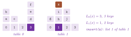
Algorithm 7.4. The insertion of
DLeftHashTable (Vöcking 2003).
Below are the declarations of DLeftHashTable.
// declarations of <ADS/dictionary/UniversalHashing.h>
template< class K , class V , class H = std::hash< K > >
class DLeftHashTable
{
 public:
 class const_iterator;
 using Key = K;
 using Value = V;
 DLeftHashTable( std::size_t m , int d , std::uint64_t seed = 1 , H h = H() );
 std::optional< V > lookup( const K & k ) const;
 void insert( const K & k , const V & v );
 void remove( const K & k );
 bool contains( const K & k ) const;
 std::size_t size( void ) const;
 std::size_t maxLoad( void ) const;
 int tables( void ) const;
 };
7.5 Open addressing¶
With open addressing (Montresor 2025,
§7.2.2) the pairs lie in the places
of the vector itself. A key \(k\) goes into the first free place of its
inspection \(H( k , 0 ) , H( k , 1 ) , \ldots , H( k , m - 1 )\), and a
search follows the same sequence until it meets \(k\) or a place that has
never been used. A place of OpenHashTable is in one of three states
(Slot): NIL, never used, which stops an inspection; FULL, holding a
pair. Finally, a DELETED place has been emptied by remove(); an
inspection goes past it and an insertion reuses it, since emptying the
place would cut the inspection of the keys placed after it. Hence \(\alpha <
1\), and the cost of a search depends on how the inspections of different
keys overlap. The scan of Montresor 2025,
§7.2.2 stops at the key, at a nil
place or after \(m\) inspections, and, for an insertion, remembers the first
deleted place met, where the new key goes if it is not found (Algorithm
7.5, Figure 7.6).
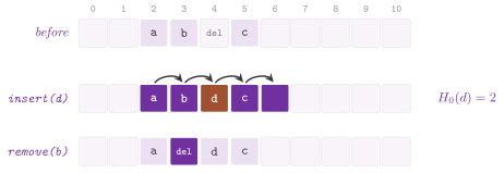
Algorithm 7.5. The scan, the lookup and
the insertion of OpenHashTable (Montresor 2025,
§§7.2.2 and 7.4); \(T[ 0 .. m - 1 ]\)
are the places.
We declare OpenHashTable as follows.
// declarations of <ADS/dictionary/OpenHashTable.h>
template< class K , class V , class H = std::hash< K > >
class OpenHashTable
{
 public:
 using Key = K;
 using Value = V;
 enum class Slot { NIL , FULL , DELETED };
 OpenHashTable( std::size_t m , Probing probe , bool restructure = false ,
                H h = H() );
 std::optional< V > lookup( const K & k ) const;
 void insert( const K & k , const V & v );
 void remove( const K & k );
 bool contains( const K & k ) const;
 const K * findKey( const K & k ) const;
 std::size_t size( void ) const;
 bool empty( void ) const;
 std::size_t capacity( void ) const;
 double load( void ) const;
 template< class F >
 void forEach( F && f ) const;
 Slot slot( std::size_t i ) const;
 const K & keyAt( std::size_t i ) const;
 std::size_t probes( void ) const;
 std::size_t restructures( void ) const;
 std::size_t moved( void ) const;
 using const_iterator = SlotIterator< OpenHashTable , Places >;
 };
Our code of the scan adds a constant stride to the place when the
inspection has one (the linear inspection and the double hashing), instead
of computing \(H( k , i )\) from scratch, and it records the places examined
for probes(). This count is atomic, and hence the lookups of a constant
table from several threads at once do not race
(engineered.open-hash-readers).
An insertion whose inspection finds no place, which the quadratic inspection
allows while some place is free, is not a fault of the caller and throws
std::overflow_error. slot( i ) and keyAt( i ) read the state and the key
of a place, forEach() visits the pairs place after place in \(O( m )\) time,
and the iterators skip the places that are not full. Its invariant, checked at
the contract level 3, is that the first place of the inspection of each key
that holds it is its own place with no nil before it, and that size() and
the deleted places are counted right. On a table of more than 1024 places it
is checked on the inspection of the key of the operation only, up to its first
nil.
The inspections of Table 7.2 are the factories of
Probing, each of a Kind, with \(H_0( k ) = h( k ) \bmod m\) (or the place of
a PlaceHash): linear( delta ), quadratic( c1 , c2 ), double_hashing()
and double_hashing( g ), whose step comes from a second function \(g\) of the
hash (of the type Probing::Step), triangular() and
pseudo_random( seed ). Also, at() gives \(H( k , i )\) from \(h( k )\), and
step() the step of the double hashing, coprime with \(m\) when \(m\) is prime or
a power of 2, i.e., \(H_\delta( k ) = 1 + ( h( k ) \bmod ( m - 1 ) )\) for a
prime and \(( \lfloor h( k ) / m \rfloor \bmod m ) \lor 1\), an odd number, for
a power of 2. Finally, stride() gives the constant difference of two
consecutive places, 0 for the inspections that have none. kind() gives the
Kind of an inspection (LINEAR, QUADRATIC, DOUBLE, and so on), and
works( m ) checks whether the inspection is a valid one on \(m\) places, which
check() asserts.
Table 7.2. The inspections of
OpenHashTable and how they compare.
| Inspection | \(H( k , i )\) | Sizes \(m\) | Behavior |
|---|---|---|---|
| linear | \(( H_0( k ) + \delta i ) \bmod m\) | \(\gcd( \delta , m ) = 1\) | primary clustering, but consecutive places in the cache |
| quadratic | \(( H_0( k ) + c_1 i + c_2 i^2 ) \bmod m\) | prime | secondary clustering only; not a permutation |
| triangular | \(( H_0( k ) + i ( i + 1 ) / 2 ) \bmod m\) | a power of 2 | a permutation; secondary clustering only |
| double hashing | \(( H_0( k ) + H_\delta( k ) \, i ) \bmod m\) | prime or a power of 2 | close to uniform hashing |
| pseudo-random | \(( H_0( k ) + p_i ) \bmod m\) | any | no primary clustering |
Here \(p_0 = 0 , p_1 , \ldots , p_{m-1}\) is a fixed random permutation of \(0 , \ldots , m - 1\), drawn from the seed for each size \(m\); hence, the pseudo-random inspection works with any \(m\) and two keys with different \(H_0\) do not share the rest of their inspection. As a model of the analysis is the uniform hashing, in which the inspection of each key is a random permutation of the places, independent of the others (Knuth 1998, §6.4).
Lemma 7.8. Under the uniform hashing,
Proof. An unsuccessful search examines more than \(i\) places only if its first \(i\) places are full, which has probability \(\frac{n}{m} \cdot \frac{n - 1}{m - 1} \cdots \le \alpha^i\); hence \(I( \alpha ) = \sum_{i \ge 0} \Pr[ \text{more than } i ] \le \sum_{i \ge 0} \alpha^i\). A successful search of a key follows the inspection of its insertion, which was an unsuccessful search in a table of load \(j / m\) for the \(( j + 1 )\)-th key. Here the mean over \(j = 0 , \ldots , n - 1\) of \(m / ( m - j )\) is at most \(\frac{1}{\alpha} \int_0^\alpha \frac{dx}{1 - x}\), the second bound of (7.8). \(\square\)
In the linear inspection, the full places gather in runs, and a key that falls anywhere in a run lengthens it. This is the primary clustering, whose cost Knuth 1998, §6.4 computed exactly for random places, \(I( \alpha ) \approx \frac{1}{2} ( 1 + 1 / ( 1 - \alpha )^2 )\) and \(S( \alpha ) \approx \frac{1}{2} ( 1 + 1 / ( 1 - \alpha ) )\), against the \(1 / ( 1 - \alpha )\) and \(- \ln( 1 - \alpha ) / \alpha\) of the double hashing. Yet, its places are consecutive in memory, and at a moderate load it is usually the fastest in practice. Both the quadratic and the triangular inspections spread the keys of different \(H_0\), while the keys with the same \(H_0\) still share their entire inspection (secondary clustering). In contrast, the double hashing comes close to (7.8), since the inspections of two keys coincide only if both \(H_0\) and \(H_\delta\) do. Note that the quadratic inspection is not a permutation in general. With \(m = 11\), the inspection \(( k \bmod 11 + 3 i + i^2 ) \bmod 11\) of the key 7 visits only the places 7, 0, 6, 3, 2 and 5, and an insertion may fail while the place 8 is free (Montresor 2025, exercise 7.2). The triangular one is a permutation on a power of 2.
Lemma 7.9. If \(m\) is a power of 2, the places \(i ( i + 1 ) / 2 \bmod m\), \(0 \le i < m\), are distinct.
Proof. If \(i ( i + 1 ) / 2 \equiv j ( j + 1 ) / 2 \pmod{m}\) with \(0 \le j < i < m\), then \(( i - j ) ( i + j + 1 ) \equiv 0 \pmod{2 m}\). These two factors add up to \(2 i + 1\), which is odd, and therefore one of them is odd. Its companion is positive and below \(2 m\), and their product, whose factors 2 all come from the even one, cannot be a multiple of the power of 2 \(2 m\), a contradiction. \(\square\)
A table may restructure itself (Montresor 2025,
§7.4). It doubles \(m\) when the full
and deleted places are more than \(m / 2\), so that \(\alpha \le 1 / 2\) and
the deleted places go away, and halves it, down to the initial size, when
\(\alpha < 1 / 8\); the two thresholds are 4 times apart, by Lemma
7.7. A new size that the inspection does not
work with, a prime that divides the step of a linear inspection, is
replaced by the next prime that it works with. Since only a removal halves
\(m\), a table emptied may stay above its initial size. When the places in
use exceed \(m / 2\) because of the deleted ones, with at most \(m / 4\) keys,
the table is rebuilt at the same size instead. Then the deleted places go
away and at least \(m / 4\) insertions come before the next rebuild, and
hence the cost stays \(O( 1 )\) amortized without the doubling that a table
emptied by removals and refilled with other keys would otherwise repeat. As
in the chaining, restructures() and moved() count them.
With a PlaceHash, the places of the inspection come from \(H_0( k )\)
alone; hence, the double hashing degenerates into the linear inspection,
and the table with the linear inspection, the tabulation hashing of
§7.3.4 and the restructuring is the
LinearHashTable of Morin 2013, §5.2.
His table rebuilds when the full and deleted places, \(q\) in his notation,
exceed \(m / 2\), on the smallest \(2^d \ge 3 n\) places, and halves when
\(n < m / 8\). Ours sizes the new table on the doubling or on the keys, as
above, with the same invariant \(q \le m / 2\) on which the analysis rests.
We say that a run of length \(k\) starts at \(i\) when the places
\(i , \ldots , i + k - 1\) are not nil and the places \(i - 1\) and \(i + k\)
are (the indices modulo \(m\)). The \(q\) keys inserted since the last
rebuild are assumed to have independent places, uniform on the table, an
assumption that §7.3.4 justifies for the
tabulation hashing.
Lemma 7.10. (Morin 2013, Lemma 5.4, with the full formula of Stirling.) Let \(q \le m / 2\) keys have independent places, uniform on \(m\) places. The probability \(p_k\) that a run of length \(k\), \(0 < k < q\), starts at a given place is at most
Proof. If a run of length \(k\) starts at \(i\), exactly \(k\) keys have their places in \(\{ i , \ldots , i + k - 1 \}\), which has probability at most \(\binom{q}{k} ( k / m )^k ( 1 - k / m )^{q - k}\) (the condition on the places \(i - 1\) and \(i + k\) dropped), largest for the least \(m\), i.e., for \(m = 2 q\). Then the formula of Stirling, \(\sqrt{2 \pi n} ( n / e )^n \le n! \le \sqrt{2 \pi n} ( n / e )^n e^{1 / ( 12 n )}\), bounds the binomial by \(\sqrt{ q / ( 2 \pi k ( q - k ) ) } \, e^{1 / ( 12 q )} \, q^q / ( k^k ( q - k )^{q - k} )\), and with \(m = 2 q\) the rest of the product is \(( k / 2 q )^k ( ( 2 q - k ) / 2 q )^{q - k} \, q^q / ( k^k ( q - k )^{q - k} ) = 2^{-k} ( 1 + k / ( 2 ( q - k ) ) )^{q - k} \le 2^{-k} e^{k / 2}\), since \(( 1 + 1 / x )^x \le e\) for \(x > 0\). \(\square\)
Morin replaces \(r!\) by \(( r / e )^r\) and loses the factor \(O( 1 / \sqrt{k} )\), which (7.9) keeps (Morin 2013, exercise 5.4); for \(k = q\) the probability is \(( q / m )^q \le 2^{-q}\) directly. A search for an absent key starts at a random place, and if the place belongs to a run of length \(k\) it costs \(O( 1 + k )\). A run of length \(k\) is counted by each of its \(k\) places, so that the expected cost is \(O( 1 + \frac{1}{m} \sum_i \sum_k k^2 \Pr[ \text{a run of length } k \text{ starts at } i ] ) = O( 1 + \sum_k k^2 p_k ) = O( 1 )\), a series that decreases exponentially. An insertion costs as much, a successful search as much as the insertion that placed its key, and a removal as a search; with Lemma 7.7 for the rebuilds, this is the theorem of the book.
Theorem 7.4. (Morin 2013, Theorem
5.2.) The OpenHashTable with the
linear inspection, the restructuring and independent uniform places
realizes the USET: ignoring the rebuilds, insert(), remove() and
lookup() take \(O( 1 )\) expected time each, and any sequence of \(q\)
insertions and removals from an empty table spends \(O( q )\) time in all
the rebuilds.
Three exercises of Morin 2013, §5.4 call
for an explanation. For instance, the student numbers of a class of first
year students differ in their last two digits, which spread them over 100
places, while their first two digits are those of the year of their
registration, nearly the same for all (exercise 5.1). An insertion that
puts the key in the first nil place, skipping the deleted ones, makes a
table of \(n\) keys spend \(\Theta( n^2 )\) time on \(O( n )\) insertions and
removals of one key \(x\). Each insertion walks past the deleted places left
by the earlier copies of \(x\) in its run, \(i\) of them at the \(i\)-th one,
until the deleted places fill half of the table and a rebuild clears them,
\(\Theta( n )\) insertions later (exercise 5.5). This is why the scan above
reuses the first deleted place it meets. Finally, the keys of a table with
a fixed hash can be chosen to fall in one place, which makes each search
linear (exercise 5.11). Two examples are the multiples of the number of
buckets for the std::unordered_map of libstdc++, whose hash of the
integers is the identity, or the multiples of \(2^{20}\) for a table of at
most \(2^{20}\) places on std::hash and \(h( k ) \bmod m\). A random \(z\) or
random tables hide the places from whoever chooses the keys, an attack on
the servers of the web described by Crosby and Wallach
2003. In the test
ods_ints.ods5.1.chained-hash-table we insert the keys \(k \cdot 2^{20}\)
and check that the multiplicative hashing spreads them.
Two tables of Knuth 1998, §6.4 in
KnuthHashing.h go beyond the book, both without removal.
CoalescedHashTable (Algorithm 6.4C, with the cellar of Vitter
1982) keeps the lists of overflow in
the table itself. A key that collides is put in the empty place of largest
index, found by a pointer \(r\) that only goes down, and linked at the end
of the list of its place; hence, the lists may merge (coalesce). First, the places taken are those of a cellar beyond the \(m\) places addressed
by the hash. With a cellar of about 14 % of the table the searches are
nearly as fast as with separate lists, with no memory out of the table
(Algorithm 7.6, Figure
7.7). Its invariant, an audit, is that each key
is on the list of its place, and probes() counts the places of the last
lookup() or insert().
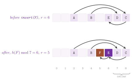
Algorithm 7.6. The insertion of
CoalescedHashTable (Knuth 1998, Algorithm
6.4C).
BrentHashTable is the double hashing on a prime \(m\) with the improvement of
Brent 1973 to the insertions. The new key
\(k\) is placed at the \(j\)-th place of its inspection, and the key found there
moved forward by \(s - j\) places of its own inspection, for the least \(s\), and
then the least \(j\), that find an empty place (Algorithm
7.7, Figure 7.8). Since
a successful search costs the place of its key in its inspection, the
insertion trades a long inspection of the new key for a short move of an old
one. In this way the expected number of probes of a successful search stays
below 2.5 even in a full table (Knuth 1998, exercise
6.4-49), against
\(- \ln( 1 - \alpha ) / \alpha\) of the plain double hashing, at no cost for the
searches. at( k , i ) gives the place \(i\) of the inspection of \(k\), and
probes() the places of the last lookup(). We check the bound at a load of
95 % in the test taocp.knuth-hashing.
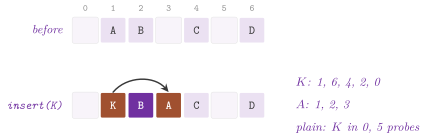
Algorithm 7.7. The insertion of
BrentHashTable (Brent 1973);
\(\mathrm{at}( x , i )\) is the place \(i\) of the inspection of \(x\) and \(i_y\)
the index of the key \(y\) in its own inspection.
In C++, the two tables of Knuth are declared as follows.
// declarations of <ADS/dictionary/KnuthHashing.h>
template< class K , class V , class H = std::hash< K > >
class CoalescedHashTable
{
 public:
 explicit CoalescedHashTable( std::size_t m , std::size_t cellar = 0 ,
                              H h = H() );
 std::optional< V > lookup( const K & k ) const;
 void insert( const K & k , const V & v );
 std::size_t size( void ) const;
 std::size_t probes( void ) const;
 using const_iterator = SlotIterator< CoalescedHashTable , Places >;
 };
template< class K , class V , class H = std::hash< K > >
class BrentHashTable
{
 public:
 explicit BrentHashTable( std::size_t m , H h = H() );
 std::optional< V > lookup( const K & k ) const;
 void insert( const K & k , const V & v );
 std::size_t size( void ) const;
 std::size_t probes( void ) const;
 using const_iterator = SlotIterator< BrentHashTable , Places >;
 };
7.6 Engineered hash tables¶
The tables of §7.4 and
§7.5 follow the textbooks, and their costs are
dominated by the misses of the cache rather than by the operations they
count. A list costs a pointer, i.e., a miss, per cell, and the linear
inspection compares entire keys along its run. Tables of this section are engineered on the layout of the Swiss tables of Kulukundis
2017 and of
boost::unordered_flat_map (Lopez Munoz
2022). Their places come in groups,
each with a control byte per place that holds a fingerprint of 8 bits of
the hash of its key; a search compares the fingerprint of its key with the
bytes of an entire group by one instruction,
and it touches the pairs only where
a fingerprint matches. Our benchmark of the dictionaries compares
FlatHashTable with boost::unordered_flat_map; we give no numbers here,
since they come from a campaign on an idle machine that is still to be run.
FlatHashTable keeps the places in groups of 15, after the Boost table.
Beside the vector of the pairs, each group has 16 bytes aligned to 16, one
control byte per place, empty (0) or full, in which case the byte is the
fingerprint of its key (never 0), and a 16th byte of overflow. The 15
control bytes are compared with the fingerprint of a key all at once, with
ADS_WITH_HIGHWAY by one comparison of the vectors of Google Highway
inlined at the instructions of the compiler (one of SSE2 on x86-64, of
NEON on ARM64), and otherwise by broadword operations on two words of 64
bits (Knuth 2011, §7.1.3). A macro,
ADS_FLAT_SIMD, defined as 0 before the header, selects the broadword
operations with Highway too. A
false match typically costs a comparison of keys and little else. Here the
hash \(h( k )\) is mixed as in Boost, by the folded product (mulx(), or
mulxPortable() by products of 32 bits) of \(h( k )\) and
\(\lfloor 2^{64} / \phi \rfloor\). Hence, each bit of the result depends on each
bit of \(h( k )\) and even the identity hash of the integers of std::hash
spreads over the table. A hash that declares is_avalanching on 64 bits, as
DefaultHash< K > does for the integers and the strings
(§7.3.6), is taken as it is. Then the top bits
of the mixed hash give the first group of the key, its low 8 bits the
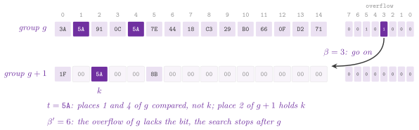
fingerprint \(t\) (1 in place of 0), and its low 3 bits the bit \(\beta\) of the
key in the bytes of overflow. The \(G\) groups, a power of 2, are inspected in
the triangular order \(g_i = ( g_0 + i ( i + 1 ) / 2 ) \bmod G\), a permutation
by Lemma 7.9 (Algorithm
7.8, Figure 7.9).
Algorithm 7.8. The lookup and the
insertion of FlatHashTable (the groups of Kulukundis
2017 and the overflow of Lopez
Munoz 2022); \(x\) is the mixed hash
of \(k\), \(m\) the number of places and \(d\) the bound of the places emptied
but still counted.
An insertion that goes past a full group sets the bit \(\beta\) of its key in
the overflow of that group, and a search stops at the first group whose
overflow lacks \(\beta\), after the places of that group whose fingerprint
matches. A search for an absent key thus reads, in the common case, one
group of 16 bytes (one line of the cache), and it never touches the
pairs.
remove() empties the place with no deleted mark. However, the bits of
overflow stay set until the next rebuild, and the searches keep going past
their group. We therefore call counted an empty place of a group whose
overflow is not 0, since it still counts as full. A removal adds 1 to a
bound \(d\) of the places counted with no load from memory (whether its place
is counted would take a read of the control bytes), and an insertion into
a counted place subtracts 1. Let \(b( m ) = m - \lfloor m / 8 \rfloor\), the
\(7 m / 8\) of the pseudocode rounded up. When \(n + d\) reaches \(b( m )\), the
places counted are counted exactly (deleted(), in \(O( m / 15 )\) time).
After this count the table is rebuilt only if fewer than \(m / 16\) places
are left below \(b( m )\): twice as large if the pairs exceed \(b( m ) / 2\), and of the
same size otherwise, in which case only the bits of overflow and the places
counted go away. These rules keep each inspection finite, as we now show.
Lemma 7.11. In a FlatHashTable (and in
the index of a DenseHashMap below), let \(D\) be the number of the places
counted. After each operation \(D \le d\) and \(n + d \le b( m )\); hence some
group has its overflow 0 and an empty place, each search stops, and each
insertion finds an empty place, within one visit of each group.
Proof. A place becomes counted only when a removal empties it in a group whose overflow is not 0, since an insertion that sets the first bit of a group finds the group full, with no empty place to count. Hence \(D\) grows by at most 1 at a removal, while \(d\) grows by 1; an insertion into a counted place lowers both by 1. A recount sets \(d = D\), a rebuild sets both to 0, and therefore \(D \le d\). A removal leaves \(n + d\) unchanged. An insertion that neither recounts nor rebuilds finds \(n + d < b( m )\), and one after a recount finds \(n + d + m / 16 < b( m )\); both raise \(n + d\) by at most 1. Finally, a rebuild at the same size leaves at most \(b( m ) / 2\) pairs, and a doubling at most \(b( m ) + 1 \le b( 2 m )\), with \(d = 0\). Thus the full places and those counted are at most \(n + D \le b( m ) < m\) (a table with places has at least 24 of them, and one with none searches a static group with no key and the overflow 0). Some place is therefore neither full nor counted, i.e., it is empty and its group has the overflow 0. The triangular order visits all the \(G\) groups (Lemma 7.9), and a search stops at that group at the latest, an insertion at its empty place. \(\square\)
The cost of an operation thus depends on how many groups have their overflow not 0, which the lemma bounds. As a model, in the manner of Lemma 7.8, we take the uniform hashing on the groups: the groups inspected for a key are a random permutation of the \(G\) groups, independent of the other keys, and its fingerprint is uniform on its 255 values and independent of its groups.
Lemma 7.12. Under the uniform hashing on
the groups, with \(s\) places per group (15 in a FlatHashTable, 12 in the
index of a DenseHashMap), a search for an absent key inspects at most 8
groups in expectation, and so do a search for a key of the table, its
removal and an insertion that does not rebuild. Besides the key that it
finds, a search compares at most \(8 s / 255 < 1 / 2\) keys in
expectation.
Proof. A search goes past a group only if the bit of its key is set in the overflow of the group, and an insertion only if the group is full. In both cases the group has no place that is neither full nor counted. By Lemma 7.11 there are at most \(F \le ( n + D ) / s \le b( m ) / s < 7 G / 8 + 1 / 8\) such groups. Since \(F\) is an integer and \(G \ge 2\) is a power of 2, \(F \le 7 G / 8\). The permutation of an absent key, or of the key of an insertion, is independent of the table, and its first \(i\) groups are all among the \(F\) with probability \(\frac{F}{G} \cdot \frac{F - 1}{G - 1} \cdots \le ( 7 / 8 )^i\); hence it inspects at most \(\sum_{i \ge 0} ( 7 / 8 )^i = 8\) groups in expectation. The insertion of a key of the table set its bit in each group that it went past, and the bit stays until the next rebuild, which inserts the key again. Hence the search of the key, and its removal, inspect the groups of that insertion, at most 8 in expectation. Finally, each of the at most \(s\) full places of a group inspected holds a key whose fingerprint equals that of the key searched with probability \(1 / 255\), and summing over at most 8 groups in expectation gives \(8 s / 255\). \(\square\)
Lemma 7.13. Any sequence of \(q\)
insertions and removals from an empty FlatHashTable (or DenseHashMap)
spends \(O( q )\) time in all the recounts and the rebuilds. Hence, under the
uniform hashing on the groups, each operation costs \(O( 1 )\) expected
amortized time.
Proof. A removal leaves \(n + d\) unchanged, and an insertion raises it by at most 1. A recount costs \(O( m )\), and when it does not rebuild it leaves \(n + d + m / 16 < b( m )\). Thus, the next recount comes at least \(m / 16\) insertions later, which pay for it. A rebuild into \(m'\) places costs \(O( m' )\) and leaves \(d = 0\) and at most \(b( m' ) / 2 + 2\) pairs: at most \(b( m ) / 2\) at the same size \(m' = m\), and at most \(b( m ) + 1 \le b( 2 m ) / 2 + 2\) after a doubling. The next rebuild needs \(n + d \ge b( m' )\) again, i.e., at least \(b( m' ) / 2 - 2 \ge m' / 4\) more insertions (since \(m' \ge 24\)), which pay for it. Finally, the second part follows from Lemma 7.12. \(\square\)
Some details of the engineering may be worth remarking, each of which the
header explains with the reason. When some fingerprint matches, the first line of the pairs of
the group is prefetched, at an address that depends only on the group, and
hence the two misses of a search overlap in part. A removal in the first
group of its key writes the 16 control bytes whole, at an address
that depends only on the hash. A store of a single byte would have an
address known only once the control bytes arrive, and the loads of the next
operations could not pass it (Intel
Corporation). A rebuild fills each new
group in the order of its places, keeping the counts of the groups apart, so
that it never reads a group it has just written. It also prefetches the
memory of a key that its hash reads 8 places ahead (Chen et al.
2004). Also, the new pair is built in the new
places before the old ones move; hence, a key or a value that lives in the
table is still there to copy. find() runs the entire inspection in line,
as Boost does, while the groups after the first and the rebuild are out of
line.
Its iterators visit the pairs in the order of the places, a group at a time by
the mask of its full places, and skip the empty groups whole up to a sentinel
group after the last. Hence, a step tests no bound (Algorithm
7.9). erase( it ) removes a pair and returns the
iterator on the next one. A removal moves no other pair and keeps the
iterators valid but the one on the removed pair. Instead, an insertion of a
new key that rebuilds the table invalidates them all. reserve( n ) makes
room for \(n\) pairs, clear() keeps the places, and capacity(), load(),
forEach() and swap() have their usual meaning. try_emplace( k , a... )
is the search of insert() followed, when \(k\) is not there, by the
construction of its value from a... in the new place; it returns a pointer
to the value and whether \(k\) was new, as std::unordered_map does with an
iterator, and leaves a... untouched when \(k\) is there. Hence, a value that
is read and then changed (e.g., the place of the last message of a key in an
outbox of Mailbox, §25.15) costs one inspection,
and DenseHashMap has the same member.
Algorithm 7.9. The step of the iterator of
FlatHashTable; \(M\) is the mask of the full places of the group \(g\) from
the current one on, its lowest bit the current place.
Below are the declarations of FlatHashTable, followed by an example of use.
// declarations of <ADS/dictionary/FlatHashTable.h>
template< class K , class V , class H = DefaultHash< K > ,
          class Eq = std::equal_to< K > ,
          class A = std::allocator< std::pair< const K , V > > >
class FlatHashTable
{
 public:
 using Key = K;
 using Value = V;
 explicit FlatHashTable( std::size_t n = 0 , H h = H() , Eq eq = Eq() );
 FlatHashTable( std::size_t n , H h , Eq eq , const A & alloc );
 explicit FlatHashTable( const A & alloc );
 FlatHashTable( const FlatHashTable & o );
 FlatHashTable( const FlatHashTable & o , const A & alloc );
 FlatHashTable( FlatHashTable && o ) noexcept;
 FlatHashTable( FlatHashTable && o , const A & alloc );
 ~FlatHashTable();
 std::optional< V > lookup( const K & k ) const;
 const V * find( const K & k ) const;
 V * find( const K & k );
 bool insert( const K & k , const V & v );
 bool insert( K && k , V && v );
 template< class... Args >
 std::pair< V * , bool > try_emplace( const K & k , Args &&... a );
 template< class... Args >
 std::pair< V * , bool > try_emplace( K && k , Args &&... a );
 bool remove( const K & k );
 bool contains( const K & k ) const;
 std::size_t size( void ) const;
 bool empty( void ) const;
 std::size_t capacity( void ) const;
 double load( void ) const;
 std::size_t deleted( void ) const;
 void reserve( std::size_t n );
 void clear( void );
 template< class F >
 void forEach( F && f ) const;
 template< class F >
 void forEach( F && f );
 void swap( FlatHashTable & o ) noexcept;
 class const_iterator;
 const_iterator erase( const_iterator it );
 };
ADS::FlatHashTable< std::uint64_t , double > F;
F.insert( 7 , 0.5 );
if( double * p = F.find( 7 ) )
 *p += 1;                            // 1.5, in place
const bool there = F.contains( 8 );  // false
Backend of Boost. With ADS_WITH_BOOST defined (by the option of CMake
of the same name, which defines it whenever the headers of Boost 1.83 or
later are found, by the makefile, which does the same, or by hand), the pairs of FlatHashTable are those of boost::unordered_flat_map,
the table whose layout it follows and with which it is on a par on our
benchmark (ADS_FLATHASH_BOOST defined to 0 keeps the code of ADS, the one
that Lemma 7.11 describes). The interface and
the contracts are kept, but for three points. First, capacity() is the
number of places of Boost, which fills all of them up to 29 places. Also,
deleted() counts the places that Boost no longer offers to the insertions
(the difference between its maximum load after a rebuild and its maximum
load now, in \(O( 1 )\) time). Finally, the iterators are those of Boost,
which are forward, and hence a visit cannot go backwards.
DenseHashMap separates the pairs from the index (Hettinger
2012 describes the same layout of the
dictionaries of CPython). The pairs are the items \(0 , \ldots , n - 1\) of a
vector \(A\), in the order of their insertions up to the removals, while an
index of open addressing maps a key to the position of its pair in \(A\). A
visit of the pairs is then a scan of \(n\) contiguous pairs, with no empty
place in between (data() gives them), and the index is rebuilt from \(A\)
without moving a pair. Its price is one more access per search (the index,
then the pair) and iterators that an insertion or a removal may invalidate,
as for a vector. The index is made of groups of one line of cache, 64
bytes, i.e., 12 control bytes, as in FlatHashTable, 3 bytes never
matched, a byte of overflow and the 12 positions of 32 bits of the places,
all in the same line. Hence, a search typically costs one miss in the index
and one in the vector. A removal empties the place of the key and moves the
last pair of \(A\) into the position left free (a swap with the last and a
pop). Then the place of the last pair in the index, found by the inspection
of its key comparing the positions rather than the keys, takes the new
position (Algorithm 7.10, Figure
7.10). As for the places counted, the recount
and the rebuilds follow the rules of FlatHashTable (with \(m / 16\) and
\(b( m )\)), and Lemmas 7.11 to
7.13 hold with groups of 12 places; a removal
makes one more inspection, that of the key of the last pair, as a search
of a key of the table. Its space is \(16 n\) bytes for pairs of 16 bytes plus 64 bytes per
12 places of the index, about 5.3 bytes per place, at a load between \(7 /
16\) and \(7 / 8\) after the first growth if there are no removals (the index
never shrinks). There are fewer than \(2^{32}\)
pairs.
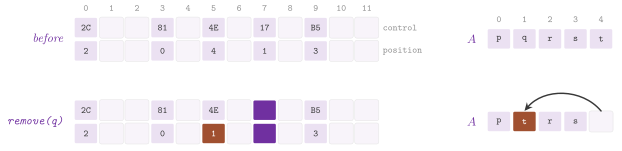
Algorithm 7.10. The lookup, the insertion
and the removal of DenseHashMap; \(A\) is the vector of the pairs and
\(g.\mathit{at}[ j ]\) the position of the place \(j\) of the group \(g\).
We declare DenseHashMap as follows.
// declarations of <ADS/dictionary/DenseHashMap.h>
template< class K , class V , class H = DefaultHash< K > ,
          class Eq = std::equal_to< K > ,
          class A = std::allocator< std::pair< const K , V > > >
class DenseHashMap
{
 public:
 using Key = K;
 using Value = V;
 explicit DenseHashMap( std::size_t n = 0 , H h = H() , Eq eq = Eq() ,
                        const A & alloc = A() );
 DenseHashMap( const DenseHashMap & o );
 DenseHashMap( const DenseHashMap & o , const A & alloc );
 DenseHashMap( DenseHashMap && o ) noexcept;
 DenseHashMap( DenseHashMap && o , const A & alloc );
 ~DenseHashMap() = default;
 std::optional< V > lookup( const K & k ) const;
 const V * find( const K & k ) const;
 V * find( const K & k );
 bool insert( const K & k , const V & v );
 bool insert( K && k , V && v );
 template< class... Args >
 std::pair< V * , bool > try_emplace( const K & k , Args &&... a );
 template< class... Args >
 std::pair< V * , bool > try_emplace( K && k , Args &&... a );
 bool remove( const K & k );
 bool contains( const K & k ) const;
 std::size_t size( void ) const;
 bool empty( void ) const;
 std::size_t capacity( void ) const;
 double load( void ) const;
 std::size_t deleted( void ) const;
 void reserve( std::size_t n );
 void clear( void );
 template< class F >
 void forEach( F && f ) const;
 const std::pair< K , V > * data( void ) const;
 void swap( DenseHashMap & o ) noexcept;
 using const_iterator =
   typename detail::AllocVector< A , std::pair< K , V > >::const_iterator;
 };
PointerTable is the closed list of a search, i.e., the set of the objects
already met (e.g., the nodes of the states of a search), each found from its
key. A place holds the pointer and the full hash of 64 bits of the key of its
object; hence, a probe compares two keys only when their hashes are equal and
a growth moves the places without touching the objects. Its inspection is
linear, along consecutive places and lines of cache, which usually beats the
lists of overflow when the table does not fit in the cache (Burns et
al. 2012). The first place of a hash is
fibonacciPlace(), so that the hashes whose low bits are regular (e.g., the
owner of a state in a parallel search, \(h \bmod p\)) still spread over the
table. Its load stays below \(7 / 10\), the table doubling past it; there is no
removal, which a search does not need. find_or_insert( key , hash , make )
inserts the object that make() returns only if the key is not there, with
one inspection (Algorithm 7.11, Figure
7.11). Its find() stops at the first empty
place, and prefetch( hash ) requests the first place of a hash, and hence
the misses of the lookups of all the successors of a node overlap. Two keys
are equal by eq( p , key ), by default StateEqual, i.e.,
p->state == key. Its places come from an allocator, which may give huge
pages (Chapter 5), and slotsFor( n ), the least power
of 2, at least 16, above \(10 n / 7\), gives the number of places that \(n\)
objects take. Hence, a table built with them or reserved by reserve( n )
never grows on the way; bytes() gives the memory of the places, and
capacity(), size(), clear() and forEach() have their usual meaning.
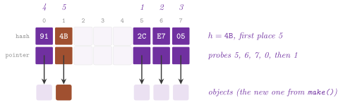
Algorithm 7.11. The search with insertion
of PointerTable (the linear inspection of Knuth 1998,
§6.4); \(S[ 0 .. m - 1 ]\) are the
places, \(m\) a power of 2.
In C++, PointerTable is declared as follows.
// declarations of <ADS/dictionary/PointerTable.h>
template< class T , class Eq = StateEqual ,
          class A = std::allocator< std::byte > >
class PointerTable
{
 public:
 explicit PointerTable( std::size_t capacity = 16 , Eq eq = Eq() ,
                        const A & alloc = A() );
 PointerTable( const PointerTable & ) = default;
 PointerTable( PointerTable && o ) noexcept;
 void clear( void );
 void reserve( std::size_t n );
 static constexpr std::size_t slotsFor( std::size_t n );
 template< class K , class Make >
 std::pair< T * , bool > find_or_insert( const K & key , std::uint64_t hash ,
                                        Make && make );
 template< class K >
 T * find( const K & key , std::uint64_t hash ) const;
 void prefetch( std::uint64_t hash ) const;
 std::size_t size( void ) const;
 std::size_t capacity( void ) const;
 std::size_t bytes( void ) const;
 template< class F >
 void forEach( F && f ) const;
 using const_iterator = SlotIterator< PointerTable , Places >;
 };
Backend of Boost. With ADS_WITH_BOOST defined, as for FlatHashTable
above, the places of PointerTable are those of boost::unordered_flat_set, which on
our benchmark of the dictionaries inserts and finds faster than the linear
inspection above (ADS_POINTERTABLE_BOOST defined to 0 keeps the code of
ADS). The class, its members and their signatures stay the same, and the
allocator is rebound to the places of Boost (a table on huge pages stays
on them). However, the load may reach \(7 / 8\), the maximum load of Boost,
and we give a table built with \(m\) places room for \(7 m / 10\) objects, as
many as the places of ADS hold; hence, a table of slotsFor( n ) places
still takes \(n\) objects with no growth, in about as many bytes. Also,
capacity() is then the number of places of Boost (\(15\) times a power of
2, less 1), the iterator is forward, and prefetch() does nothing, since
Boost offers no prefetch of the group of a hash.
PositionIndex maps the address of an object to its position, of 32 bits (the
type Position), in a vector that holds it, e.g., the constraints or the
variables of a model, whose positions change when some of them are erased. It
is a FlatHashTable from the address to the position, with the hash of ADS,
so that find(), insert() and erase() cost what they cost there. Its
NONE is the position of an absent key, contains() checks whether an
address is indexed, and assign( v ) indexes an entire vector of pointers,
\(v[ i ]\) at the position \(i\). Besides the operations of a dictionary,
renumber( E ) takes the sorted positions \(E\) just erased from the vector. In
one pass over the table, it drops the objects that were there and moves each
other position \(p\) to \(p - \mathrm{rank}( p )\), where
\(\mathrm{rank}( p ) = | \{ e \in E : e < p \} |\) (Algorithm
7.12, Figure 7.12).
In a bit vector of \(E\), the count \(\mathrm{rank}( p )\) is that of the erased
positions before the word of 64 bits of \(p\) plus the population count of the
bits of that word below \(p\), in \(O( 1 )\) time and with no branch (Jacobson
1989; cf. Chapter
22), and a position past the largest erased one moves
by \(| E |\). Since each word and its count sit side by side, a rank costs one
access to the memory; the keys of the erased positions are gathered on the way
and removed afterwards.
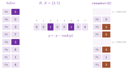
Algorithm 7.12. The renumbering of
PositionIndex; \(B\) is the bit vector of \(E\), \(w_j\) its words of 64 bits,
\(r_j\) the number of 1s in \(w_0 , \ldots , w_{j-1}\), \(N = \max E + 1\) and,
in this algorithm only, \(m = | E |\).
Lemma 7.14. Let \(E\) be sorted and with no
repetition. After renumber( E ) the index holds the objects whose positions
are not in \(E\), each at the position \(p - \mathrm{rank}( p )\) that it has in
the vector after the erasure, and the pass costs \(O( | E | + \max E / 64 )\)
time besides one visit of each place of the table and the \(| E |\) removals.
Proof. The erasure moves each object that stays down by the number of the objects erased before it, i.e., by \(\mathrm{rank}( p )\). For \(p < N\), the erased positions below \(p\) are those of the words \(w_0 , \ldots , w_{j-1}\), \(j = \lfloor p / 64 \rfloor\), which \(r_j\) counts, and those of \(w_j\) below the bit \(p \bmod 64\), which the population count of \(w_j \bmod 2^{p \bmod 64}\) counts (line 8). For \(p \ge N\), all of \(E\) is below \(p\) (line 5). An object goes to \(D\) exactly when the bit of its position is 1, i.e., when its position is in \(E\), and the removals come after the visit, which they therefore do not disturb. Building \(B\) and the counts \(r_j\) costs \(O( | E | + N / 64 )\), and each place \(O( 1 )\). \(\square\)
Below are the declarations of PositionIndex.
// declarations of <ADS/dictionary/PositionIndex.h>
template< class T , class H = FastHash< const T * > >
class PositionIndex
{
 public:
 using Position = std::uint32_t;
 static constexpr Position NONE = std::numeric_limits< Position >::max();
 explicit PositionIndex( std::size_t n = 0 , H h = H() );
 Position find( const T * p ) const;
 bool contains( const T * p ) const;
 bool insert( const T * p , Position i );
 bool erase( const T * p );
 template< std::ranges::random_access_range R >
 void assign( const R & v );
 void renumber( std::span< const Position > E );
 std::size_t size( void ) const;
 bool empty( void ) const;
 std::size_t capacity( void ) const;
 void reserve( std::size_t n );
 void clear( void );
 template< class F >
 void forEach( F && f ) const;
 void swap( PositionIndex & o ) noexcept;
 };
7.7 Cuckoo hashing¶
The cuckoo hashing of Pagh and Rodler
2004 gives each key \(k\) two places, \(h_1(
k )\) and \(h_2( k )\), of a table of \(m\) places, and keeps it in one of them.
Hence, a lookup and a removal look at two places, \(O( 1 )\) time in the
worst case. An insertion puts \(k\) in the first empty one of its two places,
else in \(h_1( k )\), evicting the key \(y\) there, which moves to its other
place, possibly evicting another key, and so on. After \(\mathit{MaxLoop}\)
evictions the insertion gives up and the table is rebuilt with two new
functions (a rehash). The cuckoo graph has the places as vertices and
an edge \(\{ h_1( k ) , h_2( k ) \}\) per key, and a placement of the keys is
an orientation of the edges in which each vertex receives at most one edge
(Ferragina 2023, chapter 8).
CuckooHashTable puts both functions on one table, and hence its graph is
a random graph of \(m\) vertices and \(n\) edges. It also adds a stash of \(s\)
places (Kirsch et al. 2009), which
keeps the keys whose insertion fails and which a search also looks at
(Algorithm 7.13, Figure
7.13).
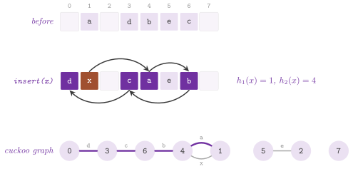
Algorithm 7.13. The insertion of
CuckooHashTable (Pagh and Rodler 2004;
Ferragina 2023, chapter 8); \(T\) is
the table, \(c\) the key in hand, and
\(\mathit{maxLoop} = \max\{ 8 \lceil \log_2 m \rceil + 16 , \lceil 3
\log_\gamma m \rceil \}\), with \(\gamma = 1 / ( 2\, \mathit{maxLoad} )\).
We declare CuckooHashTable as follows.
// declarations of <ADS/dictionary/CuckooHashing.h>
template< class K , class V , class H = std::hash< K > ,
          class A = std::allocator< std::pair< const K , V > > >
class CuckooHashTable
{
 public:
 using Key = K;
 using Value = V;
 explicit CuckooHashTable( std::size_t m = 16 , double maxLoad = 0.4 ,
                           std::size_t s = 0 , std::uint64_t seed = 1 ,
                           H h = H() , const A & alloc = A() );
 std::optional< V > lookup( const K & k ) const;
 void insert( const K & k , const V & v );
 void remove( const K & k );
 bool contains( const K & k ) const;
 std::size_t size( void ) const;
 std::size_t capacity( void ) const;
 std::size_t rehashes( void ) const;
 std::size_t evictions( void ) const;
 std::size_t stashed( void ) const;
 using const_iterator = SlotIterator< CuckooHashTable , Places >;
 };
The walk of the evictions (the loop of the insertion above) starts when the two places of the new key are full, and moves the key in hand to the other place of the key it evicts; in the cuckoo graph it follows the edges of the keys it moves. Whether it ends depends on the shape of the component of the new key.
Lemma 7.15. The keys can be placed if and only if each connected component of the cuckoo graph has at most one cycle, i.e., no more edges than vertices. Moreover, if the component of the new key has \(e\) edges (its key included) and at most one cycle, the walk of the evictions ends at an empty place after at most \(2 e\) evictions.
Proof. A component of \(v\) vertices and \(e\) edges can host its \(e\) keys in its \(v\) places only if \(e \le v\), i.e., if it is a tree or has a single cycle. Conversely, a tree oriented away from any vertex, and a cycle oriented around with the trees hanging from it oriented away from it, give each vertex at most one edge. As for the walk, the component has an empty place, since its \(e - 1\) old keys lie in its \(v \ge e\) places. The walk starts at the place \(h_1\) of the new key, and as long as it meets no place twice it follows a path, which ends if it reaches an empty place. Otherwise it meets a place already visited and closes the only cycle of the component. From there each key that it evicts goes back to the place it had before the walk, and the walk retraces its path back to \(h_1\), where it evicts the new key to \(h_2\). From \(h_2\) it follows a path that meets no place of the first part, since this would close a second cycle, and it ends at an empty place. Each edge is thus followed at most twice. \(\square\)
The probabilistic part rests on the random graph. As in the analysis of Pagh and Rodler 2004, the two places of each key are taken independent and uniform on the \(m\) places, and the bounds that follow do not depend on the two tables of their scheme.
Lemma 7.16. Let the \(n\) keys have their two places independent and uniform on the \(m\) places, with \(m \ge 2 c n\) for some \(c > 1\), and let \(x = 1 / c\). We have the following. (i) For two places \(i\) and \(j\) (possibly equal) and \(L \ge 1\), the cuckoo graph has a path (a cycle, if \(i = j\)) of \(L\) edges from \(i\) to \(j\) with probability at most \(x^L / m\). (ii) The component of a place has fewer than \(c / ( c - 1 )\) places in expectation, and an insertion that does not fail makes fewer than \(4 c / ( c - 1 )\) evictions in expectation. (iii) The graph has a cycle with probability at most \(1 / ( c - 1 )\), and a component with two cycles with probability at most \(4 x / ( ( 1 - x )^3 m )\).
Proof. (i) A path of \(L\) edges from \(i\) to \(j\) is fixed by its \(L - 1\) inner places, at most \(m^{L - 1}\) choices, and by its \(L\) keys in order, at most \(n^L\); the edge of a key joins two given places with probability at most \(2 / m^2\), independently of the other keys. Hence the probability is at most \(m^{L - 1} n^L ( 2 / m^2 )^L = ( 2 n / m )^L / m \le x^L / m\). (ii) A place \(j \ne i\) is in the component of \(i\) only if some path joins them, and by (i) the component has at most \(1 + ( m - 1 ) \sum_{L \ge 1} x^L / m < 1 + x / ( 1 - x ) = c / ( c - 1 )\) places in expectation. The component of a new key in the graph of the other keys, which satisfies the same hypothesis, is made of the components of its two places, which are independent of that graph; hence it has fewer than \(2 c / ( c - 1 )\) places in expectation. When it has at most one cycle it has no more edges than places, and Lemma 7.15 bounds the evictions by twice that. (iii) Summing (i) with \(i = j\) over the \(m\) places and the lengths gives \(\sum_{L \ge 1} x^L = 1 / ( c - 1 )\) for the cycles. A component with two cycles contains a connected subgraph with one edge more than its \(v\) places, made either of two cycles joined by a path (possibly with no edge) or of three paths between two places. Such a subgraph is fixed by at most \(( v + 2 )^2\) choices of the lengths of its cycles and paths, which add up to \(v + 1\). It is also fixed by its \(v\) places, at most \(m^v\) choices, and by its \(v + 1\) keys, at most \(n^{v+1}\). Its probability is thus at most \(\sum_{v \ge 1} ( v + 2 )^2 m^v n^{v+1} ( 2 / m^2 )^{v+1} \le \frac{1}{m} \sum_{j \ge 1} ( j + 1 )^2 x^j = \frac{x ( 4 - 3 x + x^2 )}{( 1 - x )^3 m}\), and \(4 - 3 x + x^2 < 4\). \(\square\)
With \(m = \Theta( n )\), a rehash at the end of \(n\) insertions thus needs an event of probability \(O( 1 / n )\) or a walk that the bound on \(\mathit{MaxLoop}\) cuts, and the classical result follows from these bounds.
Theorem 7.5. (Pagh and Rodler 2004; Ferragina 2023, chapter 8.) Let the cuckoo hashing use two tables of \(r \ge ( 1 + \epsilon ) n\) places each, functions of an \(O( \log n )\)-wise independent class, and \(\mathit{MaxLoop} = \lceil 3 \log_{1 + \epsilon} r \rceil\). Then a lookup and a removal take \(O( 1 )\) time in the worst case, and an insertion \(O( 1 )\) expected amortized time, the rehashes included, with a constant that depends on \(\epsilon\) alone.
With one table of \(m\) places, \(c = m / ( 2 n )\) plays the part of
\(1 + \epsilon\), and the code meets the hypotheses of Theorem
7.5 only in part; the theorem is therefore a
model of its behavior rather than a bound on it. First, both functions are
simple tabulations of the hash of the key, which Pătrașcu and Thorup
2012 proved to keep the failure
probability of the cuckoo hashing at \(O( 1 / n^{1/3} )\) (also, Aumüller
et al. 2014 give explicit families that
suffice with a stash). Second, the table doubles past the load maxLoad
(0.4 by default) and halves below \(\mathit{maxLoad} / 4\), the global
rebuilding of Ferragina 2023, chapter
8, and hence \(c \ge 1.25\). Third,
\(\mathit{MaxLoop}\) is the larger of \(8 \lceil \log_2 m \rceil + 16\) and
\(\lceil 3 \log_c m \rceil\) with \(c = 1 / ( 2\, \mathit{maxLoad} )\); the
first, which suits the small tables, falls below the second (about
\(9.32 \log_2 m\) by default) for \(m\) larger than about \(2^{12}\), so that the
hypothesis on \(\mathit{MaxLoop}\) holds at every size. The stash of \(s\) places
lowers the probability of a rehash from \(\Theta( 1 / n )\) to
\(\Theta( 1 / n^{s+1} )\) for random functions (Kirsch et al.
2009), and the test
pearls_hashing.cuckoo-analysis checks the evictions and the rehashes at
the loads 0.15 and 0.49, with and without a stash. rehashes(),
evictions() and stashed() count the rebuilds, the evictions and the
keys in the stash. Its invariant, that each key is in one of its places or
in the stash and is counted once, is checked on the key of the operation
only past 1024 places. Compared with the open addressing, a search has no
run to walk; the variants of today put several keys in a place (the
blocked cuckoo hashing, with loads above 90 %) or use \(d > 2\) functions
(Fotakis et al. 2005).
BucketCuckooTable is the first of these variants, the cuckoo hashing with
buckets of 4 places and a search in breadth of Li et al.
2014, the table of MemC3 (Fan et al.
2013) and of libcuckoo. A key with the hash
\(h\) may be in any of the 4 places of two buckets, and hence a search looks at
8 places in the worst case. In practice the table usually reaches a load of 95 % and more
before an insertion fails, against less than 50 % with one key per place.
(The analysis of the bins of constant size is that of Dietzfelbinger and
Weidling 2007.) Each place has a
tag of 8 bits, 0 when empty and otherwise 8 bits of the hash of its key
(1 in place of 0). All 4 tags of a bucket are a word of 32 bits, compared
with the tag of a key all at once by broadword operations, and therefore a
key is compared only in the places whose tag matches. The first bucket of a
key is given by the top bits of \(h\), and the second by the first and the
tag, \(b_2 = b_1 \oplus ( g( t ) \wedge ( B - 1 ) \vee 1 )\) for \(B\) buckets
(a power of 2) and a mixing \(g\) of the tag. This is the partial-key cuckoo
hashing of MemC3, an involution; hence, a key moves to its other bucket
with no need to hash it again.
An insertion puts a new key in a free place of its two buckets if any.
Otherwise it searches in breadth, from the places of its buckets, a path of
at most 5 moves that ends in a bucket with a free place (each key of a
bucket of the path moving to its other bucket). It then moves the keys along it
from the end, and the new key takes the first place of the path
(Algorithm 7.14, Figure
7.14). A search in breadth usually finds a
shorter path than the walk of the cuckoo hashing, and moves fewer keys.
When no path is found within 5 moves and 1024 buckets, or past the load of
98 %, the table doubles and each key is placed again. This costs \(O( 1 )\)
amortized per insertion as long as the failures come at a load bounded
away from 0, as they usually do (the doubling at the load \(\lambda\) moves
\(\lambda m\) keys, and the next one at the same load comes \(\lambda m\)
insertions later), but we have no bound on the load of a failure. For the keys whose hash reads memory, the doubling
hashes all the keys first, prefetching 8 keys ahead, and then places them,
prefetching 8 buckets ahead, so that the misses overlap (Chen et al.
2004). A removal clears the tag of its
place. load(), rehashes() and moves() report the load, the doublings
and the keys moved, and find() gives a value to change in place; an
insertion of a new key may move other keys and invalidates the iterators.
A concurrent version of the table, with a lock per region of buckets, is
in §24.7.
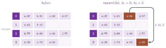
Algorithm 7.14. The insertion of
BucketCuckooTable (Li et al. 2014); \(b_1\)
and \(b_2\) are the two buckets of \(k\), and the search in breadth goes from a
bucket to the other buckets of its keys, at most 5 moves deep and 1024
buckets in all.
In C++, BucketCuckooTable is declared as follows.
// declarations of <ADS/dictionary/BucketCuckooTable.h>
template< class K , class V , class H = DefaultHash< K > ,
          class Eq = std::equal_to< K > ,
          class A = std::allocator< std::pair< const K , V > > >
class BucketCuckooTable
{
 public:
 using Key = K;
 using Value = V;
 explicit BucketCuckooTable( std::size_t n = 0 , H h = H() , Eq eq = Eq() ,
                             const A & alloc = A() );
 std::optional< V > lookup( const K & k ) const;
 const V * find( const K & k ) const;
 V * find( const K & k );
 bool insert( const K & k , const V & v );
 bool remove( const K & k );
 bool contains( const K & k ) const;
 std::size_t size( void ) const;
 bool empty( void ) const;
 std::size_t capacity( void ) const;
 double load( void ) const;
 std::size_t rehashes( void ) const;
 std::size_t moves( void ) const;
 using const_iterator = SlotIterator< BucketCuckooTable , Places >;
 };
7.8 Perfect hashing¶
A function is perfect on a set \(S\) of \(n\) keys if it has no collision on
\(S\), minimal if its range is \(\{ 0 , \ldots , n - 1 \}\), and order
preserving if it maps the keys in their order. A table built on a perfect
function searches in \(O( 1 )\) time in the worst case, as the table with
direct access of §7.2, but in space \(O( n )\)
instead of \(| U |\). Its price is that \(S\) is static, or changes at a cost
(the dynamic perfect hashing of Dietzfelbinger et al.
1994 inserts and removes in
\(O( 1 )\) amortized expected time). PerfectHashing.h has the two schemes
of Ferragina 2023, chapter 8, and
three more headers the compressed minimal perfect functions of today.
7.8.1 Two levels of universal hashing¶
PerfectHashTable is the scheme of Fredman et al.
1984. The \(n\) keys are hashed into \(n\)
lists by a function \(h\) of the class \(\mathcal{H}_{p,n}\) of Lemma
7.1 (CarterWegmanHash, with \(p = 2^{61} - 1\),
and hence the keys are integers below \(p\)). This function is drawn again
until \(\sum_j n_j^2 < 4 n\), \(n_j\) being the keys of the list \(j\). The list
\(j\) then becomes a table of \(n_j^2\) places with a function \(h_j\) of its
own, drawn again until it has no collision on the \(n_j\) keys (Algorithm
7.15, Figure
7.15). A search computes \(h\) and \(h_j\) and
compares one key, two accesses in the worst case.
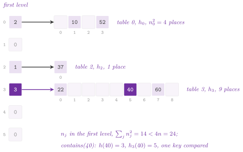
Algorithm 7.15. The construction of
PerfectHashTable (Fredman et al. 1984;
Ferragina 2023, chapter 8); \(n_j\)
is the number of the keys of \(S\) with \(h( k ) = j\).
Below are the declarations of PerfectHashTable, followed by an example of use.
// declarations of <ADS/dictionary/PerfectHashing.h>
class PerfectHashTable
{
 public:
 using Key = std::uint64_t;
 explicit PerfectHashTable( const std::vector< std::uint64_t > & S ,
                            std::uint64_t seed = 1 );
 bool contains( std::uint64_t k ) const;
 std::size_t size( void ) const;
 std::size_t space( void ) const;
 std::size_t trials( void ) const;
 using const_iterator = SlotIterator< PerfectHashTable , Places >;
 };
const std::vector< std::uint64_t > keys = { 10 , 22 , 37 , 40 , 52 , 60 };
const ADS::PerfectHashTable P( keys );
const bool in = P.contains( 40 );  // true
const ADS::MinimalPerfectHash< std::uint64_t > M( keys );
const std::size_t i = M( 37 );  // a place in [ 0 , 6 )
Lemma 7.17. (Fredman, Komlós and Szemerédi.) With \(h\) drawn from a universal class into \(n\) lists, \(E[ \sum_j n_j^2 ] < 2 n\), and the first level is drawn fewer than \(3 / 2\) times on average. A function drawn from a universal class into \(n_j^2\) places has no collision on \(n_j\) keys with probability more than \(1 / 2\). Hence the construction takes \(O( n )\) expected time and the second level fewer than \(4 n\) places.
Proof. One has \(\sum_j n_j^2 = n + 2 C\), \(C\) the number of the pairs of keys that collide, and by (7.3) \(E[ C ] \le \binom{n}{2} / n = ( n - 1 ) / 2\); hence \(E[ \sum_j n_j^2 ] \le 2 n - 1\). Also, the variable \(\sum_j n_j^2 - n = 2 C \ge 0\) has expectation below \(n\), and by the inequality of Markov it is at least \(3 n\), i.e., \(\sum_j n_j^2 \ge 4 n\), with probability below \(1 / 3\); the first level is thus accepted with probability above \(2 / 3\), after fewer than \(3 / 2\) draws on average. In the same way, \(n_j\) keys in \(n_j^2\) places collide in \(\binom{n_j}{2} / n_j^2 < 1 / 2\) pairs on average, and by the inequality of Markov they have no collision with probability more than \(1 / 2\). Each table of the second level is found after fewer than 2 draws on average, each draw costing \(O( n_j )\). \(\square\)
A threshold of \(2 n\), the mean itself, would be met with a probability
that the inequality of Markov does not bound away from 0, which is why the
code waits for \(4 n\); also, the 1000 draws of the first level after which
the build throws std::runtime_error all fail with probability below
\(3^{-1000}\) for distinct keys. space() gives the places of the second
level, \(\sum_j n_j^2\), and trials() the functions drawn by the build.
Each of the \(n\) buckets of the first level takes 6 words (the place of its
table, its size and the four words of its function \(h_j\)), and hence the
table has fewer than \(10 n + 4\) words in all; it gives nothing for a key out of \(S\) but a negative answer. In the test pearls_hashing.fks-example we replay the example of Ferragina 2023,
Figure 8.6. Today's compressed schemes need a few bits per key instead of words, and they rest on a lower
bound that the next lemma states.
Lemma 7.18. A family of functions from a universe of \(u\) keys into \(\{ 0 , \ldots , n - 1 \}\) that has a minimal perfect member for each set of \(n\) keys has at least \(\binom{u}{n} ( n / u )^n\) members. Hence, for \(u\) large with respect to \(n^2\), a minimal perfect hash function needs in the worst case at least \(n \log_2 e - O( \log n )\) bits, about 1.4427 bits per key.
Proof. A function \(f\) is minimal perfect on \(S\) only if \(S\) takes one key from each of the \(n\) preimages \(f^{-1}( i )\), i.e., on at most \(\prod_i | f^{-1}( i ) | \le ( u / n )^n\) sets, by the inequality between the arithmetic and the geometric mean; the family must cover the \(\binom{u}{n}\) sets. Since \(\binom{u}{n} \ge ( u - n )^n / n!\), the bound is at least \(( 1 - n / u )^n n^n / n!\), where the first factor tends to 1 when \(n^2 / u\) tends to 0, and \(\log_2 ( n^n / n! ) = n \log_2 e - \frac{1}{2} \log_2 ( 2 \pi n ) - o( 1 )\) by the formula of Stirling. A member of the family needs at least the logarithm of its size in bits. \(\square\)
Various schemes approach the bound at different costs, as Table 7.3 summarizes; the bits per key are those that the papers report, and those of the library are to be measured by the benchmarks.
Table 7.3. The minimal perfect hash functions of the area; \(\gamma\), \(\lambda\), \(b\) and \(\ell\) are the parameters of the schemes described below.
| Scheme | Header | Bits per key | Build | Evaluation |
|---|---|---|---|---|
| order preserving (Czech, Havas and Majewski) | PerfectHashing.h |
\(c \lceil \log_2 n \rceil\), \(c > 2\) or \(c > 1.23\) | \(O( n )\) expected | 2 or 3 accesses |
| fingerprints (BBHash, FMPH) | FingerprintPerfectHash.h |
\(\gamma e^{1 / \gamma}\), 3.3 for \(\gamma = 2\) | a few passes | \(e^{1 / \gamma}\) levels expected |
| pilots (PTHash) | MinimalPerfectHash.h |
about 3 | slower | 2 accesses |
| recursive splitting (RecSplit) | RecSplit.h |
about 1.8 | slowest, \(e^\ell\) per leaf | \(O( \log ( b / \ell ) )\) levels |
7.8.2 Order preserving functions on random graphs¶
OrderedMinimalPerfectHash is the scheme of Czech et al.
1992. Here \(r = 2\) functions map each key
\(t_i\) to the edge \(( h_1( t_i ) , h_2( t_i ) )\) of a random graph of \(m' =
c n\) vertices, labeled by the value wanted for \(t_i\), its place \(i\) in the
input (i.e., its rank, if the input is sorted). The function is \(h( t ) = (
g( h_1( t ) ) + g( h_2( t ) ) ) \bmod n\) for a labeling \(g\) of the vertices
that satisfies all the edges. If the graph is acyclic, a visit in depth of
each tree from its least vertex with \(g = 0\) assigns each other vertex
once, from the edge by which the visit reaches it (labelAcyclicGraph(),
Figure 7.16). The graph of \(n\) edges with
independent and uniform ends on \(c n\) vertices, \(c > 2\), is acyclic with a
probability that tends to \(\sqrt{( c - 2 ) / c}\) as \(n\) grows, i.e., about
\(\sqrt{3}\) graphs are drawn on average for \(c = 3\), the default. With \(r = 3\) functions into three
blocks of vertices the edges are triples of a hypergraph. These are solved
in the reverse order of its peeling, the repeated removal of a vertex of
degree 1 with its edge (labelByPeeling(), after Majewski et al.
1996). The peeling succeeds if the
hypergraph has no 2-core, i.e., with high probability for \(c > 1.23\), and
\(1.23 n\) values replace \(3 n\) (Algorithm
7.16).

Algorithm 7.16. The construction of
OrderedMinimalPerfectHash (Czech et al.
1992), the labeling of an acyclic graph
by visits in depth, and the labeling of a hypergraph by peeling, a vertex
of degree 1 knowing its edge as the XOR of the edges on it.
We declare OrderedMinimalPerfectHash as follows.
// declarations of <ADS/dictionary/PerfectHashing.h>
template< class K >
 requires( std::integral< K > ||
           std::convertible_to< const K & , std::string_view > )
class OrderedMinimalPerfectHash
{
 public:
 using Key = K;
 explicit OrderedMinimalPerfectHash( const std::vector< K > & keys ,
                                     int r = 2 ,
                                     double c = 0 , std::uint64_t seed = 1 );
 std::size_t operator()( const K & k ) const;
 std::size_t size( void ) const;
 std::size_t vertices( void ) const;
 std::size_t trials( void ) const;
 static std::optional< std::vector< std::uint32_t > >
 labelAcyclicGraph( std::size_t m , const std::vector< std::size_t > & E ,
                    const std::vector< std::size_t > & h , std::size_t n );
 static std::optional< std::vector< std::uint32_t > >
 labelByPeeling( std::size_t m , const std::vector< std::size_t > & E , int r ,
                 const std::vector< std::size_t > & h , std::size_t n );
 };
Lemma 7.19. If the graph is a forest, the labeling by visits satisfies each edge; if the hypergraph is peelable, the labeling in the reverse order of the peeling satisfies each edge. In both cases \(h( t_i ) = i\) for each key.
Proof. In a forest each edge joins a vertex to the one from which the visit reaches it, and the visit gives the second the label that satisfies the edge, \(g( v ) = ( i - g( u ) ) \bmod n\). No vertex is reached twice, since there is no cycle, and no edge is checked against a label already given. In the peeling, the vertex \(v\) removed with its edge \(e\) has degree 1 at that time; hence, the other vertices of \(e\) are removed later or never. In the reverse order, \(v\) is labeled after them, with the value that satisfies \(e\), and no edge labeled later contains \(v\), since all the edges on \(v\) but \(e\) were removed before \(e\). \(\square\)
It stores no key: \(O( m' )\) words, \(O( 1 )\) time to evaluate (vertices()
gives \(m'\), trials() the graphs drawn, and vertex() and
fingerprint() the vertex and the integer of a key for each function).
Unlike a trie (§7.10) it gives nothing
meaningful for a key out of \(S\). However, its space does not depend on the
length of the keys, which may be integers or strings, the latter turned
into integers by StringHash or splitmix64() before the functions of
Carter and Wegman. A build that draws 1000 graphs with no success throws
std::runtime_error, which for distinct keys and \(c = 3\) has a
probability that tends to \(( 1 - 1 / \sqrt{3} )^{1000} < 2^{-1000}\); the
test pearls_hashing.opmphf-example replays the
labeling of Ferragina 2023, Table 8.1.
7.8.3 Fingerprints, pilots and recursive splitting¶
FingerprintPerfectHash is the method of Müller et al.
2014, engineered as BBHash by
Limasset et al. 2017 and as FMPH by
Beling 2023. Keys go through
levels \(0 , 1 , \ldots\): the level \(i\) is a vector of
\(m_i = \lceil \gamma n_i \rceil\) bits for the \(n_i\) keys that reach it
(\(n_0 = n\), the sizes rounded up to blocks of 512 bits), each key hashed to
a place \(h_i( k )\) of it. The bit of a place is 1 if exactly one key falls
there, and the keys that share their place with others go to the next
level (Figure 7.17). A key is then mapped to
the number of 1s before its bit in the concatenation of the levels, which
is a bijection of \(S\) onto \(\{ 0 , \ldots , n - 1 \}\), since each key has
one bit of its own and each 1 belongs to one key. A key is alone in its
place with probability \(( 1 - 1 / m_i )^{n_i - 1} \approx e^{-1/\gamma}\),
so that
i.e., 3.30 bits per key for \(\gamma = 2\) and 2.72 (\(e\)) for \(\gamma = 1\), the least. A key of \(S\) goes through \(e^{1 / \gamma}\) levels in expectation, 1.65 for \(\gamma = 2\); hence, a smaller \(\gamma\) saves bits and costs levels, in the build and in the queries. The approximations of (7.10) become bounds, with constants slightly worse, as follows.
Lemma 7.20. Let the places of the keys at each level be independent and uniform, and let \(q = 1 - 4^{-1/\gamma}\). Then \(E[ n_{i+1} \mid n_i ] \le q n_i\), and hence \(E[ n_i ] \le q^i n\); the build has more than \(\ell\) levels with probability at most \(n q^\ell\), i.e., \(O( \log n )\) levels with high probability, and the levels take at most \(\gamma 4^{1/\gamma} n\) bits in expectation besides the rounding of each one to blocks of 512 bits.
Proof. A key of the level \(i\) is alone in its place with probability \(( 1 - 1 / m_i )^{n_i - 1}\). Since \(m_i \ge \gamma n_i\) and \(m_i \ge 512\), and \(( 1 - 1 / m )^m\) increases with \(m\) from the value \(1 / 4\) at \(m = 2\), this probability is at least \(( 1 - 1 / m_i )^{m_i / \gamma} \ge 4^{-1/\gamma}\), and a key goes on to the level \(i + 1\) with probability at most \(q\). Induction gives \(E[ n_i ] \le q^i n\), and the inequality of Markov gives \(\Pr[ n_\ell \ge 1 ] \le q^\ell n\). The level \(i\) takes at most \(\gamma n_i + 512\) bits, and \(\sum_i \gamma q^i n = \gamma n / ( 1 - q ) = \gamma 4^{1/\gamma} n\). \(\square\)
For \(\gamma = 2\) the lemma gives \(4 n\) bits against the \(3.30 n\) of (7.10), whose factor \(e^{-1/\gamma}\) is the limit of the probability that the proof bounds from below by \(4^{-1/\gamma}\).

Its build hashes each key once to a word \(x\) of 64 bits, and each level
hashes \(x\) again by a folded product with a constant of its own. A level is
two passes over its keys. The first one sets in a vector \(A\) the bit of each
place and in a vector \(C\) the bits of the places met twice, after which
\(A \gets A \wedge \lnot C\) a word at a time; the second one keeps the
keys whose
place is in \(C\) (Algorithm 7.17). Here the vectors of a level take \(2 \gamma n_i\) bits and stay in the cache of level 2 for a
million keys. A query computes \(h_0( k )\), tests its bit and, if it is 1,
gives its rank. The number of 1s before each block of 512 bits is kept in
32 bits, \(1 / 16\) of the bits more, and therefore a rank costs at most 8
counts of the bits of a word. bits() and levels() report the space and
the depth. Two keys with the same hash of 64 bits meet at each level and
cannot be separated, and the build then throws std::runtime_error.
Algorithm 7.17. The construction and the
evaluation of FingerprintPerfectHash (Müller et al.
2014); \(X\) are the hashes of the keys
still without a bit, \(A_i\) and \(C_i\) the bits of the level \(i\) and of its
places met twice, \(L\) the levels one after another and \(a_i\) the first bit
of the level \(i\).
In C++, FingerprintPerfectHash is declared as follows.
// declarations of <ADS/dictionary/FingerprintPerfectHash.h>
template< class T , class H = DefaultHash< T > >
class FingerprintPerfectHash
{
 public:
 using Key = T;
 explicit FingerprintPerfectHash( const std::vector< T > & keys ,
                                  double gamma = 2 , std::uint64_t seed = 1 ,
                                  H h = H() );
 std::size_t operator()( const T & k ) const;
 std::size_t size( void ) const;
 bool empty( void ) const;
 std::size_t bits( void ) const;
 std::size_t levels( void ) const;
 };
MinimalPerfectHash is the method of PTHash of Pibiri and Trani
2021, in the line of Fox et al.
1992 and of the compressed displacement of
Belazzougui et al. 2009. A key
with the hashes \(( h , h' )\) goes to the bucket \(b( h )\) of about \(n /
\lambda\) buckets, 60 % of the keys into 30 % of the buckets (the skewed
buckets of PTHash, so that the large buckets are placed while the table is
still empty). It also goes to the place \(p = \lfloor m \, g( h' \oplus
\pi_{b( h )} ) / 2^{64} \rfloor\) of a table of \(m = \lceil n / \alpha
\rceil\) places, where \(g\) is a folded product and \(\pi_b\) is the pilot of
the bucket, a product of the stored integer \(k_b\) by an odd constant. Its build places the buckets from the largest to the smallest, trying for each
one the integers \(k_b = 0 , 1 , 2 , \ldots\) until all its keys fall in free
places, distinct among them (Algorithm 7.18,
Figure 7.18). On average, the number of trials of
a bucket of \(s\) keys grows as \(1 / ( 1 - \text{load} )^s\), which is why the
larger buckets go first. The integers \(k_b\) are stored in \(\lceil \log_2 (
\max_b k_b + 1 ) \rceil\) bits each (the compact encoding of PTHash), and a
place \(p \ge n\) of a key is sent to one of the places below \(n\) left free,
by a table \(F\) of the \(m - n\) places beyond \(n\). An \(\alpha < 1\) makes the
search of the last buckets much faster, at the cost of this table. Searching the last buckets is the bottleneck of the build: with \(\alpha\)
near 1 some bucket may find no pilot within its limit; hence, \(\lambda\)
should stay below about 7 for \(\alpha = 0.99\), the defaults being \(\lambda
= 5\) and \(\alpha = 0.99\). A bucket that tries \(2^{24}\) pilots, or two keys
with the same hashes, make the build draw a new seed, and 100 seeds with no
success throw std::runtime_error; buckets(), trials() and bits()
report the buckets, the seeds drawn and the space. Both the parallel and
external construction of Pibiri and Trani
2024 and the optimized bucket sizes of
PHOBIC (Hermann et al. 2024) are not
done here.
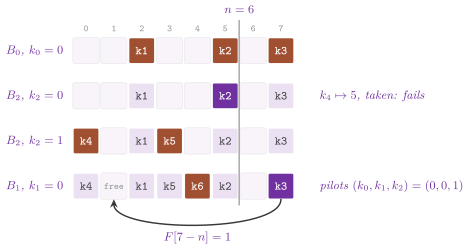
Algorithm 7.18. The construction and the
evaluation of MinimalPerfectHash (PTHash, Pibiri and Trani
2021); \(B_b\) are the second hashes of
the keys of the bucket \(b\), \(p( h' , k )\) the place of \(h'\) with the pilot
\(k\), and \(F\) the table of the free places below \(n\).
Below are the declarations of MinimalPerfectHash.
// declarations of <ADS/dictionary/MinimalPerfectHash.h>
template< class T , class H = DefaultHash< T > >
class MinimalPerfectHash
{
 public:
 using Key = T;
 explicit MinimalPerfectHash( const std::vector< T > & keys ,
                              double lambda = 5 ,
                              double alpha = 0.99 , std::uint64_t seed = 1 ,
                              H h = H() );
 std::size_t operator()( const T & k ) const;
 std::size_t size( void ) const;
 bool empty( void ) const;
 std::size_t bits( void ) const;
 std::size_t buckets( void ) const;
 std::size_t trials( void ) const;
 };
RecSplit is the method of Esposito et al.
2020, which comes closest to the bound
of Lemma 7.18. A key goes to the bucket
\(\lfloor h_1 \lceil n / b \rceil / 2^{64} \rfloor\) of \(\lceil n / b \rceil\)
buckets, \(b\) keys each on average (100 by default), by its first hash
\(h_1\). The \(m\) keys of a bucket are then split recursively by their
second hash \(h_2\), so that each leaf of the splitting tree holds at most
\(\ell\) keys (the template parameter L, 8 by default). A node of \(m\) keys
with the seed \(x\) sends a key to the place \(\rho_x = \lfloor g_{x,d}( h_2 )
\, m / 2^{64} \rfloor\), \(g_{x,d}\) a folded product salted by \(x\) and by the
depth \(d\), and its children by the place.
A leaf (\(m \le \ell\)) needs a
bijection, the seed for which the \(m\) places are distinct. A node of \(\ell
< m \le s \ell\) keys, \(s = \max\{ 2 , \lceil 0.35 \ell + 0.5 \rceil \}\)
(the lower aggregation), goes into parts of \(\ell\) keys. A node of \(s \ell
< m \le t s \ell\) keys, \(t = \lceil 0.21 \ell + 0.9 \rceil\) for \(\ell \ge
7\) and 2 below (the upper aggregation), goes into parts of \(s \ell\) keys; a
larger node goes into two parts of \(u = \lceil \lfloor m / 2 \rfloor / ( t
s \ell ) \rceil \, t s \ell\) and \(m - u\) keys (Algorithm
7.19, Figure
7.19). A node takes as seed the first \(x\) that
gives each part its size, a geometric variable of parameter
for the parts of \(k_0 , \ldots , k_{s-1}\) keys (a leaf being a node with \(m\) parts of one key, \(p = m! / m^m\)).
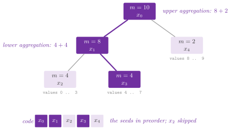
Lemma 7.21. (The invariance of RecSplit.) The product of the probabilities (7.11) of all the nodes of a splitting tree of \(m\) keys is \(m! / m^m\), whatever the shape of the tree.
Proof. By induction on the tree: a leaf is a node of \(m\) parts of one key, with probability \(m! / m^m\). A node with the parts \(k_0 , \ldots , k_{s-1}\) has the probability (7.11), and by induction its subtrees contribute \(\prod_i k_i! / k_i^{k_i}\); the product is \(\frac{m!}{\prod_i k_i!} \prod_i \frac{k_i^{k_i}}{m^{k_i}} \prod_i \frac{k_i!}{k_i^{k_i}} = \frac{m!}{m^m}\), since \(\sum_i k_i = m\). \(\square\)
The seeds are written in preorder by a code of Golomb 1966 and Rice, whose parameter for a geometric source of parameter \(p\) is the optimal one of Kiely 2004, \(r( p ) = \max\{ 0 , \lceil \log_2 ( - \log_2 \varphi / \log_2 ( 1 - p ) ) \rceil \}\) with \(\varphi\) the golden ratio, a function of \(m\) alone. Here a seed \(X\) is written as its \(r\) low bits followed by \(\lfloor X / 2^r \rfloor\) zeros and a one.
Lemma 7.22. Let \(X\) be geometric of parameter \(p\), \(\Pr[ X = x ] = ( 1 - p )^x p\) for \(x \ge 0\), \(0 < p < 1\). Its code of Golomb and Rice with the parameter \(r( p )\) has at most \(\log_2 ( 1 / p ) + 1 + \varphi + \log_2 \ln \varphi < \log_2 ( 1 / p ) + 1.563\) bits in expectation.
Proof. Since \(\Pr[ \lfloor X / 2^r \rfloor \ge j ] = \theta^j\) with \(\theta = ( 1 - p )^{2^r}\), the code has \(r + 1 + \theta / ( 1 - \theta )\) bits in expectation. Let \(L = \ln \varphi / ( - \ln ( 1 - p ) )\), so that \(r( p ) = \max\{ 0 , \lceil \log_2 L \rceil \}\), and note that \(L \le \ln \varphi / p\), since \(- \ln ( 1 - p ) \ge p\). If \(L > 1\), then \(2^r = \lambda L\) with \(1 \le \lambda < 2\), \(\theta = \varphi^{-\lambda}\), and the expectation is \(\log_2 L + 1 + \log_2 \lambda + 1 / ( \varphi^\lambda - 1 )\). On \([ 1 , 2 ]\) one has \(\log_2 \lambda \le \lambda - 1\), and \(\lambda - 1 + 1 / ( \varphi^\lambda - 1 )\) is convex, with the value \(1 / ( \varphi - 1 ) = \varphi\) at \(\lambda = 1\) and \(1 + 1 / ( \varphi^2 - 1 ) = \varphi\) at \(\lambda = 2\); hence the expectation is at most \(\log_2 L + 1 + \varphi \le \log_2 ( 1 / p ) + \log_2 \ln \varphi + 1 + \varphi\). If \(L \le 1\), i.e., \(p \ge 1 - 1 / \varphi = 1 / \varphi^2\), then \(r = 0\) and the expectation is \(1 / p\); the function \(y - \log_2 y\) of \(y = 1 / p\) is convex on \([ 1 , \varphi^2 ]\), and therefore at most \(\max\{ 1 , \varphi^2 - 2 \log_2 \varphi \} < 1.24\). \(\square\)
The bound is tight within 0.06 bits for small \(p\). Also, the code is never
longer than the entropy of \(X\) by more than 1.563 bits. By Lemma
7.21, a tree of \(m\) keys with \(t\) nodes with a
seed thus takes at most \(1.563 t + \log_2 ( m^m / m! ) \le 1.563 t + m
\log_2 e\) bits in expectation, the bound of Lemma
7.18 plus the price of the nodes. (The
rotations below make the seed of a leaf only approximately geometric of
parameter \(m! / m^m\), and for the leaves the bound is therefore a model.) The \(r( p )\)
low bits of all the seeds of a bucket come first, then all their unary
parts. Both tables RecSplitTables, computed once for each \(\ell\) and the
sizes \(m < 4096\), give \(r\), the low bits of a subtree and its number of
nodes. Hence, a subtree is skipped by moving a pointer on the low bits and
by a select on the unary parts (recSplitSelect(), the broadword select
of selectInWord(), §22.2). The numbers of keys
before each bucket and the places of their codes are two sequences of Elias
and Fano (Elias 1974; cf. Chapter
22), less their linear estimates, so that a query
costs two selects of one or two words each. They are of the type
RecSplitSequence, with an inventory of the place of every 64th 1 of its
high bits and access(), pair(), select(), low() and sizeInBits().
The search of a leaf uses the rotation fitting of Bez et al.
2023. The keys of the leaf go to two sets
\(A\) and \(B\) by the highest bit of \(h_2\), and for each \(x\) the places of \(A\)
and of \(B\) are two masks of \(m\) bits. A leaf takes the seed \(x m + r\) for
the first rotation \(r\) of the mask of \(B\) that fills the holes of the mask
of \(A\), a key of \(B\) going to \(( \rho_x + r ) \bmod m\). Each \(x\) thus tries
\(m\) rotations and the leaf evaluates about \(m\) times fewer hashes for the
same expected seed. Leaves of \(\ell \le 24\) keys fit in a word, and the
search grows as \(e^\ell\), and therefore \(1 \le L \le 24\) (a build at \(\ell
= 16\) is already slow) and the build takes \(O( n \, e^\ell / ( \ell
\sqrt{\ell} ) )\) expected time. An evaluation computes the two hashes and
the bucket, reads the values of the two sequences, and descends the \(O(
\log ( b / \ell ) )\) levels of the tree. Each level costs a read of the low
bits, a scan of the unary part and, to skip the earlier siblings, a select
in a word or a few. Two keys of a bucket with the same \(h_2\), or a bucket
of 4096 keys or more, make the build draw a new seed, and 100 seeds with no
success throw std::runtime_error. bits(), buckets() and trials()
report the space, the buckets and the seeds drawn. Consensus-RecSplit of
Lehmann et al. 2025, which searches
the seeds of consecutive nodes together, takes \(( 1 + \varepsilon ) n
\log_2 e\) bits in \(O( n / \varepsilon )\) expected time, the space frontier
of this family.
Algorithm 7.19. The construction and the
evaluation of RecSplit (Esposito et al.
2020): the recursive splitting of a
node of \(m\) keys at the depth \(d\), its seeds written in preorder, and the
descent of the tree of the bucket of \(k\), the earlier siblings skipped by
the tables of the sizes.
We declare RecSplit as follows.
// declarations of <ADS/dictionary/RecSplit.h>
template< class T , unsigned L = 8 , class H = DefaultHash< T > >
class RecSplit
{
 public:
 using Key = T;
 explicit RecSplit( const std::vector< T > & keys , std::size_t b = 100 ,
                    std::uint64_t seed = 1 , H h = H() );
 std::size_t operator()( const T & k ) const;
 std::size_t size( void ) const;
 bool empty( void ) const;
 std::size_t bits( void ) const;
 std::size_t buckets( void ) const;
 std::size_t trials( void ) const;
 };
7.9 Skip lists¶
A skip list, after Pugh 1990, is a sorted
list of the keys with express lanes, whose balance comes from random levels
rather than from rotations. It realizes the SORTED SET with each operation
in \(O( \log n )\) expected time, and, with the widths of the links, the
search by rank (Morin 2013, chapter 4).
All the expectations of this section are over the random levels, which the code
draws from a SplitMix64 seeded at the construction, and hence a run is
reproducible.
7.9.1 The basic structure¶
A skip list is a sequence of sorted singly linked lists
\(L_0 , L_1 , \ldots , L_{h}\), where \(L_0\) holds the \(n\) keys and each
\(L_r\) holds a subset of the keys of \(L_{r-1}\). Each \(L_r\) is obtained by tossing
a coin for each key of \(L_{r-1}\) and keeping the key if the coin comes up
heads, until a list comes out empty. A key is thus in the lists
\(L_0 , \ldots , L_{\ell - 1}\) for a number of levels \(\ell\) with
\(\Pr[ \ell \ge j + 1 ] = 2^{-j}\). Morin calls \(\ell - 1\) the height of
the key, the number of heads before the first tail, whose expectation is 1,
and the height of the list is that of its tallest key. In memory, a node of
SkipList is one block holding its key, its value, its number of levels
\(\ell\) and the tower of its \(\ell\) successors, one per level; hence, the
key is stored once however many lists it is in. The head is a tower with
no key of \(32\) successors (kMax), the first node of each level, of which
the first \(L\) (levels()) are in use. A step of a search thus reads one
line and tests no special case; Morin's node has \(\ell + 1\) links where
ours has \(\ell\) (Figure 7.20).
The search path of a key \(x\) goes from the head on the top level. At a node \(u\) of the level \(r\), it goes right if the next key on that level is smaller than \(x\), and down to the level \(r - 1\) otherwise, until it reaches the last node before \(x\) on the level 0. Those nodes where the path goes down are kept in a vector \(U\), \(U[ r ]\) the last node before \(x\) on the level \(r\) (the head where there is none), which an insertion and a removal use. Our next result, proved in §7.9.3, shows that the path is short.
Lemma 7.23. (Morin 2013, Lemma 4.1.) The expected length of the search path of any key in a skip list of \(n\) keys is at most \(2 \log_2 n + O( 1 ) = O( \log n )\).
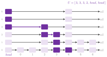
7.9.2 The skip list as a sorted set¶
SkipList realizes the DICTIONARY, and the SSET of Morin (his SkiplistSSet)
by lowerBound( x ), the smallest key not smaller than \(x\) (Morin 2013,
§4.2). Its search, before( k ), follows
the search path of \(k\), dropping a level just before passing \(k\), and returns
the node after the last one met on the level 0 together with \(U\) (Algorithm
7.20). lookup() and contains() compare that
node with \(k\), and lowerBound() returns it. In contrast, the search of Morin
compares \(k\) again with the node that stopped it on the level above whenever
the link it drops to on the next level leads to that same node, i.e., when
\(u.\mathit{next}[ r ] = u.\mathit{next}[ r - 1 ]\) (Morin 2013, exercise
4.8). Ours keeps in \(s\) the last node found
not smaller than \(k\), and drops a level with no comparison when the next link
leads to it, so that \(k\) is compared once with each node.
Algorithm 7.20. The search of SkipList
(Pugh 1990, with Morin 2013, exercise
4.8); \(x.\mathit{next}[ l ]\) is the
successor of \(x\) on the level \(l\), and the head is a node with no key.
Figure 7.21 follows the searches of 2.5 and of 5.5 on the list of Figure 7.20 (Morin 2013, exercise 4.1). The search of 2.5 meets the node 4 on the level 5 and drops with no further comparison on the level 4. On the level 3 it moves to 2, and from there it drops to the level 0, comparing 2.5 only with 3 on the level 2. The search of 5.5 moves to 4 on the level 5, drops along the nil links of 4 down to the level 1 with no comparison, moves to 5, and stops before 6.
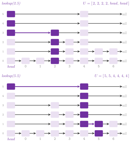
The number of levels of a new node is drawn as the number of trailing 1s of a
random word plus one, i.e., \(\ell\) with probability \(2^{-\ell}\), cut at kMax
= 32. This cut changes nothing unless the list holds far more than \(2^{32}\)
keys (Morin's code counts the trailing 1s of a word of 32 bits, with the same
limit). An insertion of a new key draws \(\ell\), extends the levels in use if
\(\ell > L\) (the new levels start at the head), and splices the node after
\(U[ l ]\) on each of its levels. An insertion of a key already there replaces
its value (Algorithm 7.21). A removal unlinks the
node from each of its levels after before( k ), i.e., after \(U[ l ]\), and
drops the levels left empty. Here the vector \(U\) is the stack of Morin, and
Figure 7.22 shows the insertion of 0.5 with 2
levels and then of 3.5 with 3 levels (Morin 2013, exercise
4.2), Figure
7.23 the removal of 1 and then of 3 (Morin 2013,
exercise 4.3).
Algorithm 7.21. The insertion and the
removal of SkipList (Pugh 1990), the level of a
new node drawn as the number of trailing 1s of a random word plus one.
In C++, SkipList is declared as follows.
// declarations of <ADS/dictionary/SkipList.h>
template< std::totally_ordered K , class V >
class SkipList
{
 public:
 class const_iterator;
 using Key = K;
 using Value = V;
 explicit SkipList( std::uint64_t seed = 1 );
 SkipList( SkipList && other ) noexcept;
 ~SkipList();
 std::optional< V > lookup( const K & k ) const;
 void insert( const K & k , const V & v );
 void remove( const K & k );
 bool contains( const K & k ) const;
 std::size_t size( void ) const;
 bool empty( void ) const;
 int levels( void ) const;
 template< class F >
 void forEach( F && f ) const;
 const_iterator lowerBound( const K & k ) const;
 const K * findKey( const K & k ) const;
 const K * lowerBoundKey( const K & k ) const;
 std::optional< V > fingerLookup( const K & k );
 };
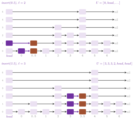
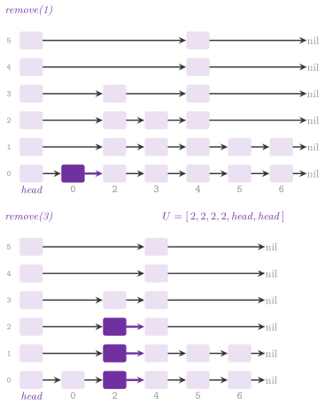
Its contracts check that insert() leaves the key there and remove()
takes it away. They also check the invariant, that each level is sorted and a sublist
of the level below, in \(O( n \log n )\) time at the contract level 3.
forEach() and the forward iterators visit the pairs along the level 0 in
increasing order, and size(), empty() and levels() have the obvious
meaning. The list cannot be copied, since its nodes are linked by pointers,
but it can be moved. Each step of a search, an insertion or a removal takes
constant time, and Lemma 7.23 gives the
theorem of the book.
Theorem 7.6. (Morin 2013, Theorem
4.1.) SkipList realizes the SSET (and
the DICTIONARY), with insert(), remove(), lookup() and
lowerBound() in \(O( \log n )\) expected time each.
An insertion or a removal also changes few links (Morin 2013, exercise 4.6).
Lemma 7.24. An insertion of a key changes 4 links in expectation, and a removal 2.
Proof. An insertion of a node of \(\ell\) levels writes its \(\ell\) links and the \(\ell\) links into it, those of \(U[ 0 ] , \ldots , U[ \ell - 1 ]\); a removal rewrites the \(\ell\) links into the node. The number of levels has \(E[ \ell ] = \sum_{j \ge 0} \Pr[ \ell > j ] = \sum_{j \ge 0} 2^{-j} = 2\). \(\square\)
7.9.3 The analysis¶
We now prove Lemma 7.23, and bound the size and the height of a skip list, following Morin 2013, §4.4; the proofs rest on a simple fact about the tosses of a coin.
Lemma 7.25. Let \(T\) be the number of tosses of a fair coin up to and including the first heads. Then \(E[ T ] = 2\).
Proof. Let \(I_i\) be 1 if the coin is tossed at least \(i\) times and 0 otherwise; \(I_i = 1\) exactly when the first \(i - 1\) tosses are tails, so that \(E[ I_i ] = 2^{-( i - 1 )}\), and \(T = \sum_{i \ge 1} I_i\) gives \(E[ T ] = \sum_{i \ge 1} 2^{-( i - 1 )} = 2\) by the linearity of the expectation. \(\square\)
Lemma 7.26. A skip list of \(n\) keys has \(2 n\) nodes in its lists in expectation, the head excluded, and \(2 n + O( \log n )\) with the head; its expected height is at most \(\log_2 n + 2\).
Proof. A key is in \(L_r\) with probability \(2^{-r}\), and hence \(L_r\) has \(n / 2^r\) keys in expectation and all the lists \(\sum_{r \ge 0} n / 2^r = 2 n\). Let \(I_r\), \(r \ge 1\), be 1 if \(L_r\) is not empty; the height is \(h = \sum_{r \ge 1} I_r\), and \(E[ I_r ] \le \min\{ 1 , E[ | L_r | ] \} = \min\{ 1 , n / 2^r \}\), so that \(E[ h ] \le \lfloor \log_2 n \rfloor + \sum_{r > \lfloor \log_2 n \rfloor} n / 2^r \le \log_2 n + 2\). Finally, the head occurs once per level, \(h + 1\) times. \(\square\)
Proof of Lemma 7.23. Consider the search path backwards, from the last node before \(x\) on the level 0: at each node it goes up if the node has a further level, and left otherwise, and this reverse search path is the search path reversed. On a level \(r\), the steps to the left before going up are those of a coin tossed until it comes up heads (the node has a further level), at most \(E[ T ] - 1 = 1\) in expectation by Lemma 7.25. This bound also holds when the head stops the path earlier. Let \(S_r\) be the number of the steps to the right of the search on the level \(r\), with \(E[ S_r ] \le \min\{ 1 , E[ | L_r | ] \} = \min\{ 1 , n / 2^r \}\), since the path cannot take more steps than \(L_r\) has keys. The length of the path is \(h + \sum_{r \ge 0} S_r\), whose expectation is at most \(E[ h ] + \lfloor \log_2 n \rfloor + 1 + \sum_{r > \lfloor \log_2 n \rfloor} n / 2^r \le E[ h ] + \log_2 n + 3 \le 2 \log_2 n + 5\) by Lemma 7.26. \(\square\)
Theorem 7.7. (Morin 2013, Theorem 4.3.) A skip list of \(n\) keys takes \(O( n )\) expected space, and the expected length of the search path of any key is at most \(2 \log_2 n + O( 1 )\).
This analysis carries over to a promotion with any probability \(p\), \(0 < p < 1\), instead of \(1 / 2\) (Morin 2013, exercise 4.7).
Lemma 7.27. If each key is promoted from a level to the next with probability \(p\), the expected height is \(\log_{1/p} n + O( 1 )\), the expected number of nodes is \(n / ( 1 - p )\), and the expected length of a search path is at most \(\frac{1}{p} \log_{1/p} n + O( 1 )\), least for \(p = 1 / e\).
Proof. A key reaches the level \(j\) with probability \(p^j\); hence, the level \(j\) holds \(n p^j\) keys in expectation, below 1 above \(\log_{1/p} n\), and the nodes are \(\sum_j n p^j = n / ( 1 - p )\). Read backwards, a search path goes up at each node with probability \(p\) and left otherwise. It thus makes \(1 / p\) steps per level in expectation (Lemma 7.25 with a biased coin) over \(\log_{1/p} n\) levels, and the levels above add \(O( 1 )\), as in the proofs above. The factor \(\frac{1}{p \ln( 1 / p )}\) of \(\ln n\) in \(\frac{1}{p} \log_{1/p} n\) has derivative zero where \(\ln( 1 / p ) = 1\), i.e., at \(p = 1 / e\), where the path is \(e \ln n \approx 1.88 \log_2 n\) steps, against \(2 \log_2 n\) for \(p = 1 / 2\). \(\square\)
Yet, the gain of \(p = 1 / e\) is rather small, and the cost of drawing a level with probability \(1 / e\), instead of counting the trailing 1s of a word, does not repay it in our view; the code keeps \(p = 1 / 2\). The saving of the comparisons of Algorithm 7.20 can be counted in the same model (Morin 2013, exercise 4.8).
Lemma 7.28. With the promotion probability \(p\), the search of Algorithm 7.20 compares the key \(( \frac{1}{p} - p ) \log_{1/p} n + O( 1 )\) times in expectation, i.e., \(1.5 \log_2 n + O( 1 )\) for \(p = 1 / 2\), against \(\frac{1}{p} \log_{1/p} n + O( 1 )\) for the search of Morin.
Proof. Morin's search compares the key once per step to the right and once per level to stop, about \(\frac{1}{p}\) times per level by the proof of Lemma 7.27. Ours skips the comparison that stops the level \(l\) when the successor on the level \(l\) of the node where the search stands is the node \(s\) that stopped the level \(l + 1\), i.e., when that successor has a further level. This happens with probability \(p\), independently of the nodes before the key that the search has examined. Hence it saves \(p\) comparisons per level in expectation, \(p \log_{1/p} n + O( 1 )\) in all. \(\square\)
In the test ods_trees.ods-ex4.8.no-redundant-comparisons we count the
comparisons of the searches of a list of 3000 keys and check that no node
is compared twice and that their mean lies between \(1.2 \log_2 n\) and
\(1.8 \log_2 n + 2\). This saving counts when comparing a key costs more than
a word, e.g., for the strings.
7.9.4 Finger search¶
A finger is the sequence of the nodes where a search path goes down, \(U\)
above; it points out the path to a node of \(L_0\) (Morin 2013, exercise
4.10). fingerLookup( k ) keeps the finger
\(F\) of the previous fingerLookup(), \(F[ l ]\) the last node before the
previous key on the level \(l\) (the head counting as \(-\infty\)). It climbs the
finger from the bottom while the node of the level is not before \(k\) or its
successor is, and then goes down from the first one that brackets \(k\),
updating \(F\) (Algorithm 7.22). Note that the
finger stays valid along the levels above the one the search starts from,
whose nodes still bracket the new key, and an insertion or a removal brings it
back to the head (Pugh 1990b).
Algorithm 7.22. The finger search of
SkipList (Pugh 1990b; Morin 2013,
exercise 4.10).
Lemma 7.29. A finger search of a key with \(r\) keys between it and the key of the previous finger search takes \(O( 1 + \log r )\) expected time.
Proof. Let \(x'\) be the previous key, say \(x' < k\) (the other case is symmetric). The finger node \(F[ j ]\), the last node before \(x'\) on the level \(j\), fails to bracket \(k\) only if some node of the level \(j\) has its key in \([ x' , k )\). At most \(r + 1\) keys lie there, each on the level \(j\) with probability \(2^{-j}\), and hence the climb passes the level \(j\) with probability at most \(( r + 1 ) 2^{-j}\), and the level \(l\) where it stops is \(\log_2 ( r + 1 ) + O( 1 )\) in expectation. Then the descent from \(F[ l ]\) goes right only over keys before \(k\) on each level \(j \le l\). Read backwards from its end, it goes up at each node with probability \(1 / 2\) and left otherwise, at most 2 steps per level in expectation by Lemma 7.25, i.e., \(O( l + 1 )\) steps in all. Both parts take \(O( 1 + \log r )\) expected steps. \(\square\)
In the test ods_trees.ods-ex4.10.finger-search we alternate near and
far keys, and check that the finger survives the insertions and the removals
in between.
7.9.5 Widths and the search by rank¶
The width of a link of the level \(r\) is the number of links of \(L_0\) below
it, i.e., the difference of the ranks of its two ends, a link of the level 0
having width 1 (Pugh 1990b; Morin 2013,
§4.3 calls it the length of the edge). If a
search stands at a node of rank \(j\) and follows a link of width \(w\), it
reaches the node of rank \(j + w\). A search by key that sums the widths of the
links it follows thus knows the rank of the node where it stands, and a search
by rank goes along a level while the widths summed stay below the rank.
IndexedSkipList is the skip list of Pugh whose links carry their widths. It
is an SSET that also reaches a key by its rank (select( i ), the get( i )
of Morin 2013, exercise 4.9) and gives the
rank of a key (rank( k ), the number of keys smaller than \(k\)), both in
\(O( \log n )\) expected time; forEach( f ) visits the pairs by increasing
keys. Here the ranks are shifted by one, the head at 0 and the nil at \(n + 1\);
hence, the widths of each level sum to \(n + 1\), the invariant that its
contracts check (Figure 7.24, Algorithm
7.23). Morin gives no code for it, and
SkipListSequence of Chapter 2 is his SkiplistList,
which uses the same widths for a sequence searched by index.
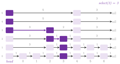
Algorithm 7.23. The search by rank, the
insertion and the removal of IndexedSkipList (Pugh 1990b);
\(x.w[ l ]\) is the width of the link of \(x\) on the level \(l\), \(U[ l ]\) the
last node before \(k\) on the level \(l\) and \(r[ l ]\) its rank, the head of
rank \(-1\) (the ranks of the pseudocode are not shifted, those of the
figures are), and \(y\) the new node of \(\ell\) levels.
The search by key sums the widths along the path, with the saving of the
comparisons of SkipList, and the search by rank needs no comparison of
keys (Algorithm 7.23).
An insertion splits the link that it crosses on each of its levels, and adds 1 to the width of those that pass over it. A removal does the reverse, on each level of its node replacing the link that reaches it by the one that leaves it, their widths summed less 1, and subtracting 1 from the links that pass over it:
Below are the declarations of IndexedSkipList, followed by an example of use.
// declarations of <ADS/dictionary/IndexedSkipList.h>
template< std::totally_ordered K , class V >
class IndexedSkipList
{
 public:
 class const_iterator;
 using Key = K;
 using Value = V;
 explicit IndexedSkipList( std::uint64_t seed = 1 );
 IndexedSkipList( IndexedSkipList && other ) noexcept;
 ~IndexedSkipList();
 std::optional< V > lookup( const K & k ) const;
 void insert( const K & k , const V & v );
 void remove( const K & k );
 bool contains( const K & k ) const;
 std::size_t size( void ) const;
 bool empty( void ) const;
 std::size_t rank( const K & k ) const;
 template< class F >
 void forEach( F && f ) const;
 const_iterator lowerBound( const K & k ) const;
 const K * findKey( const K & k ) const;
 const K * lowerBoundKey( const K & k ) const;
 const_iterator select( std::size_t i ) const;
 };
ADS::IndexedSkipList< int , char > S;
for( int k : { 30 , 10 , 20 } )
 S.insert( k , 'a' + k / 10 );
const std::size_t r = S.rank( 20 );     // 1
const int * y = S.lowerBoundKey( 15 );  // *y == 20
Lemma 7.30. The insertion and the removal of
IndexedSkipList keep the width of each link equal to the difference of the
ranks of its ends; hence the widths of each level sum to \(n + 1\). With these
widths, select( i ) and rank( k ) take \(O( \log n )\) expected time.
Proof. Let the new node \(y\) take the shifted rank \(i\), and let the link of
\(U[ l ]\), of shifted rank \(r[ l ]\), have the width \(w\) before the insertion,
its end at \(r[ l ] + w\). On a level of \(y\), the link of \(U[ l ]\) now ends at
\(y\), with width \(i - r[ l ]\), and the link of \(y\) ends where the old link did,
whose rank grew by one with the new key, i.e., at \(r[ l ] + w + 1\), with width
\(r[ l ] + w + 1 - i\). On a level above \(y\), the link of \(U[ l ]\) passes over
\(y\) and its end moves up by one rank, so that its width grows by 1. No other
link has an end before \(y\) and the other after it on its level, and the widths
of the other links do not change. A removal is the same computation backwards;
the links of the head of the levels not in use pass over each key and grow and
shrink with \(n\). Finally, rank( k ) follows the search path of \(k\), adding
the widths of the links it follows, and select( i ) goes right on a level
exactly over the nodes of rank at most \(i\), i.e., of key at most the key \(x_i\)
of rank \(i\); it thus follows the search path of a value between \(x_i\) and the
key after it. Both paths have \(O( \log n )\) expected length by Lemma
7.23, which holds for any value searched, and each
step costs \(O( 1 )\). \(\square\)
Figure 7.25 applies the two operations to the
list of Figure 7.24, i.e., the removal of the key
of rank 2 (Morin 2013, exercise 4.4, his
remove( 2 )) and the insertion at the rank 3 of a node of 5 levels (Morin
2013, exercise 4.5, his add( 3 , x ) with
a height of 4, the splice of his Figures 4.6 and 4.7). In IndexedSkipList
the latter is the insertion of a key between 2 and 3, here 2.5, and
SkipListSequence makes the same changes by index. It also has
truncate( i ) and absorb( l ) (Morin 2013, exercises 4.11 and
4.12), described in Chapter
2 with the theorem of the SkiplistList (Morin 2013,
Theorem 4.2).
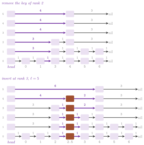
7.9.6 Applications and the comparison with the trees¶
Each substring of a text is a prefix of one of its suffixes. Hence, an
SSET of the suffixes, each a view of the text from its first character
(i.e., an integer), finds a substring \(q\) as the first suffix not smaller
than \(q\), when \(q\) is a prefix of it (Morin 2013, exercise
4.14). Each keystroke costs \(O( | q |
\log n )\) expected time, the comparisons of a search being of \(| q |\)
characters at most, and the test ods_trees.ods-ex4.14.substring-search
runs such a search after each character typed. A suffix array (Manber and
Myers 1993;
§15.5) holds the same suffixes in \(n\) words with
no links, while the SSET allows changes of the text. A space-efficient
SSET of Morin 2013, exercise 4.13, which
stores the keys in blocks of a space-efficient list and the blocks in a
skip list, is SpaceEfficientSortedSet of ADS/set (Chapter
10).
A skip list whose links point only right on each level, and down from each node to the same node on the level below, is a binary tree once the right links into a node below its top level are dropped (that node is reached from above). The right link and the down link are the two children of a pair (node, level), and the search follows a path of it as in a binary search tree (Morin 2013, exercise 4.15, Figure 7.26; cf. Chapter 8). It uses its links better, however: a binary search tree of \(n\) nodes has \(2 n\) links of which \(n + 1\) are nil, while a skip list has \(2 n\) links in expectation (Lemma 7.26) of which only those at the end of each level, \(O( \log n )\), are nil.
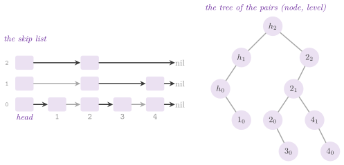
7.10 Tries of strings¶
A trie (Fredkin 1960) stands for a set of strings by a tree whose node at depth \(d\) is a prefix of \(d\) characters, the children of a node indexed by the next character and the nodes that end a key marked. A search reads one node per character, in time that depends on the length of the key and not on the number of the keys; also, the keys with a given prefix are the marked nodes below the node of the prefix, in lexicographic order (Knuth 1998, §6.3). Headers of this section go from the trie of the textbooks to the compact, the blind, the adaptive and the succinct tries. The search by prefix on sorted arrays and the front coding are in §15.6.
7.10.1 The trie and the compact trie¶
Trie keeps the children of a node in a sorted map (std::map by character),
and hence a search, an insertion and a removal take \(O( | k | \log \sigma )\)
time for a key of \(| k |\) characters on an alphabet of \(\sigma\) (Algorithm
7.24). An insertion makes the nodes missing on the
path of \(k\), and a removal removes, bottom up, the nodes of its path left with
no value and no child. keysWithPrefix( p ) gives the keys below the node of
\(p\) in increasing order, and nodes() the number of nodes, the root included.
Its space is \(O( N )\) nodes for keys of total length \(N\), a node per character
not shared with another key.
Algorithm 7.24. The lookup of Trie
(Fredkin 1960; Knuth 1998,
§6.3) and the insertion of
RadixTree, \(\lambda( y )\) being the label of the edge into \(y\).
We declare Trie and RadixTree as follows, followed by an example of use.
// declarations of <ADS/dictionary/Trie.h>
template< class V >
class Trie
{
 public:
 using Key = std::string;
 using Value = V;
 std::optional< V > lookup( std::string_view k ) const;
 void insert( std::string_view k , const V & v );
 void remove( std::string_view k );
 bool contains( std::string_view k ) const;
 std::size_t size( void ) const;
 std::vector< std::string > keysWithPrefix( std::string_view p ) const;
 std::size_t nodes( void ) const;
 using const_iterator = detail::TrieIterator< Node , V , false >;
 };
template< class V >
class RadixTree
{
 public:
 using Key = std::string;
 using Value = V;
 std::optional< V > lookup( std::string_view k ) const;
 void insert( std::string_view k , const V & v );
 void remove( std::string_view k );
 bool contains( std::string_view k ) const;
 std::size_t size( void ) const;
 std::vector< std::string > keysWithPrefix( std::string_view p ) const;
 std::size_t nodes( void ) const;
 using const_iterator = detail::TrieIterator< Node , V , true >;
 };
ADS::Trie< int > T;
T.insert( "car" , 1 );
T.insert( "cart" , 2 );
T.insert( "dog" , 3 );
const auto w = T.keysWithPrefix( "car" );  // { "car" , "cart" }
RadixTree is the compact trie (the Patricia of Morrison
1968, on characters rather than on
bits). Each chain of nodes with a single child and no mark is merged into
one edge labeled by a string, and the children of a node are indexed by the
first characters of their labels, which are distinct. An insertion splits
an edge where the new key departs from its label, and a removal merges back
a node left with a single child and no value (compress()). Hence, the
invariant (no node but the root has a single child and no mark, checked by
compact()) holds after each operation (Figure
7.27). Both tries are DICTIONARIES whose keys
are strings, and their iterators (TrieIterator) visit the keys in
lexicographic order by a visit in depth with a stack of the children still
to see. They rebuild the key along the path, a character per edge or the
label of the child.
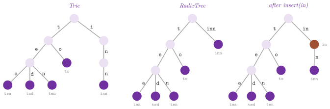
Lemma 7.31. A compact trie of \(n\) keys has at most \(2 n\) nodes besides the root, however long the keys are.
Proof. Marked nodes are \(n\). An unmarked node other than the root has at least two children, and the leaves are all marked. In a tree the children of all the nodes are the nodes less the root. Hence the internal nodes \(u\) satisfy \(\sum_u ( c( u ) - 1 ) = \lambda - 1\), where \(c( u )\) is the number of the children of \(u\) and \(\lambda\) that of the leaves. Each term is at least 0, and at least 1 for an unmarked node other than the root; there are thus at most \(\lambda - 1 \le n - 1\) such nodes. \(\square\)
7.10.2 The blind search of the Patricia trie¶
PatriciaTrie is the compact trie of a sorted dictionary \(D\) of \(n\)
strings stripped of the labels, each edge keeping only its first character
(the branching one) and each node the length of the prefix it stands for.
It thus takes \(O( n )\) space whatever the length of the strings, which are
stored apart, e.g., on disk (Ferragina and Grossi
1999; Ferragina 2023, chapter
9). A string that is a prefix of
another ends with a character smaller than all the others, and therefore
the leaf of a string \(s\) has length \(| s | + 1\). The blind search of a
pattern \(P\) of \(p\) characters finds its lexicographic position, the number
of the strings smaller than \(P\), reading a single string. It works in three
stages (Algorithm 7.25, Figure
7.28). First, it goes down from the root
comparing only the branching characters with the characters of \(P\) at the
lengths of the nodes, possibly skipping characters that do not match, until
a leaf or a node with no edge for \(P\), and takes a leaf below it
(blindLeaf()). It computes the longest common prefix \(\ell\) of \(P\) and of
the string \(s\) of that leaf. Finally, it finds on the path the edge \(( u ,
v )\) where \(\ell\) falls, \(| u | \le \ell < | v |\). Then the position of \(P\)
is among the children of \(u\), by the character \(P[ \ell ]\), if \(\ell = | u
|\), and otherwise just before or just after the strings below \(v\), by the
comparison of \(P[ \ell ]\) with \(s[ \ell ]\).
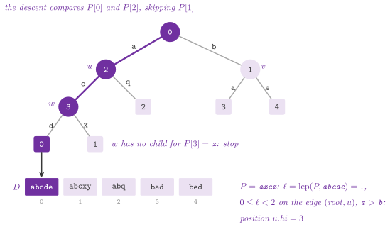
Algorithm 7.25. The blind search and the
construction of PatriciaTrie (Ferragina 2023,
chapter 9); \(| x |\) is the depth of
the node \(x\), \(x.\mathit{lo}\) and \(x.\mathit{hi}\) the range of its strings,
\(P\) followed by a character smaller than all the others, and \(\ell_i\) the
longest common prefix of \(D[ i - 1 ]\) and \(D[ i ]\).
In C++, PatriciaTrie is declared as follows.
// declarations of <ADS/dictionary/PatriciaTrie.h>
class PatriciaTrie
{
 public:
 explicit PatriciaTrie( std::vector< std::string > D );
 std::size_t lexicographicPosition( std::string_view P ) const;
 std::size_t prefixEnd( std::string_view P ) const;
 std::pair< std::size_t ,
            std::size_t > prefixRange( std::string_view P ) const;
 std::size_t blindLeaf( std::string_view P ) const;
 bool contains( std::string_view P ) const;
 std::size_t size( void ) const;
 std::size_t nodes( void ) const;
 const std::string & string( std::size_t i ) const;
 std::vector< std::pair< std::size_t , int > > shape( void ) const;
 using const_iterator = std::vector< std::string >::const_iterator;
 };
Lemma 7.32. The blind search returns the number of the strings of \(D\) smaller than \(P\).
Proof. Let \(\ell'\) be the longest prefix of \(P\) shared by some string of \(D\). The first \(\ell'\) characters of \(P\) drive the descent along the path of that prefix, since the branching characters met at depths below \(\ell'\) are those of \(P\), up to the node of depth at most \(\ell'\) where the path of \(P\) parts from the trie. Each leaf below that node shares with \(P\) its first \(\ell'\) characters, and therefore the leaf read has \(\ell = \ell'\). The node \(u\) at depth \(| u | \le \ell < | v |\) is then the deepest node whose prefix is a prefix of \(P\). If \(\ell = | u |\), \(P\) leaves the trie at \(u\), and the strings smaller than \(P\) are those before \(u\) and those below the children of \(u\) with a branching character smaller than \(P[ \ell ]\). If \(\ell < | v |\), all the strings below \(v\) share the first \(\ell\) characters with \(P\) and have \(s[ \ell ]\) at the place \(\ell\), and hence they all precede \(P\) if \(P[ \ell ] > s[ \ell ]\) and all follow it otherwise. \(\square\)
Both traversals take \(O( p \log \sigma )\) time with the edges of a node in a
sorted array, and touch no string. The comparison of the third stage reads one
string, i.e., \(O( p / B )\) transfers of blocks of \(B\) characters, against the
\(O( p )\) of the compact trie, which reads a label per edge, and the
\(O( ( p / B ) \log n )\) of the binary search over the strings
(§15.6.1). The positions of \(P\) and of \(P\#\), \(\#\)
a character larger than all the others, give the range of the strings prefixed
by \(P\) (lexicographicPosition(), prefixEnd() and prefixRange()). This
trie is built from the sorted strings and the longest common prefixes of
adjacent ones in \(O( N )\) time with a stack of the nodes of the rightmost
path, \(N\) the characters of the strings. contains(), size(), nodes(),
string( i ) and shape() (the length of each node and its branching
character, in preorder) complete the interface. Its invariant is that each
node but the root has at least two children, whose characters increase and
whose strings are consecutive, and the test pearls_hashing.patricia replays
the example of Ferragina 2023, Figures 9.7 and
9.8.
TwoLevelDictionary puts a Patricia trie over the front coding of the sorted
strings with anchors (FrontCodedDictionary of ADS/string/FrontCoding.h,
§15.6.2). Anchors are the strings stored whole, one
every \(b\) (the bucketing) or as the locality-preserving coding decides, and
the trie holds the anchors alone (Figure 7.29). A
search by prefix is the blind search of the pattern among the anchors, which
reads one anchor, and the scan of the one bucket where the pattern falls,
decoded on the fly (Algorithm 7.26). With the
trie in memory and the coding on disk, it costs \(O( p / B + | s | / B )\)
transfers of blocks plus the bucket, \(s\) being the string read by the blind
search, in \(O( n_a )\) words of memory for \(n_a\) anchors, and
\(( 1 + \epsilon ) \mathrm{FC}( D )\) characters on disk with the
locality-preserving coding (Ferragina 2023, chapter
9). The binary search on the anchors
costs \(O( ( p / B ) \log n_a )\) transfers instead. When even the trie does not
fit in memory, the string B-tree of Ferragina and Grossi
1999 splits it into Patricia tries of a
block each, linked as a B-tree, for
\(O( ( p + N_{\mathit{occ}} ) / B + \log_B n )\) transfers; also, the
cache-oblivious version of Bender et
al. 2006 drops \(B\) from the code. upper()
and lower() give the two levels, access( i ) decodes the string \(i\) from
its bucket, and anchorsOf() extracts the anchors of a coding.
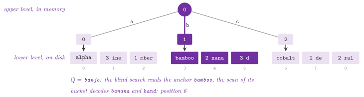
Algorithm 7.26. The search of
TwoLevelDictionary (Ferragina 2023, chapter
9), the trie \(T\) in memory and the
buckets of the coding on disk.
Below are the declarations of TwoLevelDictionary.
// declarations of <ADS/dictionary/TwoLevelDictionary.h>
class TwoLevelDictionary
{
 public:
 explicit TwoLevelDictionary( FrontCodedDictionary F );
 std::size_t lexicographicPosition( std::string_view Q ) const;
 std::size_t prefixEnd( std::string_view P ) const;
 std::pair< std::size_t ,
            std::size_t > prefixRange( std::string_view P ) const;
 std::string access( std::size_t i ) const;
 std::size_t size( void ) const;
 const PatriciaTrie & upper( void ) const;
 const FrontCodedDictionary & lower( void ) const;
 using const_iterator = FrontCodedDictionary::const_iterator;
 };
7.10.3 The adaptive radix tree¶
AdaptiveRadixTree is the adaptive radix tree of Leis et al.
2013 on strings, the engineered ordered
DICTIONARY of the library whose keys are strings, which the benchmark of
the tries compares with the HAT-trie of tsl, with libart and with the
B-trees of strings. A node at depth \(d\) stands for the prefixes of \(d\)
bytes of its keys and branches on their byte \(d\), and it adapts its layout
to the number of its children, and hence a node is never much larger than
its pointers (Figure 7.30). Layouts Node4 and Node16 keep up to 4 and 16 bytes sorted beside the pointers
to the children of the same places; a Node16 is searched by one
comparison of the vectors of Highway (SSE2, NEON), the 16 bytes against the byte of
the key at once. Node48 keeps an index of 256 bytes, the place of the
child of each byte among its 48 pointers (0 for none); Node256 keeps the
256 pointers, the byte of the key being the place. A node grows to the next
layout when it is full and shrinks to the previous one when it holds at
most 3 children (a Node16), 12 (a Node48) or 37 (a Node256), i.e.,
when the smaller layout would keep about a quarter of its places free (1
of 4, 4 of 16, 11 of 48). This is a slack against the repeated changes of
layout of an insertion and a removal at the threshold.
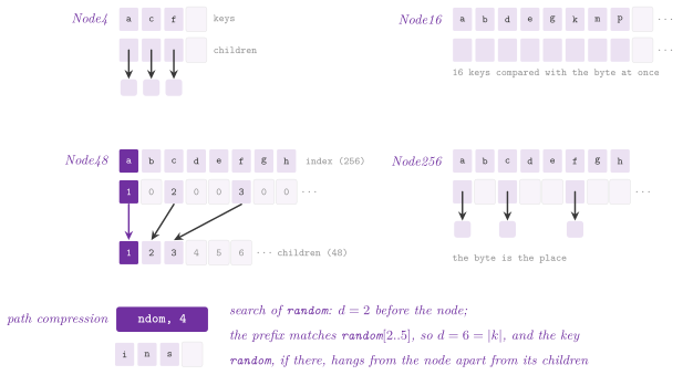
A chain of nodes with a single child is compressed into the prefix of the
first node that branches (the path compression). The prefix is the length
of the chain and its first 8 bytes, and a search skips the bytes past 8
(the optimistic compression of the paper, the hybrid of its section III.E)
and compares the full key at the leaf, where each search ends (Algorithm
7.27). A leaf holds the whole key, in one
allocation with its value, and a pointer to a child is a leaf if its lowest
bit is set (isLeaf(), asLeaf(), tag()). A key that ends at a node,
a prefix of all the keys below it, hangs from the node apart from the
children, so that any string, null bytes included, can be a key. An
insertion first descends as a search: if no prefix on the way was longer
than its 8 bytes, the way is the one of the key, and the key goes where the
search stopped, in one pass. Otherwise the search ends at a leaf \(l\) below
the last node that the key reaches. A second pass then goes down again to
the node or the leaf whose prefix parts from the key at the first byte
where the key and \(l\) differ, the full prefixes of the nodes on the way
being those of \(l\). A removal shrinks the node of its key below a quarter
of its places and merges a node left with a single child into its prefix.
Algorithm 7.27. The search and the insertion
of AdaptiveRadixTree (Leis et al.
2013); \(d\) is the number of the bytes of
\(k\) consumed, a prefix being compared on its first 8 bytes only and the
leaf on the whole key.
We declare AdaptiveRadixTree as follows.
// declarations of <ADS/dictionary/AdaptiveRadixTree.h>
template< class V >
class AdaptiveRadixTree
{
 public:
 using Key = std::string;
 using Value = V;
 AdaptiveRadixTree( void ) = default;
 AdaptiveRadixTree( const AdaptiveRadixTree & o );
 AdaptiveRadixTree( AdaptiveRadixTree && o ) noexcept;
 ~AdaptiveRadixTree();
 std::optional< V > lookup( std::string_view k ) const;
 const V * find( std::string_view k ) const;
 V * find( std::string_view k );
 bool insert( std::string_view k , const V & v );
 bool remove( std::string_view k );
 bool contains( std::string_view k ) const;
 std::size_t size( void ) const;
 bool empty( void ) const;
 void clear( void );
 void swap( AdaptiveRadixTree & o ) noexcept;
 template< class F >
 void forEach( F && f ) const;
 template< class F >
 void forPrefix( std::string_view p , F && f ) const;
 std::vector< std::string > keysWithPrefix( std::string_view p ) const;
 class const_iterator;
 };
Lemma 7.33. An adaptive radix tree of \(n\) keys has at most \(n - 1\) internal nodes and \(n\) leaves, and a search, an insertion and a removal of a key of \(k\) bytes take \(O( k )\) time, whatever \(n\).
Proof. Each internal node, the root included, has at least two things below it among its children and its own key, since a removal merges a node with one child and no key into the prefix of its child, and replaces a node with no child by its key. Let \(I\) be the internal nodes, \(c( u )\) the children of \(u\) and \(t( u ) \in \{ 0 , 1 \}\) its own key; the children of all the nodes are the nodes less the root, i.e., \(I + \lambda - 1\) for \(\lambda\) leaves, and \(n = \lambda + \sum_u t( u )\). Hence \(2 I \le \sum_u ( c( u ) + t( u ) ) = I - 1 + n\), i.e., \(I \le n - 1\). A search consumes at least one byte of the key at each node, the byte that selects the child, and spends \(O( 1 )\) time per node whatever its layout, while the comparison of the prefixes and of the leaf reads each byte of the key \(O( 1 )\) times. An insertion and a removal make at most two passes and change \(O( 1 )\) nodes. \(\square\)
A leaf of a key of \(k\) bytes and a value of 8 takes \(\lceil ( 16 + k ) / 16
\rceil\) slots of 16 bytes. A search prefetches the lines of the next node
that it reads for its byte, whatever the layout, while the first line is on
its way (ahead()), and the visits prefetch the children of a Node4 or a
Node16 (children()). Its iterators visit the pairs by increasing keys,
a key before the longer ones that begin with it and the children of a node
by their bytes, as a string_view on the key of the leaf and a constant
reference to its value. They keep a stack of the nodes on the way.
forEach() and forPrefix() visit all the pairs, and those whose key
begins with a prefix, by a recursion with no stack, keysWithPrefix()
returns those keys, and find() gives a value to change in place, and
clear() frees all the nodes and the leaves. An insertion or a removal
invalidates the iterators. Its internal nodes come from pools on huge pages
(Chapter 5), the leaves from slabs of 16 to 512 bytes
in steps of 16 (Slab, after the slab allocator of Bonwick
1994), each size with the list of its
free slots, cut from blocks that double up to 2 MB. Hence, a leaf costs no
call to the allocator. Its invariant, checked at the contract level 3 on
the trees of up to 2048 keys, requires that the keys of the leaves extend
the paths that lead to them. It also requires that each node but the root
branches or ends a key, and that the bytes of a node are sorted and its
layout the one of its count. Finally, the leaves must be size().
7.10.4 The Patricia trie in succinct space¶
SuccinctPatriciaTrie codes the shape of the compact trie of a static
dictionary of \(n\) strings by the degrees of its nodes in depth (DFUDS) of
Benoit et al. 2005, with the first
character of each edge in a byte and the rest of its label in a string
apart. It maps a string to its rank in the lexicographic order. The \(N\)
nodes of the compact trie, at most \(2 n\) by Lemma
7.31, are visited in depth, the children of a
node by their first characters. The node of \(d\) children is written as \(d\)
open parentheses and a closed one, after an open parenthesis that balances
the whole. This takes \(2 N\) bits, in which the node of rank \(v\) in the
visit begins after the \(v\)-th closed parenthesis (Figure
7.31). With the matching of the parentheses
(BalancedParentheses.h, Chapter 22), the \(i\)-th
child of the node at the place \(p\), of degree \(d\), begins after the closed
parenthesis that matches the open one at \(p + d - 1 - i\). Indeed, the last
open parenthesis of the node is matched by the closed one that ends it,
right after which the first child begins. The first characters of the
children of a node are consecutive, in the order of the open parentheses,
so that the child of a character is found by a binary search on at most
\(\sigma\) bytes.
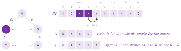
Lemma 7.34. The parentheses of the subtree of the node at the place \(p\) are those from \(p\) to the first place \(e\) whose excess (the open parentheses less the closed ones up to it) is one less than at \(p - 1\), and the nodes of the subtree are the consecutive ranks from that of the node at \(p\) to the number of the closed parentheses up to \(e\).
Proof. An open parenthesis followed by the code of a subtree is the code of that subtree as a tree of its own, which is balanced: its excess comes back to the level before the open parenthesis only at its end. The code of the subtree alone, without that parenthesis, thus goes one level below the excess at \(p - 1\) for the first time at its last parenthesis. Also, the visit in depth writes the nodes of the subtree one after the other, each ending with a closed parenthesis. \(\square\)
Hence, with a vector of bits \(T\) that marks the nodes where a string ends, the
rank of a string among the marks is its rank in the lexicographic order (a
node comes before its subtree, which holds the strings it prefixes, and the
subtrees follow the order of their first characters). Also, the strings with a
prefix \(P\) are the marks of the subtree where the walk of \(P\) ends, a range of
ranks found by one forward search (Algorithm
7.28). A lookup of \(Q\) walks down \(O( | Q | )\)
nodes, each in \(O( \log \sigma )\) time besides a rank, a select of Elias and
Fano for the rest of its label and, but for the first child, a findClose(),
and contains( Q ) is a lookup that found \(Q\). In turn,
lexicographicPosition( Q ), the number of strings smaller than \(Q\), walks as
the lookup up to the first mismatch and takes the rank of the end of a subtree
there. access( i ) walks up from the node of the string of rank \(i\) by
findOpen(), prepending the labels. Its space is \(2 N + o( N )\) bits for the
parentheses with their range min-max tree, \(8 ( N - 1 )\) for the first
characters, \(2 N + o( N )\) for the marks of the ends and of the nodes with a
rest, and the rests of the labels, one after the other, with their places by
Elias and Fano. Finally, bytes() reports the total. In contrast, the
path-decomposed tries of Grossi and Ottaviano
2015 and the dictionaries of
Martínez-Prieto et al. 2016
compress the labels as well, by Re-Pair or by the codes of Hu and Tucker,
which is not done here. Instead, the front coding with buckets of
RearCoding.h (§15.6.3) may be smaller still on
strings with long shared prefixes. Its audit of the construction checks that
access() and lookup() invert each other, and the test
engineered_strings.string-dictionaries exercises both.
Algorithm 7.28. The construction, the
lookup, the access and the range of a prefix of SuccinctPatriciaTrie
(Benoit et al. 2005); a node is the
range \([ l , r )\) of the strings below it with the depth \(h\) of its end,
\(\lambda( v )\) is the rest of the label of the node \(v\), \(p_v\) and \(d_v\) its
place and its degree, and \(T\) the marks of the nodes where a string ends.
In C++, SuccinctPatriciaTrie is declared as follows.
// declarations of <ADS/dictionary/SuccinctPatriciaTrie.h>
class SuccinctPatriciaTrie
{
 public:
 SuccinctPatriciaTrie( void );
 explicit SuccinctPatriciaTrie( const std::vector< std::string > & D );
 std::size_t size( void ) const;
 bool empty( void ) const;
 std::size_t nodes( void ) const;
 std::size_t lookup( std::string_view Q ) const;
 bool contains( std::string_view Q ) const;
 std::string access( std::size_t i ) const;
 std::size_t lexicographicPosition( std::string_view Q ) const;
 std::pair< std::size_t ,
            std::size_t > prefixRange( std::string_view P ) const;
 std::size_t bytes( void ) const;
 };
7.11 Structures for integers¶
We return to the SORTED SET, now with keys that are integers of \(w\) bits,
\(x \in \{ 0 , \ldots , 2^w - 1 \}\), each with a value (Morin 2013, chapter
13). Three structures follow, each built on
the previous one: the binary trie performs the three operations in \(O( w )\)
time, which is not much, since a set of \(n \le 2^w\) keys has \(\log n \le w\)
and each comparison-based SSET of the book is at least as fast. The x-fast
trie brings lowerBound() to \(O( \log w )\) expected time by hashing, but its
updates still take \(O( w )\) and its space is \(O( n w )\). The y-fast trie
stores in an x-fast trie only a sample of about one key in \(w\), and the others
in treaps, which brings the updates to \(O( \log w )\) and the space to
\(O( n )\). Our headers also have the simplified tries of the exercises of the
book and its extension to strings. In all of them lowerBound( x ) is the
find( x ) of the SSET of the book, find( x ) the search of \(x\) itself (the
find( x ) of his USET), and the keys are below \(2^w\), a precondition of each
operation. Its parameter W is the width \(w\), between 1 and the bits of the
type of the keys (the concept TrieWidth). Helpers triePrefix(),
trieBit() and trieKey() of the namespace detail give the prefix of \(i\)
bits \(\lfloor x / 2^{w - i} \rfloor\), the bit \(i\) counted from the most
significant one, and whether \(x < 2^w\).
7.11.1 The binary trie¶
BinaryTrie encodes a set of integers of \(w\) bits in a binary tree whose
leaves are all at depth \(w\). Each integer is the path from the root to a
leaf that turns to the child 0 at the depth \(i\) if the bit \(i\) of the key,
counted from the most significant one, is 0, and to the child 1 otherwise
(Morin 2013, §13.1, after
Fredkin 1960). A node at depth \(i\)
thus stands for a prefix of \(i\) bits. The two children of a node serve
twice: the leaves have no children, and they use the two pointers as the
links of a doubly linked list of the keys in increasing order, with a
dummy node before the first and after the last. Each internal node with
one child also keeps a jump pointer, to the smallest leaf below it if its
child 0 is missing, and to the largest if its child 1 is missing
(Figure 7.32).
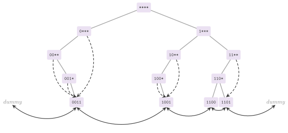
A search of \(x\) follows its path down to the deepest node \(u\) of the path
(deepest()), at depth \(i\). If \(i = w\), \(u\) is the leaf of \(x\); otherwise
the child of \(u\) for the bit \(i\) of \(x\), \(c\), is missing, and the other
child is there. Hence, all the keys below \(u\) are larger than \(x\) if \(c =
0\), and smaller if \(c = 1\). The jump pointer of \(u\) leads to the smallest
of them, which is the successor of \(x\), in the first case, and to the
largest of them, whose next in the list is the successor, in the second
case (Algorithm 7.29, Figure
7.33). Its time is that of the walk down, \(O( w
)\).
Algorithm 7.29. The successor, the
insertion and the removal of BinaryTrie (Morin 2013,
§13.1); \(u\) is the deepest node of the
path of \(x\), at depth \(i\), \(c\) the bit \(i\) of \(x\), and \(\ell\) the leaf of
\(x\).
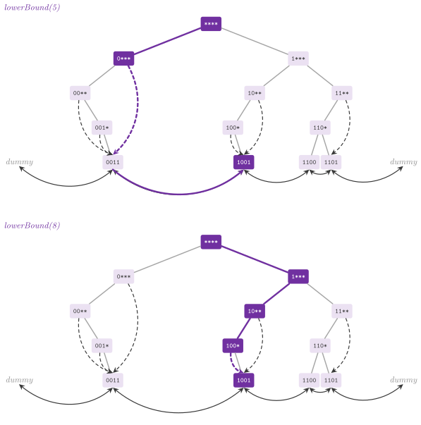
An insertion has more to do. It follows the path of \(x\) down to the deepest node \(u\); it creates the rest of the path, down to a new leaf of \(x\). It links the leaf in the list after its predecessor, which the jump pointer of \(u\) gives as in the search. Finally, it walks back up the path, setting to the new leaf the jump pointer of each ancestor whose child 0 is missing and whose smallest leaf is now \(x\), or whose child 1 is missing and whose largest leaf is now \(x\) (Figure 7.34). A removal undoes it. It unlinks the leaf of \(x\) from the list, removes the nodes of the path of \(x\) from the leaf up while they are left with no child. Then it walks up from the lowest node left to the root, redirecting to the next or to the previous leaf the jump pointers that pointed to the leaf of \(x\) (Figure 7.35). Each of the two walks takes \(O( w )\) time.
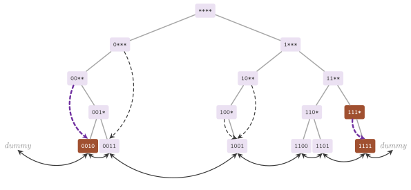
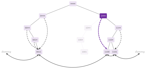
Theorem 7.8. (Morin 2013, Theorem
13.1.) BinaryTrie realizes the SSET of
the integers of \(w\) bits, with insert(), remove() and lowerBound()
in \(O( w )\) time each, in \(O( n w )\) space: the trie has at most
\(n w + 1\) nodes.
Against the code of the book, the nodes come from an ObjectPool (Chapter
5) instead of one call to the allocator each, and those
made one after another lie next to each other. Hence, the \(w\) nodes of a new
path seldom cost an allocation and the walk from the root misses the cache
less. Also, the keys have any width up to 64 bits, where the book fixes
\(w = 32\); and remove() reads the links of the leaf before it frees it, while
the code of the book reads them from the freed leaf. A class template,
detail::JumpTrie, holds the code that BinaryTrie and the x-fast trie
share, and adds find(), lookup(), contains(), min(), max(),
clear(), size(), empty(), nodes() and the bidirectional iterators
along the list (seek( x ) returns the iterator on the successor of \(x\)). Its
invariant (the depth of the leaves, the order of the list, the jump pointers
and, for the x-fast trie, the tables of the prefixes) is checked in \(O( n w )\)
time at the contract level 3 while \(n \le 256\), and at the leaf of the
operation beyond (consistent()).
SimpleBinaryTrie is the trie of Morin 2013, exercise
13.1, with neither the list nor the jump
pointers, its internal nodes being two pointers each and its leaves also a
key and a value. A search that falls off the trie keeps, on its walk down,
the child 1 of the deepest node where the path of \(x\) goes to the child 0
while the child 1 is there, the root \(a\) of the nearest larger keys. It then
returns the leftmost leaf below \(a\), \(O( w )\) more steps (Algorithm
7.30, Figure
7.36). An insertion adds the missing nodes of
its path, a removal removes the nodes of its path left with no child, both
in \(O( w )\) time, and forEach() visits the pairs by increasing keys. It
takes less memory than BinaryTrie, at the price of the walk down to the
leftmost leaf.
Algorithm 7.30. The successor in
SimpleBinaryTrie (Morin 2013, exercise
13.1).
Below are the declarations of BinaryTrie and SimpleBinaryTrie.
// declarations of <ADS/dictionary/BinaryTrie.h>
template< std::unsigned_integral U , class V = std::monostate ,
          int W = std::numeric_limits< U >::digits >
 requires TrieWidth< U , W >
class BinaryTrie : public detail::JumpTrie< U , V , W , false >
{
 public:
 using detail::JumpTrie< U , V , W , false >::JumpTrie;
 class const_iterator;
 using Key = U;
 using Item = U;
 using Value = V;
 const U * lowerBound( U x ) const;
 const U * find( U x ) const;
 std::optional< V > lookup( U x ) const;
 bool contains( U x ) const;
 bool insert( U x , const V & v = V() );
 bool remove( U x );
 std::size_t size( void ) const;
 bool empty( void ) const;
 std::size_t nodes( void ) const;
 std::optional< U > min( void ) const;
 std::optional< U > max( void ) const;
 void clear( void );
 const_iterator seek( U x ) const;
 };
template< std::unsigned_integral U , class V = std::monostate ,
          int W = std::numeric_limits< U >::digits >
 requires TrieWidth< U , W >
class SimpleBinaryTrie
{
 public:
 using Key = U;
 using Item = U;
 using Value = V;
 SimpleBinaryTrie( void ) = default;
 SimpleBinaryTrie( SimpleBinaryTrie && o ) noexcept;
 ~SimpleBinaryTrie();
 const U * lowerBound( U x ) const;
 const U * find( U x ) const;
 std::optional< V > lookup( U x ) const;
 bool contains( U x ) const;
 bool insert( U x , const V & v = V() );
 bool remove( U x );
 std::size_t size( void ) const;
 bool empty( void ) const;
 std::size_t nodes( void ) const;
 template< class F >
 void forEach( F && f ) const;
 };
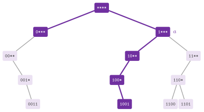
7.11.2 The x-fast trie¶
The search of the binary trie is almost over once it reaches the deepest node
\(u\) of the path of \(x\), and XFastTrie finds \(u\) by a binary search on the
depth instead of a walk (Morin 2013, §13.2,
after Willard 1983). It is a BinaryTrie
with, for each depth \(i = 1 , \ldots , w\), a hash table \(t[ i ]\) from the
prefixes of \(i\) bits to their nodes (TrieTables, and node( p , i ) the
lookup of a prefix). The node \(u\) is at depth \(i\) or below exactly when the
prefix of \(i\) bits of \(x\) is in \(t[ i ]\) (Figure
7.37).
Lemma 7.35. If the prefix of \(i\) bits of \(x\) is the prefix of some key, so is its prefix of \(j\) bits for each \(j < i\). Hence the depth \(\ell\) of the deepest node of the path of \(x\) is found by a binary search on \([ 0 , w ]\), with \(\lceil \log_2 ( w + 1 ) \rceil\) lookups in the tables, and the successor of \(x\) is the smallest key with the prefix of depth \(\ell\) if the bit \(\ell\) of \(x\) is 0, and the key after the largest one with that prefix otherwise.
Proof. A prefix of a prefix of a key is a prefix of the key, which gives the monotonicity on which the binary search rests, keeping a depth whose prefix is there and one whose prefix is not (the root, at depth 0, is always there). The node of the prefix of depth \(\ell\) has no child on the side of the bit \(\ell\) of \(x\), and hence all its keys are on the other side, all larger than \(x\) if that bit is 0 and all smaller if it is 1. Also, the keys outside its subtree are either below or above all of its keys, since they differ from \(x\) in a bit before the place \(\ell\). \(\square\)
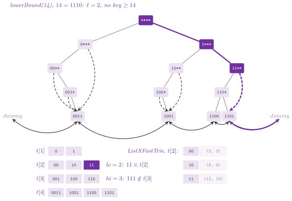
The insertion and the removal are those of the binary trie, which add and remove the entries of the nodes they create and free; they change \(O( w )\) nodes and entries, in \(O( w )\) expected time.
Theorem 7.9. (Morin 2013, Theorem
13.2.) XFastTrie realizes the SSET of
the integers of \(w\) bits, with insert() and remove() in \(O( w )\)
expected time and lowerBound() in \(O( \log w )\) expected time, in
\(O( n w )\) space.
Its tables are FlatHashTables (§7.6), which
compare a fingerprint of the hash with 15 places at once and touch about
one line of cache per lookup, where the book uses its LinearHashTable of
pairs, whose probes compare full keys. The \(\lceil \log_2 ( w + 1 ) \rceil\)
lookups of the binary search depend on each other; hence, the latency of
each one is what counts.
ListXFastTrie is the x-fast trie of Morin 2013, exercise
13.2, with no trie at all. The keys are a
doubly linked list in increasing order, and the table \(t[ i ]\) maps each
prefix of \(i\) bits to the smallest and the largest key with that prefix (an
Entry), which are all that Lemma 7.35 needs.
The binary search finds \(\ell\) as above, and the entry gives the successor
directly. An insertion links the new key before its successor and widens the
entries of its \(w\) prefixes. A removal replaces the smallest key of a prefix
by the next one in the list and the largest by the previous one; this is
correct since the keys of a prefix are consecutive in the list (Algorithm
7.31). find(), lookup() and contains() look
at \(t[ w ]\) alone, in \(O( 1 )\) expected time, seek( x ) gives the iterator
on the successor, as in XFastTrie, and entries() counts the entries of the
tables.
Algorithm 7.31. The successor, the
insertion and the removal of ListXFastTrie (Morin 2013, exercise
13.2); \(t[ i ]( p )\) is the entry of the
prefix \(p\) of depth \(i\), and \(\ell\) the key \(x\) in the list.
Both tries also have findNear( x ), the search of Morin 2013, exercise
13.4, whose time depends on the distance
\(d( x )\) between \(x\) and its successor (\(2^w\) if there is none) rather than on
\(w\) (Algorithm 7.32).
Lemma 7.36. Let
\(k = \lceil \log_2 ( d( x ) + 1 ) \rceil\). Then findNear( x ) takes
\(O( 1 + \log \log d( x ) )\) expected time in ListXFastTrie and
\(O( 1 + \log d( x ) )\) in XFastTrie.
Proof. The successor lies in \([ x , x + 2^k )\), which meets at most two
blocks of \(2^K\) keys aligned to \(2^K\) for each \(K \ge k\), those of the
prefixes \(p = \lfloor x / 2^K \rfloor\) and \(p + 1\) of depth \(w - K\). The
search tries \(K = 1 , 2 , 4 , \ldots\), one or two lookups each, and stops at
the first \(K\) for which one of the two prefixes is there, after
\(O( \log k )\) steps, with \(K < 2 k\). If \(p\) is there, the deepest prefix of
\(x\) lies between the depth \(w - K\) and the depth \(w - K / 2\) of the step
before, where \(p\) was not there, and a binary search finds it in
\(O( \log K )\) lookups. If only \(p + 1\) is there, no key is in the block of
\(x\), and the successor is the smallest key of the block \(p + 1\), which
ListXFastTrie reads from its entry and XFastTrie finds by a walk of
\(K = O( k )\) nodes down the trie. Since \(\log k = O( \log \log d( x ) )\),
the two bounds follow. \(\square\)
In comparison, the hint of the exercise, a scan of the depths from \(w\) upwards, takes \(\Theta( w )\) when the successor is past a carry (\(x = 01 \ldots 1\) and its successor \(10 \ldots 0\), at distance 1, share no prefix), which the block \(p + 1\) covers.
Algorithm 7.32. The search near the
successor of XFastTrie (Morin 2013, exercise
13.4); \(t[ i ]( p )\) is the node of the
prefix \(p\) of depth \(i\), or nil. ListXFastTrie reads the smallest key of
the prefix \(p + 1\) from its entry.
We declare the two x-fast tries as follows.
// declarations of <ADS/dictionary/XFastTrie.h>
template< std::unsigned_integral U , class V = std::monostate ,
          int W = std::numeric_limits< U >::digits >
 requires TrieWidth< U , W >
class XFastTrie : public detail::JumpTrie< U , V , W , true >
{
 using Base = detail::JumpTrie< U , V , W , true >;

 public:
 using Base::Base;
 class const_iterator;
 using Key = U;
 using Item = U;
 using Value = V;
 const U * lowerBound( U x ) const;
 const U * find( U x ) const;
 std::optional< V > lookup( U x ) const;
 bool contains( U x ) const;
 bool insert( U x , const V & v = V() );
 bool remove( U x );
 std::size_t size( void ) const;
 bool empty( void ) const;
 std::size_t nodes( void ) const;
 std::optional< U > min( void ) const;
 std::optional< U > max( void ) const;
 void clear( void );
 const_iterator seek( U x ) const;
 const U * findNear( U x ) const;
 };
template< std::unsigned_integral U , class V = std::monostate ,
          int W = std::numeric_limits< U >::digits >
 requires TrieWidth< U , W >
class ListXFastTrie
{
 public:
 class const_iterator;
 using Key = U;
 using Item = U;
 using Value = V;
 ListXFastTrie( void );
 ListXFastTrie( ListXFastTrie && o );
 ~ListXFastTrie();
 const U * lowerBound( U x ) const;
 const U * find( U x ) const;
 const U * findNear( U x ) const;
 std::optional< V > lookup( U x ) const;
 bool contains( U x ) const;
 bool insert( U x , const V & v = V() );
 bool remove( U x );
 std::size_t size( void ) const;
 bool empty( void ) const;
 std::size_t entries( void ) const;
 const_iterator seek( U x ) const;
 };
7.11.3 The y-fast trie¶
Thus, the x-fast trie is exponentially faster than the binary trie in its
searches, but its updates are not, and its space is \(O( n w )\). These two defects are related, since \(n\) insertions that build a structure of size \(n
w\) take at least that time. YFastTrie (Morin 2013,
§13.3, after Willard
1983) stores in an XFastTrie only a
random sample of the keys, the representatives, each key being one with
probability \(1 / w\) independently of the others, and the key \(2^w - 1\)
always. Hence, the x-fast trie holds \(O( n / w )\) keys in \(O( n )\) space.
The keys between two consecutive representatives, the larger one included,
form a group, kept in a Treap (the alias Group) (Chapter
8) that is the value of its representative in the x-fast
trie. Each key has a group, the one of the smallest representative not
smaller than it (Figure 7.38).
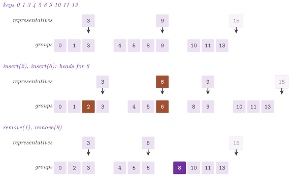
A search of \(x\) finds in the x-fast trie the smallest representative not
smaller than \(x\), in \(O( \log w )\) expected time. It then finds the
smallest key not smaller than \(x\) in its group, by the descent of the treap
(ceiling()), in \(O( \log r )\) expected time for a group of \(r\) keys. An
insertion adds \(x\) to its group and tosses a coin of bias \(1 / w\). If it
comes up, the group is split at \(x\), the keys up to \(x\) go into a new group
whose representative is \(x\), and \(x\) is inserted in the x-fast trie. A
removal takes \(x\) out of its group, and if \(x\) was a representative (other
than \(2^w - 1\)), it joins its group to the next one and removes \(x\) from
the x-fast trie (Algorithm 7.33). The split
and the join of the treaps take \(O( \log w )\) expected time, and the change
of the x-fast trie \(O( w )\), with probability \(1 / w\).
Algorithm 7.33. The successor, the
insertion and the removal of YFastTrie (Morin 2013,
§13.3); \(X\) is the x-fast trie of the
representatives.
In C++, YFastTrie is declared as follows, followed by an example of use.
// declarations of <ADS/dictionary/YFastTrie.h>
template< std::unsigned_integral U , class V = std::monostate ,
          int W = std::numeric_limits< U >::digits >
 requires TrieWidth< U , W >
class YFastTrie
{
 public:
 using Key = U;
 using Item = U;
 using Value = V;
 explicit YFastTrie( std::uint64_t seed = 1 );
 YFastTrie( YFastTrie && o );
 ~YFastTrie();
 const U * lowerBound( U x ) const;
 const U * find( U x ) const;
 std::optional< V > lookup( U x ) const;
 bool contains( U x ) const;
 bool insert( U x , const V & v = V() );
 bool remove( U x );
 std::size_t size( void ) const;
 bool empty( void ) const;
 std::size_t groups( void ) const;
 template< class F >
 void forEach( F && f ) const;
 };
ADS::YFastTrie< std::uint32_t > Y;
for( std::uint32_t x : { 3u , 9u , 12u , 13u } )
 Y.insert( x );
const std::uint32_t * s = Y.lowerBound( 10 );  // *s == 12
The size of the groups rests on two coin experiments (Figure 7.39).
Lemma 7.37. (Morin 2013, Lemma 13.1.) The group of a key \(x\) of a y-fast trie has \(n_x\) keys with \(E[ n_x ] \le 2 w - 1\).
Proof. Let \(x_1 < \cdots < x_i = x < \cdots < x_n\) be the keys. The keys of the group not smaller than \(x\) are \(x_i , \ldots , x_{i+j-1}\), where \(x_{i+j-1}\) is the first of them whose coin came up heads. Hence, \(j\) is at most the number of the tosses of a coin of bias \(1 / w\) up to the first heads, whose expectation is \(w\) (the cut at the last key only lowers it). The keys of the group smaller than \(x\) are \(x_{i-1} , \ldots , x_{i-k}\), all with tails, after the heads of \(x_{i-k-1}\), and hence \(k\) is the number of tails before the first heads of the same experiment, of expectation at most \(w - 1\). Hence \(E[ n_x ] = E[ j ] + E[ k ] \le 2 w - 1\). \(\square\)
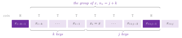
By the inequality of Jensen, \(E[ \log n_x ] \le \log E[ n_x ]\); hence, the operations on a treap of \(n_x\) keys take \(O( \log w )\) expected time. Insertions in the x-fast trie happen with probability \(1 / w\) and cost \(O( w )\), \(O( 1 )\) in expectation, and so do the removals of the representatives.
Theorem 7.10. (Morin 2013, Theorem
13.3.) YFastTrie realizes the SSET of
the integers of \(w\) bits, with insert(), remove() and lowerBound()
in \(O( \log w )\) expected time each (amortized for the first two, the x-fast
trie changing its tables), in \(O( n + w )\) space.
The term \(w\) of the space comes from the representative \(2^w - 1\), which is
always in the x-fast trie (TOP). Our code could avoid it at the price of
some special cases, as Morin remarks, and it keeps it, and therefore each
key has a group. Against the code of the book, the x-fast trie of the
representatives is the one of XFastTrie.h, with its faster tables. The
search in a group descends its treap with no copy of a key, and the coin of
an insertion is one word of SplitMix64 reduced modulo \(w\) instead of a
call to rand(). groups() gives the number of groups, the last one
included, and forEach() visits the pairs by increasing keys. Its invariant (each group between two consecutive representatives, each
representative in its group but the last, and the count of the keys) is
checked in \(O( n )\) time at the contract level 3 while \(n \le 256\).
7.11.4 The binary trie of strings¶
BitmapTrie is the trie of Morin 2013, exercise
13.3, which extends the binary trie from
strings of \(w\) bits to strings of bytes of any length. It is a SORTED SET of
strings, each with a value, whose lowerBound( s ) (the smallest string not
smaller than \(s\) in the lexicographic order of the bytes, a prefix before its
extensions), insert( s ) and remove( s ) take \(O( | s | )\) time, whatever
the number of the strings. The node at depth \(i\) stands for a prefix of \(i\)
bytes, and a string ends at the node of its last byte. The strings are also a
doubly linked list in increasing order, and each node keeps the smallest and
the largest string below it, which play the part of the jump pointers (Figure
7.40). Indeed, the exercise suggests a hash table
of the children in each node. Here a node has instead a bitmap of 256 bits of
the bytes of its children and the children themselves in an array sorted by
byte. Hence, the child of the byte \(c\) is at the rank of \(c\) among the bits
set, a population count as in the hash array mapped tries of Bagwell
2001, with no hashing; the next child
after \(c\) is the next bit set, which a hash table could not give. Methods
has(), rank(), child(), after() and before() are these primitives.
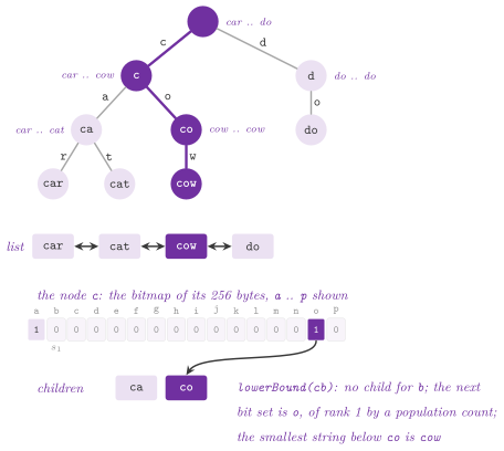
A search that stops at the node \(u\) of depth \(i\), whose child of \(s_i\) is
missing, returns the smallest string below the next child of \(u\), if there
is one. Otherwise it returns the string after the largest one below \(u\), by
the argument of Lemma 7.35 on the bytes, in
\(O( 1 )\) time after the walk of \(O( | s | )\) nodes (Algorithm
7.34). An insertion adds the missing nodes of
the path of \(s\), and links the new string before its successor. Going back
to the root, it makes it the smallest string of each node in which nothing
precedes it (no string ends there and no child has a smaller byte) and the
largest of each node in which nothing follows it. A removal unlinks it,
removes the nodes of its path left empty, and replaces it, where it was the
smallest or the largest string of a node, by the next or the previous one
in the list, since the strings below a node are consecutive in the list.
find(), lookup(), contains(), seek(), size(), empty(),
nodes() and the bidirectional iterators along the list complete the
interface. Its invariant (the list in order, the smallest and the largest
string of each node, the bitmaps) is checked in \(O( N )\) time for \(N\) nodes
at the contract level 3 while there are at most 256 strings.
Algorithm 7.34. The successor, the
insertion and the removal of BitmapTrie (Morin 2013, exercise
13.3); \(u.\mathit{min}\) and
\(u.\mathit{max}\) are the smallest and the largest string below \(u\), and
\(\ell\) the item of \(s\) in the list.
Below are the declarations of BitmapTrie.
// declarations of <ADS/dictionary/BitmapTrie.h>
template< class V = std::monostate >
class BitmapTrie
{
 public:
 class const_iterator;
 using Key = std::string;
 using Item = std::string;
 using Value = V;
 BitmapTrie( void );
 BitmapTrie( BitmapTrie && o );
 ~BitmapTrie();
 const std::string * lowerBound( std::string_view s ) const;
 const std::string * find( std::string_view s ) const;
 std::optional< V > lookup( std::string_view s ) const;
 bool contains( std::string_view s ) const;
 bool insert( std::string_view s , const V & v = V() );
 bool remove( std::string_view s );
 std::size_t size( void ) const;
 bool empty( void ) const;
 std::size_t nodes( void ) const;
 const_iterator seek( std::string_view s ) const;
 };
7.12 Discussion and references¶
Hashing is a large field, and this chapter only touches it; Knuth 1998, §§6.3 and 6.4 remains the reference on the tries and on the classical tables, with the exact analyses of the inspections that §7.5 quotes. The chaining goes back to an internal memorandum of H. P. Luhn at IBM, of January 1953, which seems also to be one of the earliest descriptions of a linked list, and the open addressing to another group at IBM in the same years (Peterson 1957; Morris 1968 surveys the scatter storage of the time). Universal hashing is due to Carter and Wegman 1979, who also introduced the simple tabulation, whose analysis for the linear inspection and the cuckoo hashing is due to Pătrașcu and Thorup 2012. The multiplicative hashing is part of the folklore (Knuth 1998, §6.4), but the random odd multiplier and the analysis of §7.3.3 are due to Dietzfelbinger et al. 1997, and the multiply-add variant, with the collision probability \(1 / 2^d\), to Dietzfelbinger 1996. A faster code for the tuples of fixed length multiplies the parts in pairs, \(\sum_i ( ( x_{2i} + a_{2i} ) \bmod 2^w ) ( ( x_{2i+1} + a_{2i+1} ) \bmod 2^w ) \bmod 2^{2w}\), with half the products of (7.5) and the collision probability \(1 / 2^w\) (Black et al. 1999). The polynomials over a prime field for the sequences are due to Dietzfelbinger et al. 1992, and the reduction modulo a prime \(2^w - 1\) by additions and masks is in Knuth 1998, vol. 2, §3.2.1.1. Attacks by keys chosen to collide, which motivate the random functions, were described by Crosby and Wallach 2003. The engineered tables of §7.6 follow the Swiss tables of Kulukundis 2017 and the table of Boost described by Lopez Munoz 2022; their hash functions borrow from wyhash and XXH3.
The perfect hashing of a static set in linear space is due to Fredman et al. 1984, and its dynamic version to Dietzfelbinger et al. 1994; the cuckoo hashing to Pagh and Rodler 2004, with the stash of Kirsch et al. 2009. Minimal perfect hash functions have been engineered in the last decade toward the bound of Lemma 7.18. Ferragina 2023, chapter 8 is a good entry point to the schemes of §7.8, and Hermann et al. 2024 and Lehmann et al. 2025 report the state of the art at the time of writing.
Skip lists were introduced by Pugh 1990, who also presented their applications and extensions, the finger search and the widths among them (Pugh 1990b). The length of the search path of the \(i\)-th key has been analyzed precisely, with its variance (Papadakis et al. 1992; Kirschenhofer and Prodinger 1994; Kirschenhofer et al. 1995, the last one for the search that saves the comparisons of Lemma 7.28). Also, there are deterministic (Munro et al. 1992), biased (Ergun et al. 2001; Bagchi et al. 2002) and self-adjusting (Bose et al. 2008) versions, and skip lists are used in the indexes of databases, Redis among them, and in the kernel of some operating systems.
Tries are due to Fredkin 1960 and the compact ones to Morrison 1968; the blind search to Ferragina and Grossi 1999, the adaptive radix tree to Leis et al. 2013, and the succinct coding of the trees of higher degree to Benoit et al. 2005. The first structure with the operations of the SSET of the integers in \(O( \log w )\) time is the tree of van Emde Boas 1977, whose space \(2^w\) makes it impractical for large integers. The x-fast and the y-fast tries are due to Willard 1983, the hash tables of the x-fast trie replacing the arrays of the tree of van Emde Boas. Also, the fusion trees of Fredman and Willard 1993 store \(n\) integers of \(w\) bits in \(O( n )\) space with searches in \(O( \log n / \log w )\) time, and the choice between a fusion tree and a y-fast trie, by whether \(\log w > \sqrt{\log n}\), gives searches in \(O( \sqrt{\log n} )\) time in \(O( n )\) space. Lower bounds of Pătrașcu and Thorup 2007 show that these results are more or less optimal for the structures in \(O( n )\) space.
The perfect hash functions of this chapter (MinimalPerfectHash,
RecSplit, FingerprintPerfectHash, PerfectHashTable and
OrderedMinimalPerfectHash) are persistent
(§23.7), as their users typically need, since
they build a function once on a static set of keys and evaluate it for the
life of an index; the file holds the seeds, the pilots, the
codes and the levels, and the template parameters (e.g., the size of the
leaves of RecSplit) are checked on the reading. The dynamic hash tables
are not persistent yet.
7.13 Exercises¶
Each exercise names the test of the library that solves it (run it with
ctest -R <name>). Exercises of Morin
2013 are numbered as in the book; those
that ask to illustrate an operation are solved by the figures of this
chapter, and the others by the lemmas and the code cited.
- Realize a dictionary on the trains numbered from 1 to 36799 and on the
telephone extensions in \([ 280000 , 289999 ]\) with a table with direct
access, every operation in \(O( 1 )\) time, refusing an interval whose
size does not fit in
std::size_t(§7.2). Test:ch07.sec7.direct-access. - Store keys of 8 bits so that every operation costs one access
(Montresor 2025, exercise 7.3).
Test:
ch07.ex7.3. - Realize the DICTIONARY on a sorted vector, with the lookups in
\(O( \log n )\) time and the changes in \(O( n )\) time, and compare it with
std::mapon random operations. Test:beyond.sorted-array-dictionary. - Compute the extraction, the XOR, the division and the multiplication of
§7.3.1 on the examples of Montresor 2025,
§7.1, with the rule of Horner at
the largest \(m\) that does not overflow. Tests:
ch07.sec7.1.functionsandbeyond.hash-examples. - Test the simple uniformity (7.2) by the statistic \(\chi^2\): the division
by a prime against the extraction of the first bits. Test:
ch07.sec7.1.uniformity. - Show that with characters of \(p\) bits and \(m = 2^p - 1\) the division
gives the same place to all the permutations of a key (Montresor 2025,
exercise 7.8). Test:
ch07.ex7.8. - Verify by the enumeration of all the functions of small classes that the
dot products, \(\mathcal{H}_{p,m}\) and the multiply-shift functions
satisfy their bounds of collision (Lemma 7.1 and
§7.3.2). Test:
pearls_hashing.universal-classes. - Measure, on the multiples of \(m\), the mean and the longest list of a
table with lists of overflow and a function of \(\mathcal{H}_{p,m}\)
(§7.4). Test:
pearls_hashing.universal-chaining. - Show that, for any multiplier \(z\) of the multiplicative hashing and
\(n = 2^d\) with \(d \le w / 2\), there are \(n\) keys with the same hash, and
name them given \(z\) (Morin 2013, exercise 5.2);
prove that the bound \(2 / 2^d\) of Lemma 7.3 is reached by \(x = 2^{w-d-2}\)
and \(y = 3 x\) (Morin 2013, exercise 5.3).
Solved in §7.3.3; test:
ods_ints.ods5.1.multiplicative-hash. - Explain why the hash code that reads only the characters of even place,
the XOR and the sum of the two words of a pair, and any deterministic
function of two words into one, have large sets of objects with one
code; explain why
\(( x \bmod 2^w ) + ( x \operatorname{div} 2^w ) \equiv x
\pmod{2^w - 1}\) (Morin 2013, exercises 5.6 to 5.10).
Solved in §7.3.5; test:
ods_ints.ods5.3.hash-codes. - Hash the states of a search by the tables of Zobrist, updating the hash
of a move of the sliding tiles by two XOR, on a state given as a vector,
an array or a span (§7.3.4). Tests:
engineered.random-hashingandengineered_search.zobrist-ranges. - Hash the strings of every length by the folded products, with the same
hashes with and without the kernels of Highway, and check that
a flip of one bit of a key flips about half of the bits of its hash
(§7.3.6). Test:
hashing.fast-hash. - Fingerprint the rows of doubles, \(+0\) equal to \(-0\) and all the NaNs
equal, and confirm the matches by
sameRow(). Test:engineered_sparse.row-fingerprint. - Bring to the head of their list the keys looked up often (Montresor
2025, exercise 7.5). Test:
ch07.ex7.5. - Keep the lists of overflow sorted, and measure the accesses of the
unsuccessful searches against those of the lists that are not
(Montresor 2025, exercise 7.10).
Test:
ch07.ex7.10. - Search a list of long keys with their hashes, comparing a key only when
its hash is equal (Montresor 2025, exercise
7.7). Test:
ch07.ex7.7. - Find the replicated files of a file system in \(O( n )\) expected time by
a table from the content to the paths (Montresor 2025, exercise
7.6), and remove the duplicates
of an unsorted vector in \(O( n )\) expected time (Montresor 2025,
exercise 7.9). Tests:
ch07.ex7.6andch07.ex7.9. - Compute the codomain of a dictionary on a tree and on the two hash
tables (Montresor 2025, exercise 8.8).
Test:
ch08.ex8.8. - Compare the hash tables of §7.4 and
§7.5 with
std::map, with and without restructuring, and measure \(I( \alpha )\) and \(S( \alpha )\) against (7.7) and Table 7.2. Tests:ch07.sec7.2.against-mapandch07.sec7.3.complexity. - Show that a sequence that alternates an insertion and a removal at the
threshold restructures the table only once with the thresholds 4 times
apart (Lemma 7.7). Test:
ch07.sec7.4.restructure. - Realize the table of Morin 2013, §5.1
with the multiplicative hashing on \(2^d\) lists, which doubles past the
load 1 and halves below \(1 / 3\) (Theorem 7.3), and show that the keys
\(k \cdot 2^{20}\) spread over it while \(h( k ) \bmod m\) would put them in
one list. Explain whether the first two or the last two digits of the
student numbers of a class of first year students make a better hash
(Morin 2013, exercise 5.1), and how
the keys of a table with a fixed hash can be chosen to make its searches
linear (Morin 2013, exercise 5.11).
Solved in §7.5; test:
ods_ints.ods5.1.chained-hash-table. - Insert, remove and insert again the keys of the exercise in a table of
11 places with the linear inspection, up to the full table (Montresor
2025, exercise 7.1). Test:
ch07.ex7.1. - Show that the inspection \(( k \bmod 11 + 3 i + i^2 ) \bmod 11\) is not a
permutation and that an insertion fails while a place is free
(Montresor 2025, exercise 7.2),
and write the procedures of the linear and of the quadratic inspection
(Montresor 2025, exercise 7.4).
Tests:
ch07.ex7.2andch07.ex7.4. - Show that a deleted place does not stop an inspection and that an
insertion reuses it (Montresor 2025, Figure
7.6). Test:
ch07.sec7.2.deleted. - Show that the triangular inspection visits every place of a table of
\(2^p\) places (Lemma 7.9), and realize the double hashing with a second
function. Test:
beyond.hashing. - Realize the
LinearHashTableof Morin 2013, §5.2 with the tabulation hashing (Theorem 7.4); reprove Lemma 7.10 with the full formula of Stirling (Morin 2013, exercise 5.4); and explain why storing a key in the first nil place, skipping the deleted ones, makes \(O( n )\) operations take \(\Theta( n^2 )\) time (Morin 2013, exercise 5.5). Solved in §7.5; test:ods_ints.ods5.2.linear-hash-table. - Realize the coalesced hashing with a cellar and the double hashing with
the insertion of Brent, whose successful searches take fewer than 2.5
probes on average in a table 95 % full. Test:
taocp.knuth-hashing. - Measure the longest list of the d-left hashing for \(d = 1 , 2 , 4\) with
\(n = m\) keys. Test:
pearls_hashing.d-left. - Realize the table with control bytes in groups of 15 against
std::unordered_map, on keys that all share one fingerprint, on groups that wrap around the end and with the broadword fallback (§7.6). Test:engineered.flat-hash-table. - Realize the hash map with its pairs in a dense vector and an index of
positions. Test:
hashing.dense-hash-map. - Realize the closed list of a search as a table of pointers with their
hashes, presized by
slotsFor(), on hashes biased in their low bits. Tests:engineered.pointer-tableandengineered_search.pointer-table-presize. - Renumber the positions of an index after the erasure of some of them, in
one pass over the table. Tests:
engineered_sparse.position-indexandengineered_sparse.position-index-renumber. - Realize the cuckoo hashing with a stash, and check that a table of
\(m \ge 6 n ( 1 + \epsilon )\) places needs no rehash in at least half of
the builds (Lemma 7.15). Tests:
pearls_hashing.cuckooandpearls_hashing.cuckoo-analysis. - Realize the cuckoo hashing with buckets of 4 places and a search in
breadth, and reach a load above 0.9 with no growth. Test:
hashing.bucket-cuckoo. - Build the two-level perfect hashing of the example of Ferragina 2023,
Figure 8.6 and of random sets,
with fewer than \(4 n\) places in the second level (Lemma 7.17). Tests:
pearls_hashing.fks-exampleandpearls_hashing.fks-table. - Label the graph of Ferragina 2023, Table 8.1
and build the order preserving minimal perfect hash with \(r = 2\) and
\(r = 3\) (Lemma 7.19). Tests:
pearls_hashing.opmphf-exampleandpearls_hashing.opmphf. - Build the minimal perfect hash functions by pilots, by fingerprints and
by recursive splitting, and check that they are bijections onto
\(\{ 0 , \ldots , n - 1 \}\) (§7.8.3).
Tests:
hashing.minimal-perfect-hash,hashing.fingerprint-perfect-hashandhashing.recsplit. - Illustrate the searches of 2.5 and of 5.5, the insertions of 0.5 with a
height of 1 and of 3.5 with a height of 2, and the removals of 1 and of
3 on the skip list of Morin 2013, Figure 4.1
(Morin 2013, exercises 4.1 to 4.3);
show that an insertion or a removal changes a constant number of links
in expectation (Morin 2013, exercise 4.6).
Solved by Figure 7.21,
Figure 7.22,
Figure 7.23 and Lemma 7.24; test:
ods_trees.ods4.2.skiplist-sset. - Illustrate
remove( 2 )andadd( 3 , x )with a height of 4 on the skip list with the lengths of Morin 2013, Figure 4.5 (Morin 2013, exercises 4.4 and 4.5), and realize the skip list with the access by rank (Morin 2013, exercise 4.9). Solved by Figure 7.25 and Lemma 7.30; tests:ods_trees.ods-ex4.9.rank-skiplistandods_trees.ods4.3.skiplist-list. - Promote the keys with a probability \(p\) instead of \(1 / 2\): bound the
search path, the height and the nodes, and find the best \(p\) (Morin
2013, exercise 4.7). Solved by
Lemma 7.27; test:
ods_trees.ods4.2.skiplist-sset. - Remove the redundant comparisons of the search of a skip list, and
count the comparisons of the new search (Morin 2013, exercise
4.8). Solved by Lemma 7.28; test:
ods_trees.ods-ex4.8.no-redundant-comparisons. - Realize the finger search of a skip list, in \(O( 1 + \log r )\) expected
time (Morin 2013, exercise 4.10).
Solved by Lemma 7.29; test:
ods_trees.ods-ex4.10.finger-search. - Truncate a
SkiplistListat a position and absorb another one, in \(O( \log n )\) time (Morin 2013, exercises 4.11 and 4.12), in Chapter 2. Test:ods_trees.ods-ex4.11.truncate-absorb. - Design the space-efficient SSET on a space-efficient list of blocks
(Morin 2013, exercise 4.13), in
Chapter 10. Test:
ods_trees.ods-ex4.13.sesset. - Search the substrings of a text interactively by an SSET of its
suffixes (Morin 2013, exercise 4.14).
Test:
ods_trees.ods-ex4.14.substring-search. - Explain how removing some links of a skip list leaves a binary tree
similar to a binary search tree, and why the skip list uses its links
better (Morin 2013, exercise 4.15).
Solved in §7.9.6 and by
Figure 7.26; tests:
taocp.balanced-treesandods_trees.ods4.2.skiplist-sset. - Realize the trie and the compact trie of strings, with keys that are
prefixes of one another and removals inside a chain of prefixes. Test:
taocp.tries. - Run the blind search on the Patricia trie of Ferragina 2023, Figures
9.7 and 9.8, and put it over the
front coding of a dictionary (Lemma 7.32). Tests:
pearls_hashing.patriciaandpearls_hashing.two-level. - Realize the adaptive radix tree on strings, with values that own
memory. Test:
ordered.adaptive-radix-tree. - Code a static dictionary of strings as a Patricia trie in DFUDS, with
access()andlookup()inverse of each other (Lemma 7.34). Test:engineered_strings.string-dictionaries. - Realize the binary trie of the integers of \(w\) bits (Theorem 7.8).
Test:
ods_ints.ods13.1.binary-trie. - Design a binary trie with neither the list nor the jump pointers whose
find( x )still runs in \(O( w )\) time (Morin 2013, exercise 13.1). Test:ods_ints.ods.ex13.1.simple-binary-trie. - Realize the x-fast trie (Theorem 7.9), and design one with no binary
trie, only a doubly linked list and \(w + 1\) hash tables (Morin 2013,
exercise 13.2). Tests:
ods_ints.ods13.2.x-fast-trieandods_ints.ods.ex13.2.list-x-fast-trie. - Extend the binary trie to the strings of any length, with the
operations in time proportional to the length of the string (Morin
2013, exercise 13.3). Test:
ods_ints.ods.ex13.3.bitmap-trie. - Modify the search of an x-fast trie so that it runs in
\(O( 1 + \log d( x ) )\) and in \(O( 1 + \log \log d( x ) )\) expected time,
\(d( x )\) the distance of \(x\) from its successor (Morin 2013, exercise
13.4). Solved by Lemma 7.36; test:
ods_ints.ods.ex13.4.find-near. - Realize the y-fast trie (Theorem 7.10 and Lemma 7.37). Test:
ods_ints.ods13.3.y-fast-trie.