22. Succinct structures¶
[Source: include/ADS/succinct/BitVector.h, BitStream.h,
RankSelect.h, CompactRankSelect.h, InterleavedRankSelect.h,
RRRBitVector.h, EliasFano.h, PartitionedEliasFano.h, LAVector.h,
PackedArray.h, JacobsonTree.h, LoudsTree.h, BalancedParentheses.h,
BPTree.h, WaveletMatrix.h, HuffmanWaveletTree.h, MoveStructure.h,
EliasFanoGraph.h, BVGraph.h, K2Tree.h]
We are concerned in this chapter with the data structures that take about
as many bits as the information they hold, and that answer their queries
without being decoded. The headers of ADS/succinct follow chapter 15,
Compressed Data Structures, of Ferragina 2023,
and the representation of Elias and Fano of its chapter 11, Integer
Coding; the book of Montresor does not treat them. Both operations on which all of them are built, the rank and the select of a vector of bits,
are defined in §22.1 together with the lower
bounds against which the space is measured. We then give the vector of
bits and the streams of bits (§22.2), the
directories of rank and select, from the fastest to the smallest
(§22.3 and §22.4),
and the vector compressed to its entropy
(§22.5). On them we build, in turn, the sequences of integers searched in place (§22.6), the arrays
of small fields (§22.7), the trees
(§22.8), the sequences of symbols and the
permutations (§22.9) and the graphs (§22.10). Finally, §22.11 describes how the directories and the wavelet structures are built on
several threads. In the sets of §1.9,
CompactRankSelect.h, InterleavedRankSelect.h, LAVector.h,
MoveStructure.h, PackedArray.h, PartitionedEliasFano.h,
RRRBitVector.h and WaveletMatrix.h are advanced and the other headers
of this chapter are base.
Some members are common to the classes of the chapter, and we describe
them once here. All the static sequences (BitVector, the directories of
RankSelect.h and CompactRankSelect.h, EliasFano,
PartitionedEliasFano, LAVector and WaveletMatrix) are random-access
ranges with the aliases of the standard containers (value_type,
size_type, difference_type, reference, const_reference,
const_iterator and iterator, the same), whose iterators read the items
by subscript (SubscriptIterator of BitVector.h), from begin() and
cbegin() to end() and cend(). Each structure gives its space in bits
by sizeInBits(); besides, the directories give their bits beyond those
of the vector by directoryBits(), EliasFano and BVGraph the bits of
their codes alone by codeBits(), BalancedParentheses the bits of its
range min-max tree by treeBits(), and LAVector the bits of its
corrections by correctionsInBits() (and their width by
correctionBits()). Finally, the trees mark a missing node (or place) by
the constant nil.
22.1 Rank, select and the lower bounds¶
A vector of bits \(B[ 0 , m )\) with \(n\) 1s has, for \(b \in \{ 0 , 1 \}\), the operations
i.e., the number of the bits \(b\) before the place \(i\) (cf. (22.1)), and the place of the \(k\)-th bit \(b\), with \(1 \le k\) up to the number of the bits \(b\). Hence \(\mathrm{rank}_b( \mathrm{select}_b( k ) ) = k - 1\), and \(\mathrm{rank}_0( i ) = i - \mathrm{rank}_1( i )\). We count the places from 0, as the library does, while Ferragina's book counts them from 1; its \(\mathrm{Rank}_1\) and \(\mathrm{Select}_1\) are therefore our \(\mathrm{rank}_1\) and \(\mathrm{select}_1\) with the places shifted by one. We regard the two operations as the primitives of the area: a structure that codes its objects as bits uses the select to go from the number of an object to its place in the bits, and the rank to go back.
A representation of the objects of a class of \(N\) elements needs \(Z = \lceil \log_2 N \rceil\) bits for some of them, the information-theoretic lower bound. We call it succinct if it takes \(Z + o( Z )\) bits, and compact if it takes \(O( Z )\) bits. In both cases it should answer its queries in about the time of the plain representation (possibly up to a constant). Three bounds recur in the chapter. The vectors of \(m\) bits with \(n\) 1s are \(\binom{m}{n}\). Similarly, the sets of \(n\) integers of \([ 0 , u )\) are \(\binom{u}{n}\), i.e., about \(n \log_2( u / n ) + n \log_2 e\) bits when \(n\) is much smaller than \(u\). Finally, the ordered trees of \(n\) nodes (and the binary trees of \(n\) nodes) are the Catalan number \(C_n = \binom{2 n}{n} / ( n + 1 ) \approx 4^n / ( n^{3/2} \sqrt{\pi} )\), i.e., \(2 n - \Theta( \log n )\) bits.
Lemma 22.1. With \(H_0( B ) = \frac{n}{m} \log_2 \frac{m}{n} + \frac{m - n}{m} \log_2 \frac{m}{m - n}\), the empirical entropy of a vector of \(m\) bits with \(n\) 1s,
Proof. With \(p = n / m\), one has \(\binom{m}{n} p^n ( 1 - p )^{m - n} \le \sum_k \binom{m}{k} p^k ( 1 - p )^{m - k} = 1\), and the logarithm of \(p^{-n} ( 1 - p )^{-( m - n )}\) is \(m H_0( B )\). \(\square\)
Table 22.1 collects the notation of the area. We analyze the costs in the model of the word RAM with words of \(\Theta( \log m )\) bits, in which the sideways sum of a word (the number of its 1s, \(\lvert x \rvert\) or \(\mathrm{popcount}( x )\)) and the place of its \(k\)-th 1 cost \(O( 1 )\) time. Indeed, the first is one instruction of today's processors, and the second a few broadword operations (§22.2).
Table 22.1. The notation of the chapter.
| Symbol | Meaning |
|---|---|
| \(B\), \(m\), \(n\) | a vector of bits, its length and the number of its 1s |
| \(\mathrm{rank}_b( i )\), \(\mathrm{select}_b( k )\) | as in (22.1); rank1(), select1(), rank0(), select0() in the code |
| \(H_0\) | the empirical entropy of order 0 of a vector of bits, or of a sequence of symbols of frequencies \(f_c\), \(\sum_c ( f_c / n ) \log_2( n / f_c )\) |
| \(x_0 , \ldots , x_{n-1}\), \(u\) | a non-decreasing sequence of integers, and the bound of its items |
| \(\ell\), \(L\), \(H\) | the low bits of an item of Elias-Fano, and the vectors of the low and of the high parts |
| \(\sigma\), \(w\) | the size of an alphabet of symbols, and the bits of a symbol of a wavelet matrix |
| \(E( i )\) | the excess of a sequence of parentheses, the open ones less the closed ones in \(B[ 0 , i ]\) |
| \(\lvert x \rvert\), \(\mathrm{popcount}( x )\) | the number of the 1s of a word |
22.2 Vectors of bits and streams¶
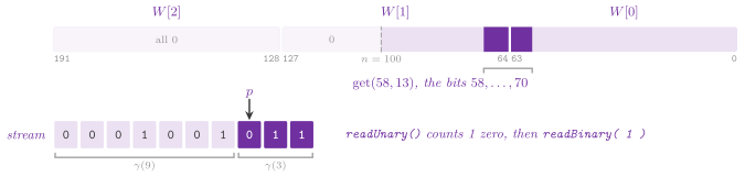
BitVector packs the bits in words of 64 bits, the bit \(i\) in the bit
\(i \bmod 64\) (from the least significant one) of the word
\(\lfloor i / 64 \rfloor\) (Figure 22.1). Besides the access to a bit in \(O( 1 )\) time, the class appends a bit or a field of up to
64 bits (push_back() and append()) in \(O( 1 )\) amortized time, and it
reads a field of up to 64 bits (get()) in \(O( 1 )\) time with two shifts
at most (Algorithm 22.1). Its words fill lines of the cache of 64 bytes, with at least one word past the last bit. They start on a line (on a huge page from 2 MB on, which may spare the misses of the TLB of a random access), and the space is therefore \(m + O( 512 )\) bits for \(m\) bits. We keep the bits past the size at 0, which is the invariant of the class. For this reason a field is read with no test of the end, and the
rank of a word needs no mask at the end of the vector. Unlike
std::vector< bool >, whose layout is left to the implementation,
BitVector exposes its words, which a directory of rank or a code read a
word at a time needs. Its words are a Words, a vector on the allocator of
the lines; copyBits() ors a run of bits of a word array into another
from any place, reserve( n ) makes room for \(n\) bits and toString()
writes the bits as '0' and '1', the bit 0 first.
Algorithm 22.1. The append and the read of
a field of BitVector; \(W\) are the words.
Finding the place of the \(k\)-th 1 of a word, by selectInWord(), is the last step of
each select of the library, in place of the tables of the small blocks of
the classical analysis (Jacobson 1989;
Clark 1996). It is the broadword method
of Vigna 2008
(Algorithm 22.2), with
\(L_8 = \sum_{j < 8} 2^{8 j}\) and \(H_8 = 2^7 L_8\).
Algorithm 22.2. The broadword select in a word (Vigna 2008).
Lemma 22.2. Let \(s_j\) be the number of the 1s of the bytes \(0 , \ldots , j\) of \(x\), and \(k < \lvert x \rvert\). The byte \(j\) of \(s + ( 127 - k ) L_8\) has its high bit if and only if \(s_j > k\), and the first such byte holds the \(k\)-th 1 of \(x\), counting from 0.
Proof. Since the sideways sums of the 8 bytes are at most 8, one product by \(L_8\) puts their prefix sums \(s_j \le 64\) in the bytes, and no byte overflows, since \(s_j < 256\). Adding \(127 - k\) to the byte \(j\) gives at most \(64 + 127 < 256\), and therefore no carry crosses into the next byte; the sum is at least 128, i.e., it has its high bit, if and only if \(s_j \ge k + 1\). Hence the first byte \(b\) with \(s_b > k\) is the one that holds the 1 of rank \(k\), which is the \(( k - s_{b-1} )\)-th 1 of the byte. \(\square\)
In the implementation, the trailing zeros of the masked word give \(b\), and
the 1 inside the byte is read in a table of \(256 \cdot 8\) bytes, indexed by
the byte and by the rank in it, as in Vigna
2008. The select has thus neither a loop
nor an instruction of a particular processor, while the deposit of the bit
\(2^k\) on the 1s of the word (the instruction pdep of BMI2) would need a
branch on the processor.
We write the codes of the integers of §21.7
on the streams of bits of BitStream.h. A BitWriter appends
bits to a BitVector, and a BitReader reads them back from a place that
moves forward, both in \(O( 1 )\) time per field of up to 64 bits
(Algorithm 22.3). The functions write() and read() move a field with its least significant bit first, the order of the words. The functions writeBinary() and readBinary() move it with its most significant bit first, the order in which the codes are written on paper, and they turn the field around by three rounds of masks and a swap of the bytes. Also,
writeUnary( q ) writes \(q\) zeros and a 1, and readUnary() counts the
zeros up to the 1 a word at a time, by the trailing zeros of the word, in
\(O( 1 + q / 64 )\) time. A single bit is moved by writeBit() and
readBit(); seek( p ) moves the reader to the place \(p\), atEnd()
is true when all the bits have been read, and release() hands the bits
written over to the caller, leaving the writer empty. In the literature the fast decoders write the codes into words rather than bytes, e.g., the streams of the WebGraph framework of Boldi and Vigna 2004. Indeed, a codeword of up to 64 bits spans at most two words, and the unary part is
decoded by one instruction per word.
Algorithm 22.3. The binary and the unary fields of the streams of bits.
Lemma 22.3. (i) A BitVector of \(m\)
bits keeps at most \(\lfloor m / 64 \rfloor + 10\) words, i.e., \(m + O( 512
)\) bits, with at least one word past the last bit and the bits past the
size at 0. (ii) get( i , len ), \(len \le 64\), reads at most two words,
and push_back() and append() take \(O( 1 )\) amortized time. (iii)
readUnary() reads \(q\) zeros and the 1 in at most \(\lfloor q / 64 \rfloor
+ 1\) steps of one word each.
Proof. (i) The constructor of \(m\) bits takes \(\lceil ( \lfloor m / 64
\rfloor + 9 ) / 8 \rceil 8 \le \lfloor m / 64 \rfloor + 9\) words, rounded
down to a multiple of 8, i.e., at least \(\lfloor m / 64 \rfloor + 2\); an
append grows the words by 8 only when fewer than \(\lfloor m' / 64 \rfloor
+ 2\) are there for the new size \(m'\), which keeps the count below
\(\lfloor m' / 64 \rfloor + 10\). The constructor writes 0s past the size,
and an append writes only the bits of its field, whose value has no 1
above its length (a precondition). (ii) A field of at most 64 bits from
the place \(i\) lies in the words \(\lfloor i / 64 \rfloor\) and the next
one. An append writes at most two words, and the growth of the words by 8
at a time reallocates them geometrically (the growth of std::vector
beyond its capacity), which is \(O( 1 )\) amortized per append. (iii) Each
step reads up to 64 bits from the current place: if they are all 0 it
counts them and moves past them, and otherwise the trailing zeros of the
word give the 1. All the steps but the last read 64 zeros each (or the
last bits of the vector, after which the precondition stops the reader).
\(\square\)
22.3 Rank and select¶
One can reduce the rank to a few counts by the two-level directory of Jacobson.
Lemma 22.4 (the directory of Jacobson). With superblocks of \(Z\) bits, each with the 1s before it in \(\log_2 m\) bits, and blocks of \(z\) bits, each with the 1s before it since its superblock in \(\log_2 Z\) bits,
and with \(Z = \log_2^2 m\) and \(z = \log_2 m / 2\) the counts take \(o( m )\) bits, with the rank in \(O( 1 )\) time.
Proof. The places before \(i\) are split into those before its superblock, those of its superblock before its block, and those of its block before \(i\); counting the 1s of each part gives the three terms of (22.3). Also, the superblocks take \(( m / \log_2^2 m ) \log_2 m = m / \log_2 m\) bits, and the blocks \(( 2 m / \log_2 m ) \log_2 \log_2^2 m = O( m \log \log m / \log m )\), both \(o( m )\). Finally, the last term of (22.3) is read in a table of the \(2^z = \sqrt{m}\) blocks of \(z\) bits and of their \(z\) prefixes, of \(O( \sqrt{m} \log m \log \log m )\) bits. \(\square\)
In the library we replace the table by the sideways sum of a word, one
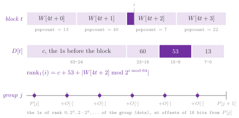
instruction of the processor, which lets \(z\) be a word and \(Z\) a constant. RankSelect (chapter 15 of
Ferragina 2023) keeps one word for
each block of 256 bits: the 1s before the block in its 40 high bits, and
those before its words 1, 2 and 3, relative to the block, in 8 bits each
(Figure 22.2). Hence one can compute (22.3) by one read of the directory and one of the bits, with no branch, at the price of
\(64 / 256 = 25\%\) of space more instead of \(o( m )\)
(Algorithm 22.4). This fraction is constant, but it is "small" at the practical sizes, since \(m / \log_2 m\) is still 2.5% of \(m\) for \(m = 2^{40}\), a "large" vector. Above \(2^{40}\) bits, a third level counts the 1s
before each \(2^{40}\) bits in 64 bits.
Algorithm 22.4. The directory of
RankSelect and its rank, with the blocks of 256 bits.
We build the directory in one pass on the words. Here the sideways sums \(p_0 , \ldots , p_3\) of the words of a block, at most 64 each, are put in the bytes of a word, and one product gives their prefix sums in the bytes, which do not overflow,
i.e., the three relative ranks of the entry. When the bits come from words in memory above \(2^{23}\) bits, the words are copied in the same pass, since reading them twice costs more than a copy in the caches. The implementation follows the pseudocode. Note that the 1s of the word up to \(i\) need no test of the end, since the words exist past the size.
We do not reduce the select to the rank by a binary search, which would cost \(O( \log m )\) steps. Clark 1996 cuts the
1s in groups of \(\log_2^2 m\) and writes down the places of all the 1s of a
group that spans more than \(\log_2^4 m\) bits; these take
\(O( m / \log m )\) bits in all, since such groups are at most
\(m / \log_2^4 m\). All the other groups are cut again, and the last level is solved by a table. This gives \(O( 1 )\) time in \(o( m )\) bits, at the price of three levels whose constants are rather large at the sizes of the practice.
We follow instead the inventories of the simple select of
Vigna 2008, with groups of constant
size, for the 1s and for the 0s. We cut the 1s in groups of \(2^\ell\), with
\(\ell = \lfloor \log_2( 1.5 \cdot 4096 \, k / m ) \rfloor\) for \(k\) of them,
and a group thus spans between 3072 and 6144 bits on average. For each group
the place of its first 1 is kept in 64 bits, and the places of its 1s of
rank multiple of \(2^g\), \(g = \max\{ \ell - 5 , 0 \}\), in 16 bits from it,
i.e., at most 32 offsets, a line of the cache. Hence \(\mathrm{select}_1( k )\) reads the place of the 1 of rank \(k - 1\) rounded down to a multiple of \(2^g\). It counts the rest of the 1s word by word, by the sideways sums, and it ends in the word by selectInWord() (Algorithm 22.5).
Algorithm 22.5. The select of RankSelect
by the inventories of Vigna 2008.
Lemma 22.5. (i) The entries of
Algorithm 22.4 hold the 1s before each block and
the relative ranks of its words 1 to 3 without overflow, (22.4) gives the
latter, and rank1( i ) is their sum plus the 1s of the word of \(i\) before
\(i\). (ii) For \(1 \le k \le n\), Algorithm 22.5
returns \(\mathrm{select}_1( k )\); in a group that is not sparse it reads
fewer than \(2^{16} / 64 + 1\) words of the vector, and in a sparse one it
makes \(O( \log( m / 256 ) )\) steps. (iii) The directory of rank takes 64
bits per 256 bits of the vector, and the inventory of the 1s 64 bits per
group and at most 32 offsets of 16 bits.
Proof. (i) The relative ranks are at most \(3 \cdot 64 = 192\), which fit
in 8 bits; in (22.4) each partial sum is at most 192, so that no byte
carries into the next one, and the product modulo \(2^{24}\) leaves in the
byte \(j\) the sum \(p_0 + \cdots + p_j\). The rank of \(i\) in the word \(q\) of
its block is then the 1s before the block, plus the relative rank of \(q\)
(0 for \(q = 0\)), plus the 1s of the word \(q\) before \(i\), which is (22.3)
with the word as the last block. (ii) The 1 of rank \(r = k - 1\) (from 0)
is in the group \(j = \lfloor r / 2^\ell \rfloor\). If the group is sparse,
its 1 is found by a binary search on the counts of the directory between
the places of the first 1s of the groups \(j\) and \(j + 1\), over at most \(m
/ 256\) blocks. Otherwise line 5 gives the place \(p\) of the 1 of rank \(2^g
\lfloor r / 2^g \rfloor \le r\), which is \(r\) itself for \(g = 0\). The 1 of rank \(r\) is the \(t\)-th 1, from 0, at or after \(p\), with \(t = r \bmod 2^g\),
and the loop of line 8 skips the words that hold fewer than \(t + 1\) of the
1s still to pass, until selectInWord() finds it
(Lemma 22.2). The 1s from \(p\) to the 1 of rank
\(r\) lie in the group, which spans fewer than \(2^{16}\) bits since it is not
sparse; hence the loop reads fewer than \(2^{16} / 64 + 1\) words. (iii) A
group of \(2^\ell\) 1s keeps its first place in 64 bits and the offsets of
its 1s of rank multiple of \(2^g\), at most \(2^{\ell - g} \le 32\) of them, in
16 bits each. \(\square\)
On bits spread evenly, a group spans between 3072 and 6144 bits on average by the choice of \(\ell\), and the scan of line 8 then covers a few words; this, and not (ii), is the case for which the inventories are designed.
A select is thus (typically) three accesses to the memory and a few words, \(O( 1 )\) time where the 1s are spread evenly, with about \(576 / 6144\) to \(576 / 3072\), i.e., 9.4% to 18.8%, of \(m\) bits more for each value. A group that spans \(2^{16}\) bits or more (quite a "sparse" one) has offsets that do not fit in 16 bits; it is sparse, and its 1s are found by a binary search on the directory of rank between its ends, \(O( \log( m / 256 ) )\) time in the worst case. A group that spans less is scanned over fewer than \(2^{16} / 64 = 1024\) words, and usually over a few, as long as the bits are not "clustered". Also, a group of fewer than 32 bits \(b\) (below about 1% of them) keeps the place of each one, and its select reads no bit at all. These are the trade-offs of the practical designs: we find them in the rank9 and the inventories of Vigna 2008, in the darray of Okanohara and Sadakane 2007, and in the structures of Gog and Petri 2014.
We build the inventories of select in the constructor (RankSelect, the default), or at the first select of each value (LazyRankSelect), in a pass on the directory. A structure that only ranks then never pays for them; also, a RankSelectOptions::Selects asks for the selects of the 1s,
of the 0s, of both or of neither. Note that the first call builds an inventory once,
whichever thread calls it, with std::call_once and a flag read with
acquire semantics before it, and a copy keeps the inventories already
built. We remark that the lazy form may cost the select 10 to 15%, since the load of the flag with acquire semantics makes the compiler read the fields of the inventory again at each query, whereas the eager form (the template parameter Lazy false) keeps them in plain fields.
22.4 Compact and interleaved directories¶
RankSelect spends about 50% of \(m\) bits (with both selects) for the
fastest queries. CompactRankSelect is its compact counterpart, the flat
directory of Kurpicz 2022, after the
poppy of Zhou, Andersen and Kaminsky 2013,
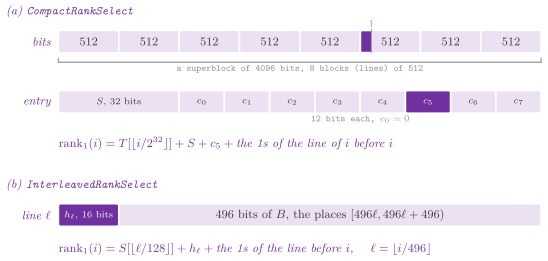
in about 3.5% of \(m\) bits. It cuts the bits in superblocks of 4096 bits,
each one in 8 blocks of 512 bits, a line of the cache. One entry of 128
bits per superblock holds the 1s before it since its top region of
\(2^{32}\) bits, in 32 bits, and the 1s before each of its blocks since the
superblock, \(c_0 = 0 , c_1 , \ldots , c_7 \le 3584\), in 12 bits each; a
count of 64 bits per top region completes the rank
(Figure 22.3). Hence
with \(o = i \bmod 512\) and \(w_j\) the words of the block: one access to the
entries, one to the line of the block, and the sideways sums of its 8 words
cut at \(i\), with no branch (Algorithm 22.6).
With Highway, we cut the 8 words of the line at \(i\) and count them a vector at a time, the masks of the words made from the lanes of \(\mathrm{clamp}( i - 64 j , 0 , 64 )\), by the count of the lanes of Highway (Mula, Kurz and Lemire 2018). We compute the sum on the line by one kernel of BitVector.h, detail::lineRank(), whose variants (the one on Highway, and the scalar one with or without BMI2) are chosen by ADS_WITH_HIGHWAY and by the target, and which InterleavedRankSelect below calls on the lines that hold its counts. In all, the entries take \(128 / 4096 = 3.125\%\) of \(m\) bits.
Algorithm 22.6. The rank and the select of
CompactRankSelect (Kurpicz 2022).
Its select keeps the superblock of each 4096-th bit \(b\), in 32 bits each,
i.e., at most \(32 / 4096 < 0.8\%\) of \(m\) bits for each value. It finds the \(k\)-th bit \(b\) by a binary search on the entries between two samples. Then it finds the block by the 7 counts of the superblock, and the word by the sums of the 8 words of its line, both by comparisons with no branch; the bit is found by selectInWord(). This is \(O( \log( m / 4096 ) )\) steps in the worst case,
and \(O( 1 )\) where the bits \(b\) are spread "evenly" (a sample each 2 to 8 superblocks for a density between 1/2 and 1/8). Its trade with RankSelect is, roughly, the "classical" one of the literature: a sum of up to 8 words and a
search of the entries instead of one word and an inventory, in 15 times
fewer bits.
InterleavedRankSelect takes the layout of SPIDER of
Laws et al. 2024, with the counts inside
the lines of the bits. A line of 512 bits holds 496 bits of \(B\). In its first 16 bits it holds the 1s before it since its superblock of 128 lines (63488
bits, so that the count fits in 16 bits); a superblock keeps the 1s before
it in 64 bits apart. Hence
with one access to the memory of the vector, the line, against the two of the directories kept apart. Its array of the superblocks, one word per 63488 bits, typically stays in the caches, and the counts take \(16 / 512 = 3.125\%\) of the line. Its select keeps the line of each 8192-th bit \(b\) with the bits \(b\) before that line, in 96 bits, i.e., at most \(96 / 8192 < 1.2\%\) of \(m\) bits for each value. As SPIDER does, it guesses the line of the \(k\)-th bit \(b\) between two samples \(( \ell_j , c_j )\) by interpolation,
and then corrects the guess a line at a time by the counts of the lines (hopefully a step or two where the bits \(b\) are spread evenly, but \(\ell_{j+1} - \ell_j\) in the worst case). It ends in the line by the sums of its words and
selectInWord() (Algorithm 22.7).
Algorithm 22.7. The rank and the select of
InterleavedRankSelect
(Laws et al. 2024).
Lemma 22.6. (22.5) and (22.6) give
\(\mathrm{rank}_1( i )\), and their counts fit in the fields that hold them;
the entries of CompactRankSelect take \(128 / 4096\) of the bits and the
counts of InterleavedRankSelect \(16 / 512\) of each line.
Proof. In (22.5), the places before \(i\) are split into four parts. They are those before its top region of \(2^{32}\) bits, those of the region before its superblock, those of the superblock before its block, and those of the block before \(i\); the last term counts the 1s of the words \(j\) of the block whose bits \(64 j , \ldots\) precede \(o\), all of them when \(o \ge 64 ( j + 1 )\) and none when \(o \le 64 j\). The count of a superblock is below \(2^{32}\), and \(c_j \le 7 \cdot 512 = 3584 < 2^{12}\). In (22.6) the places before \(i\) are those before its superblock of 128 lines, those of the lines of the superblock before the line \(\ell\), and those of the line before \(i\); the count \(h_\ell\) is at most \(127 \cdot 496 = 62992 < 2^{16}\). A superblock of 4096 bits has one entry of 128 bits, and a line of 512 bits gives 16 of them to its count. \(\square\)
Table 22.2 summarizes the four vectors of bits
with rank and select. In our experience RankSelect is usually preferable when the queries dominate, since its rank typically reads one entry and one word; CompactRankSelect
and InterleavedRankSelect cost about seven times fewer bits and a sum of
up to 8 words per rank, the second with one miss of the cache instead of
two. RRRBitVector (§22.5) is perhaps the one to choose when the 1s (or the 0s) are "rare", since its space follows (22.2) instead of
\(m\), at the price of the decoding of a block at each query. Their measured
speeds belong to the campaign of Appendix B.
Table 22.2. The vectors of bits with rank and select, for \(m\) bits.
| Realization | Space beyond \(m\) | rank1( i ) |
select1( k ) |
|---|---|---|---|
RankSelect, LazyRankSelect |
25% for the rank, 9.4% to 18.8% for the select of each value | \(O( 1 )\), one entry and one word | \(O( 1 )\) when the bits are spread evenly, \(O( \log( m / 256 ) )\) in a sparse group |
CompactRankSelect |
3.125%, and less than 0.8% for the select of each value | \(O( 1 )\), one entry and the 8 words of a line | \(O( 1 )\) when the bits are spread evenly, \(O( \log( m / 4096 ) )\) in the worst case |
InterleavedRankSelect |
3.125% inside the lines, and less than 1.2% for the select of each value | \(O( 1 )\), one line | \(O( 1 )\) when the bits are spread evenly, the lines between two samples in the worst case |
RRRBitVector |
the whole vector in \(m H_0( B ) + 0.175 m\) bits | \(O( 32 + b )\), blocks of \(b = 63\) bits | \(O( \log( m / 2016 ) + 32 + b )\) |
22.5 Compressed vectors of bits¶
RRRBitVector is the compressed vector of
Raman, Raman and Rao 2007 in the
practical form of Claude and Navarro 2008.
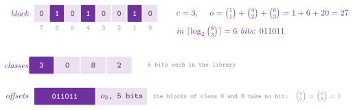
It cuts \(B\) in blocks of \(b = 63\) bits, and writes a block of \(c\) 1s as its
class \(c\), in 6 bits, and as its offset, its place among the
\(\binom{b}{c}\) blocks of class \(c\), in
\(\lceil \log_2 \binom{b}{c} \rceil\) bits. We compute the offset by the combinatorial number system.
Lemma 22.7 (the combinatorial number system). The vectors of \(b\) bits with \(c\) 1s at the places \(p_1 < \cdots < p_c\) are numbered from 0 to \(\binom{b}{c} - 1\) by
their rank in the colexicographic order. The place \(p\), scanned from \(b - 1\) down, holds the \(t\)-th 1, \(t\) being the 1s not yet met, if and only if \(\binom{p}{t} \le o\), where \(o\) is the remainder after the 1s above.
Proof. Note that the vectors that precede a given one in the colexicographic order are, for each \(t\), those that agree with it above \(p_t\) and have their \(t\) lowest 1s below \(p_t\), i.e., \(\binom{p_t}{t}\) of them, which gives (22.8). Since \(\sum_{t' < t} \binom{p_{t'}}{t'} < \binom{p_t}{t}\), the highest term of (22.8) is the largest \(\binom{p}{c} \le o\), which gives the decoding. \(\square\)
Theorem 22.1. RRRBitVector takes at most
\(m H_0( B ) + 0.175 m\) bits, with the rank in \(O( 32 + b )\) time and the
select in \(O( \log( m / 2016 ) + 32 + b )\) time.
Proof. Note that the product of the \(\binom{b}{c_j}\) of the blocks counts a part of the vectors of \(m\) bits with \(n\) 1s, and therefore by (22.2) \(\sum_j \log_2 \binom{b}{c_j} \le m H_0( B )\); the offsets, rounded up, take at most \(m H_0( B ) + m / b\) bits, and the classes \(6 m / b\). A superblock of 32 blocks (2016 bits) keeps the 1s before it and the place of its first offset, at most \(128 / 2016 = 6.3\%\) of \(m\). In all, one has \(m H_0( B ) + ( 7 / 63 + 128 / 2016 ) m < m H_0( B ) + 0.175 m\). As for the time, the rank of a place sums the classes of the blocks of its superblock before its own, and of their offsets the lengths, at most 31 of each, and rebuilds its block from the highest place down by Lemma 22.7, at most \(b\) steps. Similarly, the select finds the superblock by a binary search on the counts, the block by the classes, and the 1 in the rebuilt block. \(\square\)
Algorithm 22.8. The construction, the rank
and the select of RRRBitVector
(Raman, Raman and Rao 2007).
Note that a query walks only the places it needs: the rank stops at its place or at the last 1, the select at its bit. We write the walk with no branch, the binomials coming from a table of \(64 \times 64\) entries.
The function select0() does the same with the 0s of each block, counted as its length less its class. We rebuild the block in full when it is sparse in 0s.
22.6 Sequences of integers¶
In the representation of Elias 1974 and
Fano (chapters 11 and 15 of Ferragina 2023,
EliasFano.h) one codes a non-decreasing sequence
\(x_0 \le \cdots \le x_{n-1}\) of integers of \([ 0 , u )\) in about the bits
of the lower bound, and searches it in place.
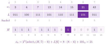
Theorem 22.2 (Elias and Fano). Let each \(x_i\) be split into its \(\ell = \lceil \log_2( u / n ) \rceil\) low bits, written in \(L\), and its bucket \(\lfloor x_i / 2^\ell \rfloor\), written by setting the bit
Then the sequence takes at most \(2 n + n \lceil \log_2( u / n ) \rceil\) bits, and \(x_i = 2^\ell ( \mathrm{select}_1( H , i + 1 ) - i ) + L[ i ]\).
Proof. Note that the places (22.9) are strictly increasing, since the buckets do not decrease and \(i\) grows, and therefore the \(( i + 1 )\)-th 1 of \(H\) is the one of \(x_i\), from which its bucket is read back by subtracting \(i\). Also, the 0s of \(H\) before that 1 are as many as the bucket, and hence \(H\) has \(n\) 1s. It has at most \(\lfloor ( u - 1 ) / 2^\ell \rfloor + 1 \le n\) 0s, since \(2^\ell \ge u / n\); \(L\) has \(n \ell\) bits. \(\square\)
Against the \(n \log_2( u / n ) + n \log_2 e\) bits of the lower bound, this
is less than 2 bits per item more when \(n\) is much smaller than \(u\)
(Figure 22.5). With the directory of
RankSelect on \(H\), access( i ) takes \(O( 1 )\) time, a select and a
field (Algorithm 22.9).
Algorithm 22.9. The construction, the access and the search of Elias-Fano.
The function nextGEQ( x ) gives the place of the first item \(\ge x\), which is the
rank of \(x\) (the items \(< x\)) and gives the predecessor and the successor.
Lemma 22.8. Let \(h = \lfloor x / 2^\ell \rfloor\). The first item \(\ge x\) is either in the bucket \(h\), whose items start after the \(h\)-th 0 of \(H\), or it is the first item of a later bucket; and among the items of the bucket \(h\) the low bits decide, since they are sorted.
Proof. The items of a bucket \(h' < h\) are below \(( h' + 1 ) 2^\ell \le h 2^\ell \le x\), and those of a bucket \(h' > h\) are at least \(( h + 1 ) 2^\ell > x\). Those of the bucket \(h\) share the high bits of \(x\), and they are compared with \(x\) by their low bits, which are in non-decreasing order within the bucket. Finally, the \(h\)-th 0 of \(H\) ends the bucket \(h - 1\), and the 1s after it, up to the next 0, are the items of the bucket \(h\). \(\square\)
Hence nextGEQ() costs a \(\mathrm{select}_0\) and a search of the low
bits of the bucket, and contains( x ) tests its result (\(\ell\) itself is
lowWidth()). The first 8 items of the bucket are scanned; past them,
which the clusters of a sequence may give, the end of the bucket is found
by \(\mathrm{select}_0\) too and its low bits by a binary search, so that a
bucket of \(c\) items costs \(O( 1 + \log c )\) steps beyond the selects. The
\(n\) items fall in \(\lceil u / 2^\ell \rceil\) buckets, at most \(n\) by the
proof of Theorem 22.2, and hence a bucket holds
at least one item on average.
Ferragina's book computes the rank by a binary search on the select, in
\(O( \log n )\) time; the bucket found by \(\mathrm{select}_0\) is the design
of the quasi-succinct indices of Vigna 2013
and of the sdarray of Okanohara and Sadakane 2007.
Viewed as the places of the 1s of a vector of \(u\) bits with \(n\) 1s, as in
chapter 15 of Ferragina, access( i ) is \(\mathrm{select}_1( i + 1 )\) of
that vector and nextGEQ( i ) is \(\mathrm{rank}_1( i )\), in
\(n ( 2 + \log( u / n ) ) + o( n )\) bits rather than \(u + o( u )\). We write
\(H\) with the 1s for the items and the 0s for the buckets, as in chapter 11
of Ferragina; its chapter 15 swaps them, which only swaps
\(\mathrm{select}_0\) and \(\mathrm{select}_1\). LazyEliasFano builds the
inventories of \(H\) at the first query that needs them, as LazyRankSelect
does.
Elias-Fano depends only on \(n\) and \(u\), and it ignores the "clusters" of a
sequence. In the partitioned form of Ottaviano and Venturini 2014
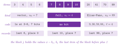
(PartitionedEliasFano) we cut a strictly increasing sequence into blocks of 128 items. We code the block \(j\), of \(m\) items, relative to \(b_j = x_{128 j - 1} + 1\), the end of the block before (0 for the first block). Its values \(v = x - b_j\) are in \([ 0 , u_j )\), with \(u_j\) the last of them plus 1, and the block is coded in the cheapest of three codes
(Figure 22.6). It takes no bit if \(u_j = m\) (all the values are there). It is a vector of \(u_j\) bits, the bit \(v\) for the value \(v\), if \(u_j\) is at most the bits of Elias-Fano. Otherwise it is Elias-Fano with \(\ell = \lfloor \log_2( u_j / m ) \rfloor\), in
\(m \ell + m + \lfloor ( u_j - 1 ) / 2^\ell \rfloor + 1\) bits. The function kinds()
counts the blocks of each of the three codes, and contains( x ) is a
nextGEQ() here too, as in LAVector.
Lemma 22.9. A block of \(m\) items with \(u > m\) costs at most \(\min\{ u , \, 2 m + m \lceil \log_2( u / m ) \rceil \}\) bits, i.e., never more than Elias-Fano with the \(\ell\) of Theorem 22.2 on its universe (with equality for \(u = m 2^\ell\)); hence the codes of all the blocks take at most
bits, at most one bit per item above the bound of Theorem 22.2 with the logarithm not rounded up.
Proof. Let \(\ell = \lfloor \log_2( u / m ) \rfloor\), the width of the code, so that \(m 2^\ell \le u < m 2^{\ell + 1}\). Its Elias-Fano form takes \(m \ell + m + \lfloor ( u - 1 ) / 2^\ell \rfloor + 1\) bits, and \(( u - 1 ) / 2^\ell < 2 m\) gives at most \(m \ell + 3 m\). If \(u / m\) is not a power of 2, \(\lceil \log_2( u / m ) \rceil = \ell + 1\) and this is \(2 m + m \lceil \log_2( u / m ) \rceil\). If \(u = m 2^\ell\), the term \(\lfloor ( u - 1 ) / 2^\ell \rfloor + 1\) is \(m\), and the cost is \(m \ell + 2 m = 2 m + m \log_2( u / m )\). The code taken is the cheapest of the vector of \(u\) bits and of this form (and no bit when \(u = m\)), which gives the first claim. For the sum, \(\lceil y \rceil < y + 1\) gives \(\sum_j m_j ( 3 + \log_2( u_j / m_j ) )\), and \(\sum_j u_j \le u\), since the universes of the blocks are disjoint ranges of \([ 0 , u )\); by the concavity of the logarithm (the inequality of Jensen on the weights \(m_j / n\)), \(\sum_j m_j \log_2( u_j / m_j ) \le n \log_2( \sum_j u_j / n ) \le n \log_2( u / n )\). \(\square\)
We remark that the extra bit per item of (22.10) comes from the rounding of the logarithm in each block, and it can be reached: on two blocks with \(u_1 / m = 1.5\) and \(u_2 / m = 2.5\) the ceilings sum to 3 per item, while the whole sequence, with \(u / n = 2\), has 1.
Besides, the records of the blocks cost a field of fixed width per block: the last item, the place of the code, and its kind with \(\ell\) in 8 bits (so that a query computes no logarithm). Also, the last item of each eighth block is kept apart for the searches. On the dense runs of an inverted index the cost is usually far smaller than that of Elias-Fano. The function access( i ) reads the
records of the block of \(i\) and of the one before (next to each other) and
selects the item in the code of the block, a scan of its few words. Also, nextGEQ( x ) finds the first block whose last item is at least \(x\) by a search of the items apart in the layout of Eytzinger (Khuong and Morin 2017), a complete binary tree by levels whose descent fetches the nodes three levels ahead. At most 8 records follow, and the item is found in its block by the high
part, or by the sideways sums of the vector up to \(x\)
(Algorithm 22.10). Ottaviano and Venturini also
choose the ends of the blocks by an approximate dynamic program on the cost
of the codes, which gains a further 10% or so on the lists of an index; the
blocks here have the fixed size of their uniform partition.
Algorithm 22.10. The construction, the access and the search of the partitioned Elias-Fano (Ottaviano and Venturini 2014).
Elias-Fano spends on each item the same bits, whatever the regularity of
the gaps. In the LA-vector of Boffa, Ferragina and Vinciguerra 2021 (LAVector) one spends them instead on
the distance of each item from a line. We cover the points \(( i , x_i )\) by the fewest segments whose lines are within \(\epsilon\) of each of their
points, the optimal piecewise linear approximation of the PGM-index
(Ferragina and Vinciguerra 2020,
ADS/search/PGMIndex.h), and each item is stored as its correction with
respect to the line of its segment (Figure 22.7).
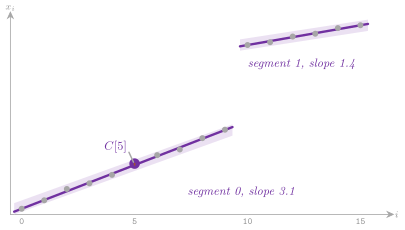
Lemma 22.10 (the corrections). Let the segment \(j\), over the places \([ p_j , p_{j+1} )\), have a line \(f( i ) = x_{p_j} + \gamma + \alpha ( i - p_j )\) with \(| f( i ) - x_i | \le \epsilon\) for each of its places, and let \(d_i = x_i - x_{p_j} - \lfloor \alpha ( i - p_j ) \rfloor\). Then the \(d_i\) take at most \(2 \epsilon + 2\) values, and with \(\beta_j = x_{p_j} + \min_i d_i\)
Proof. \(x_i - x_{p_j} - \alpha ( i - p_j )\) lies in \([ \gamma - \epsilon , \gamma + \epsilon ]\), and taking off the integer part of \(\alpha ( i - p_j )\) instead of the whole of it adds less than 1. Hence the \(d_i\) are integers in an interval of length less than \(2 \epsilon + 2\), at most \(2 \epsilon + 2 = 2^c\) of them, and \(C[ i ] = d_i - \min_i d_i\) takes \(c\) bits. \(\square\)
In the code the slope \(\alpha\) is kept in a double, whose rounding may spread the
\(d_i\) by a few units on items of 64 bits. LAVector therefore computes the
corrections with the rounded slope and gives each segment the width \(w_j\)
of the range of the corrections of the segment, so that (22.11) holds with \(w_j\) in
place of \(c\) (\(c\), or one bit more). One can count the space as follows. A segment takes 24 bytes (the base, the slope, and the place of its corrections with their width; its first item is its base plus its first correction). Its first place takes a field of \(\lceil \log_2 n \rceil\) bits, and the two tables that find a segment by a place and by a value about two fields of \(\lceil \log_2 m \rceil\) bits per segment. Hence the sequence takes about
bits for \(m\) segments (Algorithm 22.11).
Algorithm 22.11. The construction, the access and the search of the LA-vector (Boffa, Ferragina and Vinciguerra 2021), and the choice of the width of the corrections.
Accessing \(x_i\) is (22.11) once the segment of \(i\) is known, which a table of the segment of each \(2^t\)-th place gives after a scan of the segments that start among the \(2^t\) places before \(i\), one on average for \(2^t \approx n / m\). In turn, the rank of \(x\) first finds the last segment whose first item is below \(x\), through a table of the first segment of each bucket of the high bits of the items, as the buckets of Elias-Fano. Then, since by (22.11) \(\beta_j + \lfloor \alpha ( i - p_j ) \rfloor \le x_i < \beta_j + \lfloor \alpha ( i - p_j ) \rfloor + 2^{w_j}\), the answer is among the places where the line goes from \(x - 2^{w_j}\) to \(x + 1\), about \(2^{w_j} / \alpha\) of them. A binary search on the corrections settles it in \(O( w_j - \log_2 \alpha )\) steps; when the floating point misplaces the window, which the search checks on the two items at its ends, the whole segment is searched.
Against Elias-Fano, which takes \(2 + \lceil \log_2( u / n ) \rceil\) bits per item, the LA-vector may win when the items follow lines "closely". This happens, e.g., on the places of a pattern repeated with some noise, on the keys of a process that grows at a steady rate, or on the dense runs of an inverted index, where \(m\) is small and \(c\) is the logarithm of the noise instead of the average gap. On gaps drawn at random no line may follow the items better than the average gap does, the corrections need about \(\log_2( u / n )\) bits as
the low bits of Elias-Fano, and the segments are an overhead. The function tuned()
therefore tries the widths up to six bits above the logarithm of the
average gap (or half the bits of the items, if more) and keeps the one of
the fewest bits. In the journal form of Boffa, Ferragina and Vinciguerra 2022, the LA-vector chooses the width segment by segment, by a shortest path over the segments
of all the widths. Its gain comes from segments of different widths, which the width \(w_j\)
that each segment takes from its corrections already gives in part, and
the library does not implement the shortest path.
22.7 Arrays of packed fields¶
An array of \(n\) values below \(2^B\) takes \(n B\) bits when its fields are
packed in words, against the \(8 n\) of a byte per value. In the searches, the tables of "large" spaces of states may have \(10^9\) entries and more, e.g., the pattern databases of the heuristic search (Felner, Korf and Hanan 2004), and they fit in the memory only so packed.
PackedArray< B > takes the widths that divide 64, \(B \in \{ 1 , 2 , 4 , 8 , 16 , 32 \}\). A word then holds \(64 / B\) fields (the constant PER, and MAX is \(2^B - 1\), the largest value of a field), and the field \(i\) is the bits \(( i \bmod 64 / B ) B\) on of the word \(\lfloor i B / 64 \rfloor\). A read is one load, one shift and one mask, with no test of a field that crosses two words, which BitVector::get( i , len ) pays for the other widths
(Figure 22.8). A write clears the field by a mask
and puts the value by an or, in the same word.
A saturated array (the template parameter Saturate) stores a value
above \(2^B - 1\) as \(2^B - 1\), and counts it in clamped(), instead of
breaking the contract. When the values are lower bounds, e.g., the
distances of a pattern database, a value cut down is still a "good" lower bound,
and \(B\) is then chosen for most of the values rather than for the largest
one.
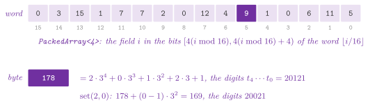
A value of three states carries \(\log_2 3 \approx 1.585\) bits of
information, but takes 2 bits in a field of PackedArray< 2 >. We may put five such values (trits) \(t_0 , \ldots , t_4\) in one byte as the number
i.e., in 1.6 bits per value, 0.015 above the entropy and one fifth less than the fields of 2 bits (Breyer and Korf 2010, whose tables keep the distances modulo 3, from which the distance of a state is recovered along a path to the goal). TritArray reads the digit \(j = i \bmod 5\) of the byte \(\lfloor i / 5 \rfloor\) from a table of the five digits of each of the 243 bytes, 1215 bytes that stay in the cache of the first level. It writes the digit by adding \(( v - t_j ) 3^j\) to the byte, which by
(22.13) changes only that digit.
Six values would need \(3^6 = 729 > 256\) codes, and \(3^{40} < 2^{64} < 3^{41}\) would put 40 values in a word, 1.6 bits each again, at the price of a division by a power of 3 per read; the byte is the unit with the same density and a read by a table. Both arrays are also built from a function \(f\) of the place by blocks of whole words (of whole bytes for the trits) on the threads of an executor (Algorithm 22.12). A word is written by the one thread that owns its block, and therefore no write needs an atomic and the array is the same as the sequential one; the work is \(O( n )\) calls of \(f\), with the depth of one block.
Algorithm 22.12. The parallel construction
and the write of PackedArray and of TritArray.
22.8 Trees¶
One can code a tree by its shape and nothing more, in about the \(2 n\) bits of the lower bound of §22.1, and its nodes are then numbered by the places of their bits; the data of a node go in a vector indexed by its number. We give three codes, which differ in the operations that they answer in constant time.
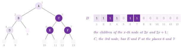
Lemma 22.11 (the binary tree of Jacobson). Complete a binary tree of \(n\) nodes with a leaf in place of each missing child, and write by levels a 1 for a node and a 0 for a leaf added, in \(B[ 1 , 2 n + 1 ]\). Then the children of the \(x\)-th node are at the places \(2 x\) and \(2 x + 1\), and the item at the place \(p\) is the \(\mathrm{Rank}_1( p )\)-th node if \(B[ p ] = 1\).
Proof. A visit by levels lists the root at the place 1, and then the children of the nodes in the order of the nodes, two per node. Hence the children of the first \(x - 1\) nodes take the places \(2 , \ldots , 2 x - 1\), and those of the \(x\)-th one the next two. \(\square\)
One can see that, with rank and select in \(O( 1 )\) time, the left child of
the \(x\)-th node is the \(\mathrm{Rank}_1( 2 x )\)-th node, if \(B[ 2 x ] = 1\),
and its parent the \(\lfloor \mathrm{Select}_1( x ) / 2 \rfloor\)-th; in the
notation of Ferragina's book, which names a node by its place \(p\), the left
child is at the place \(2 \, \mathrm{Rank}_1( p )\) and the parent at
\(\mathrm{Select}_1( \lfloor p / 2 \rfloor )\). Hence JacobsonTree
(Jacobson 1989) takes
\(2 n + 1 + o( n )\) bits, within \(O( \log n )\) of the lower bound, with
left(), right() and parent() in \(O( 1 )\) time
(Figure 22.9). In the library the nodes are numbered \(0 , \ldots , n - 1\) by levels and
the places from 0, i.e., the node \(v\) is the \(( v + 1 )\)-th node and the
place \(q\) is the place \(q + 1\) of Lemma 22.11. Then the node \(v\) is at the
place \(\mathrm{select}_1( v + 1 )\); its left child is at the place \(2 ( v
+ 1 ) - 1 = 2 v + 1\), and it is the node \(\mathrm{rank}_1( 2 v + 1 )\) if
that place holds a 1; and its parent is the \(\lfloor ( \mathrm{select}_1(
v + 1 ) + 1 ) / 2 \rfloor\)-th node, i.e., the node \(\lfloor (
\mathrm{select}_1( v + 1 ) + 1 ) / 2 \rfloor - 1\)
(Algorithm 22.13). This representation answers
the navigation, but not the size of a subtree, which needs the order of a
visit in depth.
Algorithm 22.13. The code by levels of a binary tree, and its left child and parent (Jacobson 1989).
For a tree of any degree, LOUDS (the level-order unary degree sequence of
Jacobson, LoudsTree) puts a dummy root of degree 1 above the root and
writes the degree \(d\) of each node, by levels, as \(0^d 1\). Hence the code has \(n\) 0s, one per node (each node is the child of somebody), and \(n + 1\) 1s,
one per node and the dummy root, i.e., \(2 n + 1\) bits
(Figure 22.10).
Lemma 22.12. In the code of LOUDS, the \(k\)-th 0 is the \(k\)-th node by levels, and the children of the \(k\)-th node are the 0s after the \(( k + 1 )\)-th 1. Hence, with the nodes numbered from 0 and the places from 0,
the latter when a 0 follows the \(( v + 1 )\)-th 1, and \(\mathrm{degree}( v ) = \mathrm{select}_1( v + 2 ) - \mathrm{select}_1( v + 1 ) - 1\).
Proof. Each node writes a 0 for each of its children, in the order by levels. These 0s come in the order of the nodes that they stand for, since the visit by levels lists the children of the nodes in the order of the nodes, and the dummy root writes the 0 of the root. Furthermore, the \(( k + 1 )\)-th 1 ends the unary degree of the \(k\)-th node (the first 1 being that of the dummy root), and its children are the 0s that follow it. In particular, the 0 of \(v\) is at \(q = \mathrm{select}_0( v + 1 )\), and the 1s before it are \(q - v\), of which the first is the dummy root's; hence its parent is the node \(q - v - 1\). Similarly, the 0 after the \(( v + 1 )\)-th 1, at \(p + 1\) with \(p = \mathrm{select}_1( v + 1 )\), is the \(( p + 1 - v )\)-th 0, i.e., the node \(p - v\). \(\square\)
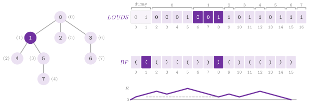
Its functions are leftmostChild() and rightSibling(), the names of the
TREE of the book (ADS/tree/Tree.h); the \(i\)-th child is the first one
plus \(i\), since the children of a node are consecutive in the order by
levels, which a visit in depth does not give (Algorithm 22.14).
LOUDS does not answer the size of a subtree nor the depth of a node; it is the simplest of the succinct trees and, arguably, the "fastest" for the
navigation from the root down
(Arroyuelo, Cánovas, Navarro and Sadakane 2010),
e.g., in the tries of the indices.
Algorithm 22.14. The code by LOUDS of an ordered tree.
In turn, the balanced parentheses (BPTree, after
Munro and Raman 2001) write an open
parenthesis, a 1, when a visit in depth enters a node, and a closed one, a
0, when it leaves it. Hence the nodes of a subtree are consecutive in preorder, and a node is the pair of its parentheses. With the excess
\(E( i )\), the open parentheses less the closed ones in \(B[ 0 , i ]\) (and
\(E( -1 ) = 0\)), one has
(cf. Figure 22.10), and similarly for
findOpen() and enclose(), the open parenthesis of the pair that
encloses the one at \(i\).
Lemma 22.13. In a balanced sequence of
parentheses, (i) (22.15) gives the closed parenthesis that matches the open
one at \(i\); (ii) findOpen( j ) is \(k + 1\) for the last \(k < j\) with \(E( k
) = E( j )\), and enclose( i ) is \(k + 1\) for the last \(k < i\) with \(E( k
) = E( i ) - 2\); (iii) the first place after (or before) a start whose
excess is at most a target \(t\) below the excess of the start has the
excess \(t\); (iv) \(E( i ) = 2 \, \mathrm{rank}_1( i + 1 ) - ( i + 1 )\).
Proof. (iv) Among the \(i + 1\) parentheses of \(B[ 0 , i ]\), the open ones are \(\mathrm{rank}_1( i + 1 )\) and the closed ones the rest. (iii) The excess changes by \(\pm 1\) from a place to the next, and therefore it cannot pass from above \(t\) to below \(t\) without taking the value \(t\). (i) The parenthesis at \(i\) is open, so that \(E( i ) = E( i - 1 ) + 1\). The parentheses strictly inside its pair form a balanced sequence, whose prefixes have a nonnegative excess, and hence \(E( j ) \ge E( i )\) inside the pair; the matching closed parenthesis at \(c\) gives \(E( c ) = E( i ) - 1\), and \(c\) is therefore the least \(j > i\) with that excess. (ii) For the closed parenthesis at \(j\) and its match at \(o\), the parentheses between them are balanced, so that \(E( o - 1 ) = E( j )\) and \(E( k ) > E( j )\) for \(o \le k < j\); hence \(o - 1\) is the last \(k < j\) with \(E( k ) = E( j )\). The pair that encloses the one at \(i\) opens at the last place \(o' < i\) whose parenthesis is open and whose pair contains \(i\). Between \(o'\) and \(i\) the parentheses are balanced pairs, so that \(E( i - 1 ) = E( o' )\), i.e., \(E( o' - 1 ) = E( i ) - 2\), and each \(k\) with \(o' \le k < i\) has \(E( k ) \ge E( i ) - 1\). \(\square\)
By (iii), each operation is a search for the first place, forward or backward, whose excess reaches a target, and by (iv) the excess of a place costs \(O( 1 )\) time.
BalancedParentheses answers the searches by the range min-max tree of
Navarro and Sadakane 2014. It keeps,
for each leaf of 512 bits, for each group of 16 leaves and for each node of
a complete binary tree over the groups, the total excess of its range and
its minimum prefix excess. A search runs on the excess relative to its
start, and needs no rank. It scans the leaf of \(i\) a byte at a time, with the excess, the minimum and the place of each target of each of the 256 bytes in tables. Then it scans the leaves of the group of \(i\) by their excess and minimum in 16 bits. At last it climbs the tree, whose leaves are the groups, to the first range on its side whose minimum reaches the target, and goes down to its group, its leaf and its byte
(Algorithm 22.15). A range whose minimum stays above the target holds no answer, by (iii) of
Lemma 22.13, and it is skipped whole; the
first range on the side of the search whose minimum reaches the target
holds the answer, again by (iii). The search thus scans at most two leaves
of \(512 / 8\) bytes, two groups of 16 leaves, and climbs and descends the
binary tree over the \(n / 8192\) groups, i.e., \(O( \log( n / 8192 ) + 16 +
512 / 8 )\) time. In a tree, most searches end in the leaf of \(i\), at the
cost of one miss of the cache.
Algorithm 22.15. The range min-max tree, and
the forward search of findClose()
(Navarro and Sadakane 2014).
In space, the tree takes \(32 / 512\) bits per parenthesis for the leaves (6.25%) and
at most \(4 \cdot 128 / 8192\) for the groups, besides the directory of rank
of CompactRankSelect, 3.5% of the bits, since no search needs a rank.
The function forwardSearch( i , d ) gives the first \(j > i\) with \(E( j ) - E( i ) = d < 0\). This may also be the end of a subtree of the code
by the degrees in depth (ADS/dictionary/SuccinctPatriciaTrie.h).
Jacobson 1989 gives findClose() in
\(O( \log n )\) time with the pioneers, and Munro and Raman in \(O( 1 )\) time
with two levels of pioneers and tables, in \(2 n + o( n )\) bits. Then the range min-max tree of Navarro and Sadakane reaches \(O( 1 )\) time with a tree of degree \(\Theta( \log n )\) and tables. Its binary form with blocks of a few
hundred bits, the one here, is usually the fastest in practice, at least on the trees of the benchmarks
(Arroyuelo, Cánovas, Navarro and Sadakane 2010;
Gog and Petri 2014;
Grossi and Ottaviano 2013).
BPTree numbers the nodes in preorder, the node \(v\) being the
\(( v + 1 )\)-th open parenthesis. The function parent( v ) is enclose() of its open
parenthesis, leftmostChild( v ) is \(v + 1\) if the next parenthesis is an
open one, and rightSibling( v ) is the open parenthesis after its closed
one, if any (Algorithm 22.16). Furthermore,
subtreeSize( v ) is \(( j - i + 1 ) / 2\) for its parentheses at \(i\) and
\(j\), depth( v ) is the excess at its open parenthesis less 1, and \(u\) is
an ancestor of \(v\) if \(u \le v < u + \mathrm{subtreeSize}( u )\), the test
of isAncestor( u , v ). These may cost a search of the range min-max tree, or a select and a rank for
leftmostChild(), depth() and isLeaf().
Lemma 22.14. With the node \(v\) at the
open parenthesis \(i\) and its match at \(j\), the subtree of \(v\) has \(( j - i +
1 ) / 2\) nodes, numbered \(v , \ldots , v + ( j - i - 1 ) / 2\) in preorder,
the depth of \(v\) is \(E( i ) - 1\), and the formulas of parent(),
leftmostChild(), rightSibling() and isAncestor() above are right.
Proof. The visit in depth writes the parentheses of the subtree of \(v\) between entering and leaving \(v\), i.e., in \(B[ i , j ]\), two per node, and it enters these nodes consecutively in preorder, starting from \(v\). The open parentheses before \(i\) whose match is after \(i\) are those of the ancestors of \(v\), and the others before \(i\) are matched before it; hence \(E( i - 1 )\) is the number of the proper ancestors of \(v\), which is its depth, and \(E( i ) - 1 = E( i - 1 )\). The parent of \(v\) is the nearest of these ancestors, the pair that encloses \(i\) (Lemma 22.13); the first child of \(v\), if any, is entered right after \(v\), at \(i + 1\), and it is the node \(v + 1\); the next sibling of \(v\), if any, is entered right after leaving \(v\), at \(j + 1\). Finally, \(u\) is an ancestor of \(v\) (or \(v\) itself) if and only if \(v\) is in the subtree of \(u\), i.e., \(u \le v < u + \mathrm{subtreeSize}( u )\). \(\square\) Against LOUDS, the parentheses give the size of a subtree, the depth and the ancestors, and number the nodes of a subtree consecutively (from \(v\) to \(v + \mathrm{subtreeSize}( v ) - 1\)), at the price of the searches. We remark that DFUDS of Benoit et al. 2005, the degrees in unary in preorder, also gives the \(i\)-th child in \(O( 1 )\) time with the same matching; chapter 15 of Ferragina does not treat it, and neither does the library.
Algorithm 22.16. The parentheses of a tree
by a visit in depth, and the parent and the next sibling in BPTree.
Table 22.3 compares the trees, and the graphs of §22.10.
Table 22.3. The trees and the graphs and their costs, for \(n\) nodes and \(m\) edges.
| Realization | Space in bits | Operations |
|---|---|---|
JacobsonTree |
\(2 n + 1 + o( n )\) | the children and the parent of a binary tree in \(O( 1 )\) |
LoudsTree |
\(2 n + 1 + o( n )\) | the parent, the degree, the \(i\)-th child and the next sibling in \(O( 1 )\) |
BPTree, on BalancedParentheses |
\(2 n\), and 6.25% of them for the leaves of the range min-max tree, at most as much for its groups and 3.5% for a rank directory | also the size of a subtree, the depth and the ancestors, by a search of the excess |
EliasFanoGraph |
\(m ( 2 + \lceil \log_2( n^2 / m ) \rceil ) + n ( 2 + \lceil \log_2( m / n ) \rceil )\) | the outdegree and the \(i\)-th successor in \(O( 1 )\), an edge by a nextGEQ() |
BVGraph |
about 3 per edge on the Web graphs | a list in \(O( R d )\), \(R\) the longest chain of references |
K2Tree |
\(k^2 m ( \log_{k^2}( n^2 / m ) + O( 1 ) )\) in the worst case | an edge in \(O( h )\), the successors and the predecessors of a node |
22.9 Sequences of symbols and permutations¶
Our wavelet matrix, that of Claude, Navarro and Ordóñez 2015
(WaveletMatrix), holds a static sequence \(S[ 0 .. n - 1 ]\) of integers of
\(w\) bits in \(n w\) bits plus the directories of rank and select, with the
access, the rank and the select of any symbol in \(O( w )\) time.
Lemma 22.15 (the wavelet matrix). Let the level \(\ell\) of \(S\) hold the bit \(w - 1 - \ell\) of each item, the items passing to the next level stably sorted by that bit, the \(Z_\ell\) with a 0 first. Then the item at the place \(i\) of a level is at the place
of the next one, and the items equal to \(c\) end consecutive, in the order of \(S\), at the last level.
Proof. A stable partition by a bit sends an item to the place given by the items with its bit before it, which is (22.16), and keeps the order among the items with the same bit. By induction on the levels, the items that share the first \(\ell\) bits stay consecutive, in the order of \(S\). Also, the place of the range of \(c\) at the last level depends on the bits of \(c\) alone. \(\square\)
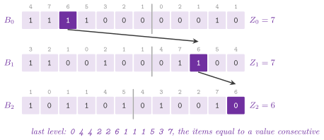
Hence access(), rank() and select() follow a place, or the two ends of
a range, down the \(w\) levels by (22.16), or up by the select, in \(O( w )\)
time (Figure 22.11); rank( c , i ) follows
the places 0 and \(i\) down along the bits of \(c\), and the difference at the
last level is the answer.
Furthermore, the \(k\)-th smallest item of a range, quantile( i , j , k ), goes down to
the 0s or to the 1s according to how many 0s the range holds at each level,
and countLess( i , j , c ) sums the 0s that the range leaves at the levels
where \(c\) has a 1 (Algorithm 22.17). Instead, the wavelet tree of Grossi, Gupta and Vitter 2003 splits the alphabet in halves at its nodes, which need a pointer or an offset each. Our matrix keeps instead one vector of \(n\) bits per level and no tree, at the same costs, and it is arguably the form of choice for the large alphabets, and the base
of the compressed indices of the integers (Navarro 2014
surveys the uses of the wavelet trees). Each level carries the directory of
RankSelect, and the matrix therefore takes about \(1.5 \, n w\) bits, a
query of rank being \(2 w\) ranks of one load and one sideways sum each.
Algorithm 22.17. The access, the rank, the select, the quantile and the count of the wavelet matrix (Claude, Navarro and Ordóñez 2015).
Lemma 22.16. For \(0 \le i < j \le n\)
and \(k < j - i\), quantile( i , j , k ) returns the \(k\)-th smallest item
of \(S[ i .. j - 1 ]\), from 0, and countLess( i , j , c ) the number of
its items smaller than \(c\), each with \(2 w\) ranks.
Proof. By Lemma 22.15, before the level \(\ell\) the range \([ i , j )\) holds exactly the items of the original range whose first \(\ell\) bits are those chosen so far, the prefix \(c\) of the result. Line 4 computes the number \(z\) of those whose next bit is 0, which by (22.16) go to the range \([ i - i_1 , j - j_1 )\) of the next level, the others to \([ Z_\ell + i_1 , Z_\ell + j_1 )\). For the quantile, we keep the invariant that the answer is the \(k\)-th smallest item of the current range: all the items with the next bit 0 are smaller than those with the bit 1 and the same prefix, so that the answer has the bit 0 if and only if \(k < z\), and otherwise it is the \(( k - z )\)-th of the items with the bit 1. After \(w\) levels the prefix is the whole item. For the count, an item of the range is smaller than \(c\) if and only if, at the first bit where they differ, the item has 0 and \(c\) has 1. At a level where \(c\) has the bit 1, line 6 counts the items of the range with the bit 0, which agree with \(c\) on the bits before and are smaller, and follows those with the bit 1; where \(c\) has 0, the items with the bit 1 are larger and are dropped. The items equal to \(c\) are not counted. Each level costs two ranks. \(\square\)
A wavelet tree shaped by the code of Huffman
(Mäkinen and Navarro 2005,
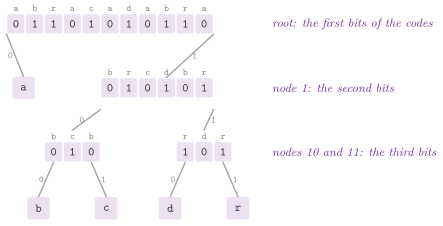
HuffmanWaveletTree) takes \(n ( H_0 + 1 )\) bits instead of \(n w\), and it may be somewhat faster on a "skewed" alphabet, quite often the case of a text. We give the symbol \(c\) the canonical code of Huffman of its frequency, of length \(\ell_c\) (codeLength( c ), 0 for a symbol absent), with its bits from the highest. Our tree is the trie of the codes, and its internal node \(v\),
reached by the prefix \(\pi_v\), keeps the bit after \(\pi_v\) of the code of
each item whose code starts with \(\pi_v\), in the order of the sequence
(Figure 22.12). We give the canonical codes by length and then by symbol, the first one 0, which is another convention than
(21.5) of §21.2, with the same lengths. All the nodes have their bits in one vector \(B\) with rank and select, the node \(v\)
from the place \(o_v\), with \(R_v = \mathrm{rank}_1( B , o_v )\) kept. An
item of place \(i\) in the node \(v\) moves to the place
of its child by the bit \(b = B[ o_v + i ]\). A descent along the code of \(c\) gives access( i ), together with the rank of the symbol found (accessRank(), the LF-mapping of an FM-index in one descent). It also gives \(\mathrm{rank}_c( i )\), one rank a step, while \(\mathrm{select}_c( k )\)
climbs from the leaf of \(c\) by one select a step,
\(k' = \mathrm{select}_b( B , \mathrm{rank}_b( B , o_v ) + k ) - o_v + 1\)
(Algorithm 22.18).
Lemma 22.17. The bits of the nodes of
HuffmanWaveletTree are \(\sum_c f_c \ell_c < n ( H_0 + 1 )\), for the
frequencies \(f_c\) of the symbols.
Proof. An item of the symbol \(c\) leaves one bit in each of the \(\ell_c\) internal nodes on the code of \(c\). Hence the sum is \(n\) times the average length of the code of Huffman of the frequencies, which is below \(H_0 + 1\) by (21.4). \(\square\)
Beside the bits of \(B\), the tree takes the directory of rank and select,
25% of them with RankSelect and 3.5% with CompactRankSelect (the
template parameter RS, time against bits), and \(O( \sigma )\) words of the
nodes and of the codes. With withSelect false, the directory of RankSelect builds no inventory. This suits a tree that only ranks, such as the one of the FM-index of §21.11.
Algorithm 22.18. The construction, the access with the rank, the rank and the select of the wavelet tree of Huffman (Mäkinen and Navarro 2005).
Finally, the move structure of Nishimoto and Tabei 2021
(MoveStructure) represents a permutation \(\pi\) of \([ 0 , n )\) that
shifts each of \(r\) intervals \([ p_i , p_{i+1} )\) alike, such as the
LF-mapping of a transform of Burrows and Wheeler on its runs, or the
function \(\phi\) of the r-index (§21.11). It
keeps the starts \(p_i\), their images \(q_i\) and the interval \(d_i\) that holds
\(q_i\), so that
and the interval of \(\pi( x )\) is found from \(d_i\) forward, past the starts \(p_j \le \pi( x )\).
We say that the structure is balanced when no image \([ q_i , q_i + p_{i+1} - p_i )\) holds 4 starts or more. Its construction ensures it by cutting an interval whose image holds 4 starts at the third of them, so that the first part holds 2; the new start may weigh on another image (the cut may cascade), which is checked in turn (Algorithm 22.19). Then the intervals become at most \(2 r\) (Nishimoto and Tabei, for this balance), and the search forward takes at most 3 steps (Lemma 22.18 below); hence each step of a walk costs \(O( 1 )\) time, in \(O( r )\) words instead of the \(n\) of the permutation written in full. On the runs of the transform of abracadabra (cf. Table 21.7) the image of the run of a, the rows \([ 6 , 10 )\), is the rows \([ 2 , 6 )\), which hold the 4 starts 2, 3, 4 and 5; the balance cuts the run at the row 8 (Figure 22.13). We keep the intervals and the images in two ordered maps during the construction, \(O( r \log r )\) time, and each interval carries a tag (the symbol of its run), which its parts keep.
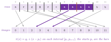
Algorithm 22.19. The balance and the move of Nishimoto and Tabei 2021.
Lemma 22.18. If the structure is
balanced, move( x , i ) with \(x \in [ p_i , p_{i+1} )\) returns \(\pi( x
)\) and the interval that holds it after at most 3 iterations of line 3.
Proof. By (22.18), \(y = \pi( x )\) lies in the image \([ q_i , q_i + p_{i+1} - p_i )\), which starts in the interval \(d_i\). The loop moves \(j\) forward while the next start is at most \(y\), and stops at the interval that holds \(y\). Each start that it passes lies in \(( q_i , y ]\), inside the image, which holds at most 3 starts by the balance. \(\square\)
The bound of \(2 r\) on the intervals after the balance is the theorem of Nishimoto and Tabei 2021 for the cut of an image of 4 starts, which the construction of the library follows.
Table 22.4 summarizes the sequences of the area.
Table 22.4. The sequences and their costs.
| Realization | Space in bits | Access | Search |
|---|---|---|---|
EliasFano |
\(n ( 2 + \lceil \log_2( u / n ) \rceil )\), plus the directory of \(H\) | \(O( 1 )\) | nextGEQ() in a \(\mathrm{select}_0\) and \(O( 1 + \log c )\) for a bucket of \(c\) items |
PartitionedEliasFano |
at most that of Elias-Fano on each block of 128 items, plus a record per block | a scan of the code of a block | nextGEQ() by a search of the records and the scan of a block |
LAVector |
(22.12) | a lookup and a scan of the segments of \(2^t\) places | nextGEQ() in \(O( w_j - \log_2 \alpha )\) once the segment is found |
WaveletMatrix |
\(n w\), plus a directory per level | \(O( w )\) | rank, select, quantile and range counts in \(O( w )\) |
HuffmanWaveletTree |
less than \(n ( H_0 + 1 )\), plus the directory and \(O( \sigma )\) words | \(O( \ell_c )\), \(H_0 + 1\) on average | rank and select of \(c\) in \(O( \ell_c )\) |
MoveStructure |
\(O( r )\) words for a permutation of \(r\) intervals | the image of a place and its interval in \(O( 1 )\) | the interval of a place by a binary search |
22.10 Graphs¶
A graph of \(n\) nodes and \(m\) edges, as sorted adjacency lists, is a set of
\(m\) pairs among \(n^2\), i.e., \(\log_2 \binom{n^2}{m} \approx
m \log_2( n^2 / m )\) bits for a graph with no regularity.
EliasFanoGraph writes the edge \(( u , v )\) as the integer \(u n + v\). Its lists, each one sorted, are then one increasing sequence of \([ 0 , n^2 )\) coded by Theorem 22.2, and a second sequence of the prefix sums of the outdegrees gives where each list starts (Figure 22.14). This is the
representation of the adjacency lists of large graphs in Unicorn
(Curtiss et al. 2013) and in the
quasi-succinct indices of Vigna 2013.
Hence the outdegree and the \(i\)-th successor are accesses, in \(O( 1 )\)
time, and an edge \(( u , v )\) is the test of nextGEQ( u n + v )
(Algorithm 22.20).
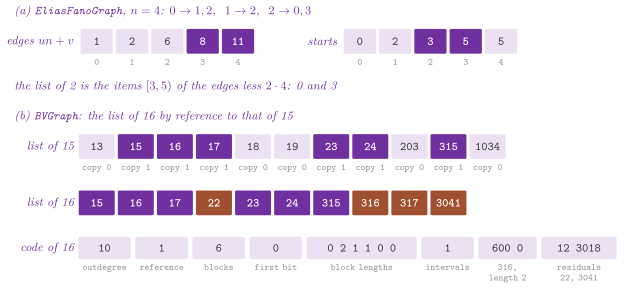
Algorithm 22.20. The construction of the graph in Elias-Fano.
Lemma 22.19. Coding each list apart, in the universe of the list, takes
bits beyond the \(2 m\) of the unary parts, \(d_u\) being the outdegree of \(u\).
Proof. By the concavity of the logarithm (the inequality of Jensen on the weights \(d_u / m\)), \(\sum_u ( d_u / m ) \log_2( n / d_u ) \le \log_2( \sum_u ( d_u / m ) ( n / d_u ) ) = \log_2( n^2 / m )\), the sum running over the \(u\) with \(d_u > 0\), which are at most \(n\). \(\square\)
Coded apart, the lists can thus take fewer bits when the degrees are skewed, at
the price of a directory and an offset per list, the form that chapter 15
of Ferragina describes; the single sequence keeps one directory and the
same \(O( 1 )\) access. Neither exploits the locality and the similarity of
the lists of the Web, which the codes of
Boldi and Vigna 2004 do. With the pages
sorted by URL, most links stay in the host (locality), and the pages of a
host link to the same pages (similarity). BVGraph codes the list of \(x\) as its outdegree, in \(\gamma\), followed by the reference \(r\): the list of \(x - r\), among the previous \(W\) lists, that shares the most successors with that of \(x\) (0 for none). Then comes the copy list of the reference, a bit per successor of \(x - r\) that records whether it is a successor of \(x\) too. It is written as copy blocks, i.e., its first bit and the lengths less 1 of its runs, the last one omitted since the outdegree of the reference implies it. Next come the successors not copied, the extra nodes. These are the runs of at least \(L_{\min}\) consecutive integers as intervals (each an Interval, its
left extreme and its length), and the residuals as
gaps less 1, the first ones of each relative to \(x\) by signedToNatural()
(Algorithm 22.21).
Algorithm 22.21. The coding and the
decoding of a list of BVGraph, and two of its steps
(Boldi and Vigna 2004).
A list is decoded from its place in the stream, kept for each node in an
Elias-Fano sequence, after the list of its reference. Since the chains of references are at most \(R\) long, a list is decoded in \(O( R d )\) time for outdegrees up to \(d\). With the window \(W = 7\), the
chains \(R = 3\) and \(L_{\min} = 4\) (the defaults of the WebGraph framework),
the Web graphs usually take about 3 bits per edge, as Boldi and Vigna measure,
against the \(\log_2 n\) bits of a plain list and the
\(2 + \log_2( n^2 / m )\) of Elias-Fano. Also, the WebGraph framework codes the gaps
by the \(\zeta\) codes, tuned to their power-law distribution, and reorders
the nodes (e.g., by the layered label propagation of
Boldi et al. 2011) to make the locality
stronger; neither is in chapter 15 of Ferragina, nor in the library.
The functions copyList(), copyBlocks(), intervals() and residualGaps() are the
steps of the coding, given for the examples of that chapter.
The \(k^2\)-tree of Brisaboa, Ladra and Navarro 2014 (K2Tree) splits the adjacency matrix, padded to the side \(N = k^h \ge n\), into \(k^2\) submatrices of side \(N / k\). Each one is a child of the root, marked 1 if it has an edge and 0 otherwise, and each child marked 1 is split again, down to the cells. We write the marks by levels: \(T\) has those of all
the levels but the last, and \(L\) those of the cells
(Figure 22.15).
Lemma 22.20. The children of the node marked at the place \(p\) of \(T\) start at the place \(k^2 \, \mathrm{rank}_1( T , p + 1 )\) of \(T\) followed by \(L\).
Proof. Recall that the marks are written by levels, the \(k^2\) children of each node marked 1 in the order of the marks. Thus the children of the root take the places \(0 , \ldots , k^2 - 1\), and those of the \(j\)-th mark 1 of \(T\) come after the children of the root and of the \(j - 1\) marks 1 before it, i.e., they start at \(k^2 j\), with \(j = \mathrm{rank}_1( T , p + 1 )\). \(\square\)
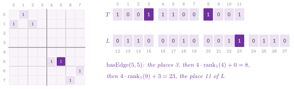
Hence no pointer is stored, as in LOUDS, and one can walk the tree by ranks only. The function hasEdge( u , v ) follows one path, in \(O( h )\) time. The function neighbors( u ) walks down the children that cross
the row \(u\), \(k\) of the \(k^2\) at each level. Similarly, reverseNeighbors( v ) walks down those that cross the column \(v\), and the same bits therefore give the
successors and the predecessors, which the lists give only by doubling
them (Algorithm 22.22).
Algorithm 22.22. The construction of the \(k^2\)-tree by levels from the edges, the successors of a node, and the test of an edge (Brisaboa, Ladra and Navarro 2014).
A row is read in \(O( \sqrt{m} )\) time on average for \(m\) edges spread uniformly, and in \(O( n )\) in the worst case. Each edge sets at most \(k^2\) marks per level, and below the level where the submatrices outnumber the edges these marks are distinct. This gives the bound \(k^2 m ( \log_{k^2}( n^2 / m ) + O( 1 ) )\) in the worst case, as Brisaboa, Ladra and Navarro prove, and possibly far fewer bits when the edges "cluster" and the empty submatrices are large, as in the Web graphs ordered by URL. A larger \(k\) gives fewer levels and faster queries, a smaller one fewer bits; the authors use a larger \(k\) at the top levels and a smaller one below (Brisaboa, Ladra and Navarro 2009). We build the tree from the edges, by levels, in \(O( m h )\) time, with no visit of the matrix, which the recursive construction of chapter 15 of Ferragina performs.
22.11 Parallel construction¶
All the structures built by a scan of their input are also built on the threads
of an executor (ADS/parallel/Executor.h), with the same entries, bits and
inventories as the sequential construction; a query thus gives the same
answer whichever built the structure. In the directories of rank of RankSelect and CompactRankSelect, we cut the blocks into chunks of
consecutive blocks. A first pass counts the 1s of each chunk, and the prefix sums of the counts give the 1s before each chunk, \(c_k\). A second pass writes the entries of each chunk from \(c_k\) on; these are those of the
sequential scan, since the entry of a block depends only on the 1s before
it (Algorithm 22.23). The counts of the top level are the \(c_k\) of the chunks that start a top block. Indeed, the chunks are a power of 2 of blocks below the size of a top block, which then holds whole chunks, or a multiple of it above; a top block that does not start a chunk lies in one, which writes its count. We write the size of the chunks and the copy and the count of their words once for both directories, and the entry of a block (or of a superblock) once for the sequential and the parallel construction of each. We build the inventories of select in two passes over the chunks: the first finds the places of the first bit of each group, and the second the offsets of the sampled bits from the place of their group, each sample found from the entry of its block by a select in a word.
In all, the work is \(O( m / 64 )\) words, as in the sequential scan, plus the
samples, and the depth is that of a chunk and of the prefix sums.
Algorithm 22.23. The parallel construction
of the directories of RankSelect and of CompactRankSelect.
Lemma 22.21. The directories of Algorithm 22.23 are those of the sequential scan, with \(O( m / 64 )\) words of work besides the samples of select.
Proof. The entry of a block depends only on its words and on the 1s before it. The first pass counts the 1s of each chunk, and the prefix sums of the counts give the 1s before each chunk; the second pass, from that count, adds the 1s of the blocks of the chunk in order, as the sequential scan does from the start. A count of the top level is the number of the 1s before its top block, which is the \(c_k\) of the chunk that starts there. Indeed, the chunks are a power of 2 of blocks, so that a top block either holds whole chunks, the first of which starts at it, or lies inside one chunk, which writes its count while it scans. The first place of a group of select and the offsets of its sampled bits are functions of the bits, which the two passes over the chunks find from the entries by a select in a word (Lemma 22.2). Each pass reads each word \(O( 1 )\) times. \(\square\)
We build the wavelet matrix faster, also on one thread, by a property of its levels that lets one pass over the items write several levels.
Lemma 22.22 (the levels by the reversed prefixes). In the wavelet matrix of Lemma 22.15, let \(b_j( c )\) be the bit at the level \(\ell + j\) of the item \(c\), and
the bits of the levels \(\ell , \ldots , \ell + j - 1\) read from the last one. Then the order of the items at the level \(\ell + j\) is the stable sort of their order at the level \(\ell\) by \(\kappa_j\).
Proof. By Lemma 22.15, the order at the level \(\ell + j\) comes from the order at the level \(\ell\) by \(j\) stable partitions, by the bits \(b_0 , \ldots , b_{j-1}\) in this order. A sequence of stable partitions by the bits of a key, from the least significant to the most significant one, is the radix sort of the least significant digit first, which sorts stably by the key. Here the key has \(b_{j-1}\) as its most significant bit and \(b_0\) as its least significant one, i.e., it is \(\kappa_j\). \(\square\)
Hence the place of an item \(c\) at the level \(\ell + j\) is
with \(P_j[ a ]\) the items whose key is below \(a\), and \(Z_{\ell + j}\) is the number of the items with \(b_j = 0\); both are sums of the counts of the \(2^k\) values of \(\kappa_k\), from which each \(\kappa_j = \kappa_k \bmod 2^j\) follows. One scan of the items in the order of the level \(\ell\) therefore writes the bits of the \(k\) levels \(\ell , \ldots , \ell + k - 1\) at the places (22.21), and moves the items to their order at the level \(\ell + k\). By contrast, the construction by the partitions of Lemma 22.15 moves them \(k\) times, once per level. With \(k \le 8\) this is \(\lceil w / 8 \rceil\) passes over the items instead of \(w\), the bits being written into \(2^k - 1\) streams, one per value of \(\kappa_j\) for each \(j < k\). We recognize here the sort by the prefixes of the bits of Dinklage, Ellert, Fischer, Kurpicz and Löbel 2021, applied to \(k\) levels at a time (Algorithm 22.24).
On several threads the items are cut into slices of at most \(2^{18}\) items, about four per thread, whose \(k\) levels, of 256 KB at most, stay in the second level of the cache while the slice writes them. Each slice writes the levels of its items at the places that the counts of its keys give by (22.21) within the slice. The levels are then gathered from the slices: each block of words of a level copies the runs of bits of the slices that fall in it, in the order (22.21) of the runs, and therefore no two threads write a word. This is the domain decomposition of Fuentes-Sepúlveda et al. 2017 and of Labeit, Shun and Blelloch 2017, with the merge of Dinklage et al.; the items move to the places (22.21) of the level \(\ell + k\) directly, since those of two slices never meet.
Algorithm 22.24. The construction of the wavelet matrix by the stable sorts by the prefixes of the bits, and the parallel construction of the wavelet tree of Huffman.
We build the wavelet tree of Huffman in slices too. Here the counts of the symbols of each slice give the place of each slice in each node of the trie
of the codes, and each slice writes the bits of its items along their codes
into a stream per node, with no item moved. A stream gathers its bits into a word and stores the word when it is full. The store is plain when the word is inside its range, and an atomic or when the word is at one of its ends, which it may share with the stream of another slice (the words are 0 at first, and only the 1s are written; cf. the class BitRuns of BitVector.h). On one
thread the tree is built by the sequential scan, which writes each bit at
its place. In all, the work is \(O( n w )\) bits, \(O( n w / 64 )\) words copied and
\(O( n \lceil w / 8 \rceil )\) moves of items for the matrix, or
\(O( \sum_c f_c \ell_c )\) bits for the tree, plus \(O( q 2^k )\) counts for
\(q\) slices (\(O( q \sigma )\) for the tree, whose slices therefore hold at
least \(\sigma\) items each), and the depth is that of a slice. The other parallel constructions of the literature (Shun 2015; Dinklage, Fischer, Kurpicz and Tarnowski 2023) trade the passes against the memory in other ways, and we leave the comparison to Appendix B.
22.12 The interface¶
We collect here, header by header, the declarations of the namespace ADS
that a user calls in this chapter, without the contracts, the documentation
and the members that only the implementation uses; each block points to the
section that describes its functions, and the example at the end shows the
main structures at work. The program of the example compiles against the
headers as it stands, and its assertions hold.
BalancedParentheses.h (§22.8).
// declarations of <ADS/succinct/BalancedParentheses.h>
class BalancedParentheses
{
 public:
 static constexpr std::size_t nil = std::size_t( -1 );
 BalancedParentheses( void );
 explicit BalancedParentheses( BitVector b );
 std::size_t size( void ) const;
 bool operator[]( std::size_t i ) const;
 std::int64_t excess( std::size_t i ) const;
 std::size_t findClose( std::size_t i ) const;
 std::size_t forwardSearch( std::size_t i , std::int64_t d ) const;
 std::size_t findOpen( std::size_t j ) const;
 std::size_t enclose( std::size_t i ) const;
 const CompactRankSelect & bits( void ) const;
 std::size_t treeBits( void ) const;
 };
BitStream.h (§22.2).
// declarations of <ADS/succinct/BitStream.h>
class BitWriter
{
 public:
 BitWriter( void ) = default;
 std::size_t size( void ) const;
 void writeBit( bool b );
 void write( Word v , int len );
 void writeBinary( Word v , int len );
 void writeUnary( std::uint64_t q );
 const BitVector & bits( void ) const;
 BitVector release( void );
 };
class BitReader
{
 public:
 explicit BitReader( const BitVector & b , std::size_t p = 0 );
 std::size_t position( void ) const;
 void seek( std::size_t p );
 bool atEnd( void ) const;
 bool readBit( void );
 Word read( int len );
 Word readBinary( int len );
 std::uint64_t readUnary( void );
 };
// declarations of <ADS/succinct/BitVector.h>
using Words = std::vector< Word , detail::LineAllocator< Word > >;
constexpr int selectInWord( Word x , int k );
template< class O , class T >
class SubscriptIterator;  // random access, *it reads ( *o )[ i ]
class BitVector
{
 public:
 BitVector( void ) = default;
 explicit BitVector( std::size_t n , bool b = false );
 explicit BitVector( std::string_view s );
 BitVector( std::span< const Word > w , std::size_t n );
 std::size_t size( void ) const;
 bool empty( void ) const;
 bool operator[]( std::size_t i ) const;
 void set( std::size_t i , bool b = true );
 void push_back( bool b );
 void append( Word v , int len );
 Word get( std::size_t i , int len ) const;
 void put( std::size_t i , Word v , int len );
 std::size_t count( void ) const;
 const Words & words( void ) const;
 std::string toString( void ) const;
 void reserve( std::size_t n );
 void clear( void );
 using const_iterator = SubscriptIterator< BitVector , bool >;
 const_iterator begin( void ) const;
 const_iterator end( void ) const;
 };
// declarations of <ADS/succinct/BPTree.h>
class BPTree
{
 public:
 static constexpr std::size_t nil = std::size_t( -1 );
 BPTree( void ) = default;
 explicit BPTree( const std::vector< std::vector< std::size_t > > & c );
 explicit BPTree( BitVector b );
 std::size_t size( void ) const;
 std::size_t root( void ) const;
 std::size_t parent( std::size_t v ) const;
 std::size_t leftmostChild( std::size_t v ) const;
 std::size_t rightSibling( std::size_t v ) const;
 std::size_t degree( std::size_t v ) const;
 std::size_t subtreeSize( std::size_t v ) const;
 std::size_t depth( std::size_t v ) const;
 bool isAncestor( std::size_t u , std::size_t v ) const;
 bool isLeaf( std::size_t v ) const;
 const BalancedParentheses & parentheses( void ) const;
 };
// declarations of <ADS/succinct/BVGraph.h>
class BVGraph
{
 public:
 using List = std::vector< std::size_t >;
 using Interval = std::pair< std::size_t , std::size_t >;
 BVGraph( void ) = default;
 explicit BVGraph( const std::vector< List > & a , std::size_t w = 7 ,
                   std::size_t r = 3 , std::size_t lmin = 4 );
 std::size_t order( void ) const;
 std::size_t edges( void ) const;
 std::size_t outdegree( std::size_t x ) const;
 List successors( std::size_t x ) const;
 std::size_t reference( std::size_t x ) const;
 std::size_t codeBits( void ) const;
 std::size_t sizeInBits( void ) const;
 static BitVector copyList( const List & s , const List & ref );
 static std::pair< bool , std::vector< std::size_t > >
 copyBlocks( const BitVector & c );
 static std::pair< std::vector< Interval > , List >
 intervals( const List & e , std::size_t lmin );
 static std::vector< std::uint64_t > residualGaps( const List & res ,
                                                   std::size_t x );
 };
// declarations of <ADS/succinct/CompactRankSelect.h>
class CompactRankSelect
{
 public:
 CompactRankSelect( void );
 explicit CompactRankSelect( BitVector b );
 CompactRankSelect( std::span< const Word > w , std::size_t n );
 template< Executor E >
 CompactRankSelect( E & ex , BitVector b );
 template< Executor E >
 CompactRankSelect( E & ex , std::span< const Word > w , std::size_t n );
 const BitVector & bits( void ) const;
 std::size_t size( void ) const;
 bool operator[]( std::size_t i ) const;
 std::size_t ones( void ) const;
 std::size_t zeros( void ) const;
 std::size_t rank1( std::size_t i ) const;
 std::size_t rank0( std::size_t i ) const;
 std::size_t select1( std::size_t k ) const;
 std::size_t select0( std::size_t k ) const;
 std::size_t directoryBits( void ) const;
 using const_iterator = SubscriptIterator< CompactRankSelect , bool >;
 const_iterator begin( void ) const;
 const_iterator end( void ) const;
 };
// declarations of <ADS/succinct/EliasFanoGraph.h>
class EliasFanoGraph
{
 public:
 EliasFanoGraph( void ) = default;
 explicit EliasFanoGraph(
   const std::vector< std::vector< std::size_t > > & a );
 std::size_t order( void ) const;
 std::size_t edges( void ) const;
 std::size_t outdegree( std::size_t u ) const;
 std::size_t successor( std::size_t u , std::size_t i ) const;
 std::vector< std::size_t > successors( std::size_t u ) const;
 bool hasEdge( std::size_t u , std::size_t v ) const;
 std::size_t sizeInBits( void ) const;
 };
EliasFano.h (§22.6).
// declarations of <ADS/succinct/EliasFano.h>
template< bool Lazy >
class BasicEliasFano
{
 public:
 BasicEliasFano( void ) = default;
 explicit BasicEliasFano( const std::vector< std::uint64_t > & x );
 BasicEliasFano( const std::vector< std::uint64_t > & x , std::uint64_t u );
 std::size_t size( void ) const;
 bool empty( void ) const;
 std::uint64_t universe( void ) const;
 std::uint64_t access( std::size_t i ) const;
 std::uint64_t operator[]( std::size_t i ) const;
 std::size_t nextGEQ( std::uint64_t x ) const;
 bool contains( std::uint64_t x ) const;
 int lowWidth( void ) const;
 const BitVector & low( void ) const;
 const BasicRankSelect< Lazy > & high( void ) const;
 std::size_t codeBits( void ) const;
 std::size_t sizeInBits( void ) const;
 std::vector< std::uint64_t > decode( void ) const;
 using const_iterator = SubscriptIterator< BasicEliasFano , std::uint64_t >;
 const_iterator begin( void ) const;
 const_iterator end( void ) const;
 };
using EliasFano = BasicEliasFano< false >;
using LazyEliasFano = BasicEliasFano< true >;
// declarations of <ADS/succinct/HuffmanWaveletTree.h>
template< class RS = RankSelect >
class HuffmanWaveletTree
{
 public:
 HuffmanWaveletTree( void ) = default;
 explicit HuffmanWaveletTree( std::span< const std::uint32_t > x ,
                              bool withSelect = true );
 template< Executor E >
 HuffmanWaveletTree( E & ex , std::span< const std::uint32_t > x ,
                     bool withSelect = true );
 std::size_t size( void ) const;
 bool empty( void ) const;
 std::size_t sigma( void ) const;
 std::uint32_t access( std::size_t i ) const;
 std::uint32_t operator[]( std::size_t i ) const;
 std::pair< std::uint32_t , std::size_t > accessRank( std::size_t i ) const;
 std::size_t rank( std::uint32_t c , std::size_t i ) const;
 std::pair< std::size_t , std::size_t > rank( std::uint32_t c , std::size_t i ,
                                             std::size_t j ) const;
 std::size_t select( std::uint32_t c , std::size_t k ) const;
 int codeLength( std::uint32_t c ) const;
 std::size_t sizeInBits( void ) const;
 };
InterleavedRankSelect.h (§22.1).
// declarations of <ADS/succinct/InterleavedRankSelect.h>
class InterleavedRankSelect
{
 public:
 InterleavedRankSelect( void );
 explicit InterleavedRankSelect( const BitVector & b );
 InterleavedRankSelect( std::span< const Word > w , std::size_t n );
 std::size_t size( void ) const;
 std::size_t ones( void ) const;
 std::size_t zeros( void ) const;
 bool operator[]( std::size_t i ) const;
 std::size_t rank1( std::size_t i ) const;
 std::size_t rank0( std::size_t i ) const;
 std::size_t select1( std::size_t k ) const;
 std::size_t select0( std::size_t k ) const;
 std::size_t directoryBits( void ) const;
 };
// declarations of <ADS/succinct/JacobsonTree.h>
class JacobsonTree
{
 public:
 static constexpr std::size_t nil = std::size_t( -1 );
 JacobsonTree( void );
 explicit JacobsonTree(
   const std::vector< std::pair< std::size_t , std::size_t > > & c );
 explicit JacobsonTree( BitVector b );
 std::size_t size( void ) const;
 std::size_t root( void ) const;
 std::size_t left( std::size_t v ) const;
 std::size_t right( std::size_t v ) const;
 std::size_t parent( std::size_t v ) const;
 bool isLeaf( std::size_t v ) const;
 const BitVector & bits( void ) const;
 };
// declarations of <ADS/succinct/K2Tree.h>
class K2Tree
{
 public:
 using Edge = std::pair< std::size_t , std::size_t >;
 K2Tree( void ) = default;
 K2Tree( std::size_t n , const std::vector< Edge > & e , std::size_t k = 2 );
 std::size_t order( void ) const;
 std::size_t edges( void ) const;
 std::vector< std::size_t > neighbors( std::size_t u ) const;
 std::vector< std::size_t > reverseNeighbors( std::size_t v ) const;
 bool hasEdge( std::size_t u , std::size_t v ) const;
 const BitVector & levels( void ) const;
 const BitVector & leaves( void ) const;
 std::size_t sizeInBits( void ) const;
 };
LAVector.h (§22.6).
// declarations of <ADS/succinct/LAVector.h>
class LAVector
{
 public:
 LAVector( void ) = default;
 explicit LAVector( const std::vector< std::uint64_t > & x , int c = 7 );
 static LAVector tuned( const std::vector< std::uint64_t > & x );
 std::size_t size( void ) const;
 bool empty( void ) const;
 int correctionBits( void ) const;
 std::size_t segments( void ) const;
 std::uint64_t access( std::size_t i ) const;
 std::uint64_t operator[]( std::size_t i ) const;
 std::uint64_t select( std::size_t k ) const;
 std::size_t nextGEQ( std::uint64_t x ) const;
 std::size_t rank( std::uint64_t x ) const;
 bool contains( std::uint64_t x ) const;
 std::size_t correctionsInBits( void ) const;
 std::size_t sizeInBits( void ) const;
 std::vector< std::uint64_t > decode( void ) const;
 using const_iterator = SubscriptIterator< LAVector , std::uint64_t >;
 const_iterator begin( void ) const;
 const_iterator end( void ) const;
 };
LoudsTree.h (§22.8).
// declarations of <ADS/succinct/LoudsTree.h>
class LoudsTree
{
 public:
 static constexpr std::size_t nil = std::size_t( -1 );
 LoudsTree( void );
 explicit LoudsTree( const std::vector< std::vector< std::size_t > > & c );
 explicit LoudsTree( BitVector b );
 std::size_t size( void ) const;
 std::size_t root( void ) const;
 std::size_t degree( std::size_t v ) const;
 std::size_t parent( std::size_t v ) const;
 std::size_t leftmostChild( std::size_t v ) const;
 std::size_t rightSibling( std::size_t v ) const;
 std::size_t child( std::size_t v , std::size_t i ) const;
 bool isLeaf( std::size_t v ) const;
 const BitVector & bits( void ) const;
 };
// declarations of <ADS/succinct/MoveStructure.h>
class MoveStructure
{
 public:
 MoveStructure( void ) = default;
 MoveStructure( std::span< const std::uint64_t > p ,
                std::span< const std::uint64_t > q ,
                std::span< const std::uint32_t > tag , std::uint64_t n );
 std::size_t intervals( void ) const;
 std::uint64_t size( void ) const;
 std::uint64_t start( std::size_t i ) const;
 std::uint32_t tag( std::size_t i ) const;
 std::pair< std::uint64_t , std::size_t > move( std::uint64_t x ,
                                               std::size_t i ) const;
 std::size_t interval( std::uint64_t x ) const;
 std::size_t sizeInBits( void ) const;
 };
// declarations of <ADS/succinct/PackedArray.h>
template< unsigned B , bool Saturate = false >
class PackedArray
{
 public:
 using Word = std::uint64_t;
 static constexpr std::size_t PER = 64 / B;
 static constexpr Word MAX = ( Word( 1 ) << B ) - 1;
 PackedArray( void ) = default;
 explicit PackedArray( std::size_t n , Word v = 0 );
 template< Executor E , class F >
 PackedArray( E & ex , std::size_t n , F && f );
 std::size_t size( void ) const;
 bool empty( void ) const;
 Word get( std::size_t i ) const;
 Word operator[]( std::size_t i ) const;
 bool set( std::size_t i , Word v );
 void push_back( Word v );
 std::size_t clamped( void ) const;
 const std::vector< Word > & words( void ) const;
 std::size_t bytes( void ) const;
 friend bool operator==( const PackedArray & a , const PackedArray & b );
 };
class TritArray
{
 public:
 TritArray( void ) = default;
 explicit TritArray( std::size_t n , unsigned v = 0 );
 template< Executor E , class F >
 TritArray( E & ex , std::size_t n , F && f );
 std::size_t size( void ) const;
 bool empty( void ) const;
 unsigned get( std::size_t i ) const;
 unsigned operator[]( std::size_t i ) const;
 void set( std::size_t i , unsigned v );
 void push_back( unsigned v );
 const std::vector< std::uint8_t > & data( void ) const;
 std::size_t bytes( void ) const;
 friend bool operator==( const TritArray & a , const TritArray & b );
 };
PartitionedEliasFano.h (§22.6).
// declarations of <ADS/succinct/PartitionedEliasFano.h>
class PartitionedEliasFano
{
 public:
 PartitionedEliasFano( void ) = default;
 explicit PartitionedEliasFano( std::span< const std::uint64_t > x );
 PartitionedEliasFano( std::span< const std::uint64_t > x , std::uint64_t u );
 std::size_t size( void ) const;
 bool empty( void ) const;
 std::uint64_t universe( void ) const;
 std::uint64_t access( std::size_t i ) const;
 std::uint64_t operator[]( std::size_t i ) const;
 std::size_t nextGEQ( std::uint64_t x ) const;
 bool contains( std::uint64_t x ) const;
 std::array< std::size_t , 3 > kinds( void ) const;
 std::size_t sizeInBits( void ) const;
 using const_iterator =
   SubscriptIterator< PartitionedEliasFano , std::uint64_t >;
 const_iterator begin( void ) const;
 const_iterator end( void ) const;
 };
// declarations of <ADS/succinct/RankSelect.h>
struct RankSelectOptions
{
 enum class Selects { NONE , ONES , ZEROS , BOTH };
 };
template< bool Lazy >
class BasicRankSelect : public RankSelectOptions
{
 public:
 BasicRankSelect( void );
 explicit BasicRankSelect( BitVector b , Selects s = Selects::BOTH );
 BasicRankSelect( std::span< const Word > w , std::size_t n ,
                  Selects s = Selects::BOTH );
 template< Executor E >
 BasicRankSelect( E & ex , BitVector b , Selects s = Selects::BOTH );
 template< Executor E >
 BasicRankSelect( E & ex , std::span< const Word > w , std::size_t n ,
                  Selects s = Selects::BOTH );
 const BitVector & bits( void ) const;
 std::size_t size( void ) const;
 bool operator[]( std::size_t i ) const;
 std::size_t ones( void ) const;
 std::size_t zeros( void ) const;
 std::size_t rank1( std::size_t i ) const;
 std::size_t rank0( std::size_t i ) const;
 std::size_t select1( std::size_t k ) const;
 std::size_t select0( std::size_t k ) const;
 std::size_t directoryBits( void ) const;
 using const_iterator = SubscriptIterator< BasicRankSelect , bool >;
 const_iterator begin( void ) const;
 const_iterator end( void ) const;
 };
using RankSelect = BasicRankSelect< false >;
using LazyRankSelect = BasicRankSelect< true >;
// declarations of <ADS/succinct/RRRBitVector.h>
class RRRBitVector
{
 public:
 RRRBitVector( void );
 explicit RRRBitVector( const BitVector & b );
 std::size_t size( void ) const;
 std::size_t ones( void ) const;
 std::size_t zeros( void ) const;
 bool operator[]( std::size_t i ) const;
 std::size_t rank1( std::size_t i ) const;
 std::size_t rank0( std::size_t i ) const;
 std::size_t select1( std::size_t k ) const;
 std::size_t select0( std::size_t k ) const;
 std::size_t sizeInBits( void ) const;
 };
// declarations of <ADS/succinct/WaveletMatrix.h>
class WaveletMatrix
{
 public:
 WaveletMatrix( void ) = default;
 explicit WaveletMatrix( std::span< const std::uint64_t > x , int w = 0 );
 template< Executor E >
 WaveletMatrix( E & ex , std::span< const std::uint64_t > x , int w = 0 );
 template< class U >
  requires( std::is_same_v< U , std::uint8_t > ||
            std::is_same_v< U , std::uint16_t > ||
            std::is_same_v< U , std::uint32_t > )
 explicit WaveletMatrix( std::span< const U > x , int w = 0 );
 template< Executor E , class U >
  requires( std::is_same_v< U , std::uint8_t > ||
            std::is_same_v< U , std::uint16_t > ||
            std::is_same_v< U , std::uint32_t > )
 WaveletMatrix( E & ex , std::span< const U > x , int w = 0 );
 std::size_t size( void ) const;
 bool empty( void ) const;
 int width( void ) const;
 std::uint64_t access( std::size_t i ) const;
 std::uint64_t operator[]( std::size_t i ) const;
 std::size_t rank( std::uint64_t c , std::size_t i ) const;
 std::size_t select( std::uint64_t c , std::size_t k ) const;
 std::uint64_t quantile( std::size_t i , std::size_t j , std::size_t k ) const;
 std::size_t countLess( std::size_t i , std::size_t j ,
                        std::uint64_t c ) const;
 std::size_t sizeInBits( void ) const;
 using const_iterator = SubscriptIterator< WaveletMatrix , std::uint64_t >;
 const_iterator begin( void ) const;
 const_iterator end( void ) const;
 };
#include "ADS/succinct/BPTree.h"
#include "ADS/succinct/EliasFano.h"
#include "ADS/succinct/RankSelect.h"
#include "ADS/succinct/WaveletMatrix.h"
#include <cassert>

int main( void )
{
 const ADS::RankSelect b( ADS::BitVector( "0110100111" ) );  // bit 0 first
 assert( ( b.rank1( 5 ) == 3 ) && ( b.select1( 3 ) == 4 ) );
 const ADS::EliasFano ef( { 3 , 4 , 7 , 13 , 14 , 15 , 21 , 43 } );
 assert( ( ef.access( 3 ) == 13 ) && ( ef[ ef.nextGEQ( 16 ) ] == 21 ) );
 const std::vector< std::uint64_t > x = { 3 , 1 , 4 , 1 , 5 , 9 , 2 , 6 };
 const ADS::WaveletMatrix wm( x );
 assert( ( wm.rank( 1 , 4 ) == 2 ) && ( wm.quantile( 2 , 6 , 0 ) == 1 ) );
 const ADS::BPTree t( { { 1 , 2 } , { 3 } , {} , {} } );  // the children
 assert( ( t.degree( t.root() ) == 2 ) && ( t.subtreeSize( t.root() ) == 4 ) );
 }
22.13 Discussion and references¶
The rank and the select in \(o( m )\) bits are those of
Jacobson 1989 and
Clark 1996, and the compressed vector
that of Raman, Raman and Rao 2007; the
book of Navarro 2016 treats them, with
the trees, the sequences and the graphs, in the form that the practice
uses. Our directories follow the engineering of
Vigna 2008,
Gog and Petri 2014,
Zhou, Andersen and Kaminsky 2013,
Kurpicz 2022 and
Laws et al. 2024, and the representation
of Elias 1974 and Fano is that of
Vigna 2013, with its partitioned form by
Ottaviano and Venturini 2014 and the
learned one by Boffa, Ferragina and Vinciguerra 2021.
As for the trees, those by parentheses are due to
Munro and Raman 2001 on the range
min-max tree of Navarro and Sadakane 2014,
and the wavelet structures those of
Grossi, Gupta and Vitter 2003,
Mäkinen and Navarro 2005 and
Claude, Navarro and Ordóñez 2015. Finally, the graphs are those of Boldi and Vigna 2004
and Brisaboa, Ladra and Navarro 2014,
and the move structure that of
Nishimoto and Tabei 2021. Chapter 15 of Ferragina 2023 is the source of the structures of the book. Our chapter departs from it where the code departs, as remarked in place: the places from 0, the 1s and the 0s of \(H\) as in its
chapter 11, the construction of the \(k^2\)-tree from the edges, and the single
sequence of the edges of EliasFanoGraph.
The structures share the design of the practice, not that of the analysis. Indeed, the tables of the small blocks give way to the sideways sum and to the broadword select of a word, the levels of the directories have constant sizes chosen for the lines of the cache, and the space is a constant fraction of \(m\) instead of \(o( m )\). How much each choice costs or gains, against the libraries of reference (e.g., the SDSL of Gog, Beller, Moffat and Petri 2014), is measured by the campaign of Appendix B, and no number is given here.
All the structures of this chapter are persistent in the sense of
§23.7. Hence store() writes one of them to a
file, a stream or a buffer, restore() reads it back, and restoreMapped()
opens a file in place, with the words of the vectors of bits, the
directories of rank and select and the levels of the wavelet matrices as
views over the mapping (in \(O( 1 )\) time, by
Lemma 23.15). Since the words of a BitVector
start on a line of the cache in the file as in memory, a mapped directory
is read by the same kernels as one built in memory; some small arrays (the
top counts and the places of the groups of select) are copied instead,
which usually costs a fraction of a percent of the bits. In the archives of
cereal a BitVector is written as the bit_vector of sdsl-lite
(Gog et al. 2014), and each of the two
libraries may read the vectors of bits of the other.
22.14 Exercises¶
Each exercise names the test of the library that solves it (run it with
ctest -R <name>).
- Realize a vector of bits packed in words, with the bits past the size
kept at 0, the append and the read of a field of up to 64 bits. Test:
pearls_succinct.bit-vector. - Find the place of the \(k\)-th 1 of a word by the broadword method of
Lemma 22.2. Test:
pearls_succinct.select-in-word. - Realize the streams of bits with the binary fields read from the most
significant bit and the unary codes read a word at a time. Test:
pearls_succinct.bit-stream. - Realize the directory of rank with the blocks of 256 bits and the
inventories of select, eager and lazy, also from words in memory and
above \(2^{40}\) bits. Tests:
pearls_succinct.rank-select,engineered_succinct.rank-select-lazy,engineered_succinct.rank-select-words,succinct_top.rank-select-top,succinct_top.rank-select-words-top. - Realize the flat directory of §22.4 and the
one with the counts inside the lines. Tests:
engineered_succinct.compact-rank-select,engineered_succinct.interleaved-rank-select. - Realize the compressed vector of
Theorem 22.1, with the offsets of the
combinatorial number system. Test:
engineered_succinct.rrr-bit-vector. - Realize Elias-Fano with
access()andnextGEQ()(Lemma 22.8), its partitioned form, and the LA-vector. Tests:pearls_succinct.elias-fano,engineered_succinct.partitioned-elias-fano,engineered_succinct.la-vector. - Realize the arrays of fields of \(B\) bits, saturated or not, and the
arrays of trits five to a byte, built on several threads. Tests:
engineered_search.packed-array,engineered_search.trit-array. - Realize the binary tree of Jacobson, the tree of LOUDS
(Lemma 22.12), the balanced parentheses with
the range min-max tree and the tree on them. Tests:
pearls_succinct.jacobson-tree,pearls_succinct.louds-tree,pearls_succinct.balanced-parentheses,pearls_succinct.bp-tree. - Realize the wavelet matrix with the quantiles and the counts of a
range, and the wavelet tree of Huffman. Tests:
engineered_succinct.wavelet-matrix,engineered_succinct.huffman-wavelet-tree. - Realize the move structure with the balance of Nishimoto and Tabei.
Test:
engineered_succinct.move-structure. - Realize the graph in Elias-Fano, the codes of Boldi and Vigna on the
lists of Figure 22.14, and the
\(k^2\)-tree. Tests:
pearls_succinct.elias-fano-graph,pearls_succinct.bv-graph,pearls_succinct.k2-tree. - Build the directories of rank and select, the wavelet matrix and the
wavelet tree of Huffman on several threads, with the same bits as the
sequential construction. Tests:
engineered_parallel.parallel-rank-select,succinct_top.parallel-rank-select-top,engineered_parallel.parallel-wavelet-matrix,engineered_parallel.parallel-huffman-wavelet-tree.