19. Backtracking¶
[Source: include/ADS/backtrack/Enumeration.h, NQueens.h,
KnightTour.h, Sudoku.h, Anagrams.h, DancingLinks.h,
FastExactCover.h, SatSolvers.h]
We are concerned in this chapter with the problems of enumeration, which
ask for all the feasible solutions of an instance, for one of them, or for
their number. In Montresor 2025,
chapter 16 the backtrack solves them by a visit in
depth of the tree of the partial choices. Its scheme is general, and its
cost is the number of the nodes visited, which is usually exponential;
the art is therefore in the tests that prune the tree, and in the data
structures that make a node "cheap". §19.1 states
the scheme and its correctness, and §19.2
applies it to the subsets and the permutations of the book. Then the puzzles of
its exercises (the \(n\) queens, the tour of the knight, the Sudoku and the
anagrams) follow in §19.3 and
§19.4. Beyond the book, two families of search
rest on the same scheme: the exact cover of Knuth, on dancing links
(§19.5) and on sparse sets
(§19.6), and the satisfiability of a formula in
conjunctive normal form, by DPLL and by the learning of clauses
(§19.7). Generating the combinatorial
objects in a fixed order, without tests, is instead the subject of
Chapter 18. In the sets of
§1.9, FastExactCover.h is advanced and the
other headers of this chapter are base.
19.1 The scheme of the enumeration¶
A solution is a vector \(S[ 0 .. n - 1 ]\) whose item \(S[ i ]\) is taken from a set of choices \(C( S , i )\), which depends on the items before it (Montresor 2025, §16.2). Its prefixes \(S[ 0 .. i - 1 ]\) are the partial solutions, which form the tree of the choices: its root is the empty vector, and the node \(S[ 0 .. i - 1 ]\) has a child \(S[ 0 .. i ]\) for each choice of \(C( S , i )\). Some of its nodes (usually leaves) are the feasible solutions, and to prune is to leave a subtree unvisited because a test on its root proves that it holds no feasible solution. Thus the backtrack is the recursive visit of this tree: at the node \(S[ 0 .. i - 1 ]\) it tries each choice \(c \in C( S , i )\) in turn, sets \(S[ i ] \gets c\), processes \(S\) if it is a feasible solution, and goes on from \(S[ 0 .. i ]\) unless a test prunes it; when the choices of the place \(i\) are over, it goes back to the place \(i - 1\), whence the name of the method. Its only state is \(S\), updated in place and restored on the way back. Hence the space is that of the deepest path, \(O( n )\) items, while the tree may well have exponentially many nodes.
Lemma 19.1. If each feasible solution is a node of the tree of the choices, and each pruned subtree holds none, the backtrack processes each feasible solution once; if \(C( S , i )\) is scanned in increasing order, it does so in the lexicographic order of the choices.
Proof. Two nodes of the tree are distinct vectors, a visit in depth meets once each node of the subtrees that it enters, and the subtrees that it skips hold no solution by hypothesis. As for the order, it follows since the visit in depth of an ordered tree meets its nodes in the lexicographic order of their paths from the root. \(\square\)
Hence the cost of the backtrack is the number of the nodes visited times the cost
of a node, i.e., of building \(C( S , i )\) and of the tests. All the functions
of this chapter take the processing as a callable f( S ) (or visit),
which returns true to stop the enumeration at the solution at hand. They
return the number of the solutions processed, the last one included. Note
that the recursion is a convenience rather than a need: nQueensIterative()
of §19.3 keeps the place \(k\) and the choice
\(V[ k ]\) of each place, advances \(V[ k ]\) to its next feasible value, and
moves \(k\) forward when one is found and backward when the values are over.
This is the same visit, with the vector \(V\) in place of the stack of the
calls.
19.2 Subsets and permutations¶
In Enumeration.h we give the examples and the exercises 16.2 to
16.4 of Montresor 2025.
subsets( n , k , f ) visits the subsets of \(k\) of the items
\(0 , \ldots , n - 1\) as vectors of \(n\) booleans, each place in or out of
the subset, the place in tried first
(Algorithm 19.1). It prunes a node when \(k\)
items are in (the node is then a solution, and the places after it stay
out), and when the items left are too few to reach \(k\).
Algorithm 19.1. The subsets of \(k\) of \(n\) items by backtrack (Montresor 2025, §16.2).
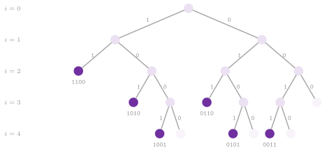
Figure 19.1 shows the tree of the calls for \(n = 4\) and \(k = 2\); the solutions come in the decreasing order of their vectors read as binary numbers, since the place in is tried first. Note that the text of the book counts the subsets as \(n! / ( n - k )!\), which is the number of their orderings; the subsets of \(k\) items are \(\binom{n}{k} = n! / ( k! ( n - k )! )\), as the header states.
Lemma 19.2. For \(k \le n\), subsets( n , k , f ) visits
at most \(( n + 1 ) \binom{n}{k}\) nodes that are not pruned, and at most as
many pruned ones; hence it costs \(O( n \binom{n}{k} )\) time, i.e., \(O( n )\)
per subset, and \(O( n )\) space.
Proof. A node \(( i , c )\) (the place \(i\), with \(c\) items in) that is not pruned has \(c < k\) and \(c + ( n - i ) \ge k\), and hence at least one solution below it (put in the next \(k - c\) places). It therefore lies on one of the \(\binom{n}{k}\) paths from the root to a solution, each of at most \(n + 1\) nodes. Its child "in" is never pruned, since \(i + 1 = n\) would give \(c + 1 = k\), a solution; its child "out" is pruned only if \(c + ( n - i ) = k\). Each pruned node is thus the child of a distinct node that is not pruned. \(\square\)
permutations( A , f ) visits the \(n!\) permutations of the items of \(A\),
each place taking in turn every item not used yet; the items are told
apart by their places, and equal items give each permutation of the values
more than once. derangements( A , f ) prunes the item of the place \(i\) at
the place \(i\), and visits the permutations in which no item is in its own
place (again by places, not by values).
Lemma 19.3. The tree of permutations()
has
nodes; hence the enumeration costs \(O( n \cdot n! )\) time, i.e., \(O( n )\) per permutation.
Proof. A node of the depth \(i\) is an ordered choice of \(i\) distinct places among \(n\), and there are \(n! / ( n - i )!\) of them; the sum is rewritten with \(j = n - i\), and it is bounded by the series of \(e\). Each node scans the \(n\) flags \(\mathit{used}\), which costs \(O( n )\). \(\square\)
Pruning only removes nodes, and hence the tree of derangements() has
fewer than \(e \, n!\) nodes too, while the derangements of \(n\) items are
\(D_n = \lfloor n! / e + 1 / 2 \rfloor\), i.e., \(n! \le e ( D_n + 1 / 2 )\).
For \(n \ge 2\), where \(D_n \ge 1\), the nodes are therefore fewer than
\(e^2 ( D_n + 1 / 2 ) \le 1.5 \, e^2 D_n\), and the enumeration costs
\(O( n )\) time per derangement as well (some of these nodes are dead ends,
e.g., a last place left with its own item only).
Finally, subsetSum( A , k , f ) visits the subsets of the positive items
of \(A\) whose sum is \(k\), as the lists of their places. Its pruning rests on
the positivity of the items: a partial sum larger than \(k\) cannot come
back, since no item added later can lower it, and the branch is cut as
soon as \(s + A[ j ] > k\).
All the functions of the area are written on the same pattern (a
recursive lambda over the state, a counter of the solutions, and a flag
that stops the visit as soon as f returns true), and they are called as
in the following lines, which print the six subsets of
Figure 19.1 in the order of the figure and
return 6:
#include "ADS/backtrack/Enumeration.h"

long c = ADS::subsets( 4 , 2 , []( const std::vector< bool > & S ) {
 for( bool b : S )
  std::cout << b;  // 1100 , 1010 , ... , 0011
 std::cout << '\n';
 return( false );  // go on: all the subsets
 } );
19.3 The \(n\) queens¶
In the problem of the \(n\) queens one looks for the placements of \(n\) queens on an
\(n \times n\) board, no two on a row, a column or a diagonal (exercise 16.5
of Montresor 2025). Since two queens
on a row attack each other, each row holds one queen, and a solution is
the vector \(Q\) of their columns, \(Q[ r ]\) the column of the queen of the
row \(r\). Such a vector is a permutation; hence the candidates are \(n!\)
instead of the \(\binom{n^2}{n}\) placements of \(n\) queens on the board. Two queens
\(( r , Q[ r ] )\) and \(( r' , Q[ r' ] )\) share a diagonal if and only if
\(| Q[ r ] - Q[ r' ] | = | r - r' |\), which is the test of admissible(),
\(O( n^2 )\) on a whole placement, and of the iterative version
nQueensIterative(), \(O( r )\) for the queen of the row \(r\).
In nQueens(), instead, the test of a choice costs \(O( 1 )\), since the
function keeps three sets of the columns attacked on the current row \(r\): \(C\), the
columns taken; \(D_1\), the columns attacked along the diagonals that go down
to the right; and \(D_2\), those attacked along the diagonals that go down to
the left
(Algorithm 19.2). Moving to the next row shifts
\(D_1\) by one column to the right and \(D_2\) by one to the left, and the free
columns of a row are the complement of \(C \cup D_1 \cup D_2\).
Algorithm 19.2. The \(n\) queens with the attacked columns as sets (Montresor 2025, exercise 16.5).
Lemma 19.4. At the row \(r\), the set \(D_1\) of Algorithm 19.2 is the set of the columns \(Q[ r' ] + ( r - r' ) < n\) for \(r' < r\), and \(D_2\) that of the columns \(Q[ r' ] - ( r - r' ) \ge 0\); hence a column \(c\) is free on the row \(r\) if and only if the queen \(( r , c )\) attacks none of the queens above it.
Proof. By induction on \(r\); both sets are empty at the row 0. Line 5 adds the column \(c = Q[ r ]\), at the distance 0 from its row, and adds 1 to (resp. subtracts 1 from) each column of the set, dropping those that leave the board; this keeps the invariant at the row \(r + 1\). Finally, the queen \(( r , c )\) attacks the queen \(( r' , Q[ r' ] )\) along a diagonal if and only if \(c = Q[ r' ] \pm ( r - r' )\). \(\square\)
As masks of \(n \le 32\) bits, the three sets cost a few operations on a word: the shift of \(D_1\) is a shift left by one place with the mask of the \(n\) places, that of \(D_2\) a shift right, and the free columns are visited from the lowest 1 of \(\lnot ( C \mid D_1 \mid D_2 )\), by the identities of §18.2 (cf. (18.1)). Each node of the tree thus costs \(O( 1 )\), and the tree has at most \(e \, n!\) nodes by (19.1). Table 19.1 follows the masks along the path to the first solution for \(n = 4\).
Table 19.1. nQueens( 4 , f ) along the
path to its first solution \(Q = ( 1 , 3 , 0 , 2 )\): the sets of the columns
at each row, the free ones and the column chosen (the least free one that
leads to a solution; at the row 0 the column 0 is tried first and fails).
| Row \(r\) | \(C\) | \(D_1\) | \(D_2\) | Free | \(Q[ r ]\) |
|---|---|---|---|---|---|
| 0 | \(\emptyset\) | \(\emptyset\) | \(\emptyset\) | \(\{ 0 , 1 , 2 , 3 \}\) | 1 |
| 1 | \(\{ 1 \}\) | \(\{ 2 \}\) | \(\{ 0 \}\) | \(\{ 3 \}\) | 3 |
| 2 | \(\{ 1 , 3 \}\) | \(\{ 3 \}\) | \(\{ 2 \}\) | \(\{ 0 \}\) | 0 |
| 3 | \(\{ 0 , 1 , 3 \}\) | \(\{ 1 \}\) | \(\{ 1 \}\) | \(\{ 2 \}\) | 2 |
For \(n = 1 , \ldots , 10\) the solutions are \(1 , 0 , 0 , 2 ,
10 , 4 , 40 , 92 , 352 , 724\), and the tests check them. Note that the
masks need \(n \le 32\), which the contract checks; at the contract level 3
each solution is also checked by admissible(). Finally, board( Q )
draws a placement as a string of \(n\) lines, one per row, with the letter Q
for a queen and a dot for an empty square. Many more results
on the problem, including the placements that can be written down directly
without search, are in the survey of Bell and Stevens
2009.
19.4 The tour of the knight, the Sudoku and the anagrams¶
The tour of the knight. knightTour( n , x , y , warnsdorff ) looks
for a path of the knight that visits each square of an \(n \times n\) board
once, from the square \(( x , y )\) (exercise 16.6 of Montresor
2025). This is a Hamiltonian path
from \(( x , y )\) in the graph of the moves of the knight, whose nodes are
the \(n^2\) squares and have degree at most 8. Our backtrack extends the path
by a move to a square not visited yet, and goes back from a square with no
such move. It returns the board with the step of each square, from 1, or
no board if there is no tour from \(( x , y )\).
Algorithm 19.3. The tour of the knight, in the order of the book or by the rule of Warnsdorff.
In the order of the book (the 8 moves always in the same order) the tree may be explored for a long time before a tour is found. Instead, the rule of Warnsdorff 1823 tries first the moves to the squares with the fewest onward moves (line 7, a stable sort, so that ties keep the order of the book), i.e., it visits first the squares that would otherwise become dead ends. It is a heuristic, with no bound on the backtracks that it saves; yet, on the boards of practical size it usually finds a tour almost without going back. On the \(5 \times 5\) board from a corner, e.g., the order of the book makes 329 calls of \(\mathrm{tour}()\) before it finds the tour of Table 19.2 (left), while the rule of Warnsdorff makes 25, one per square, and 64 on the \(8 \times 8\) board.
Table 19.2. The tours of the knight of
knightTour( 5 , 0 , 0 ) on the \(5 \times 5\) board, the step of each
square, in the order of the book (left) and by the rule of Warnsdorff
(right).
| Book | Warnsdorff | |||||||||
|---|---|---|---|---|---|---|---|---|---|---|
| 1 | 14 | 9 | 20 | 23 | 1 | 24 | 13 | 18 | 7 | |
| 10 | 19 | 22 | 15 | 8 | 14 | 19 | 8 | 25 | 12 | |
| 5 | 2 | 13 | 24 | 21 | 9 | 2 | 23 | 6 | 17 | |
| 18 | 11 | 4 | 7 | 16 | 20 | 15 | 4 | 11 | 22 | |
| 3 | 6 | 17 | 12 | 25 | 3 | 10 | 21 | 16 | 5 |
A tour need not exist: there is none on the boards of side 2, 3 and 4.
On the \(5 \times 5\) board there is none from a square of the color other
than that of the corners, since the knight changes color at each move and
that color has 12 squares against 13. In these cases the backtrack proves
the absence by exhausting the tree, and the test ch16.ex16.6 checks these
cases with both orders of the moves.
The Sudoku. sudoku( S ) fills the empty squares (the zeros) of a
Grid, i.e., a vector of rows of int, of side \(N = n^2\) in the order of the rows, each with a number of
\(1 , \ldots , N\) that is not on its row, its column or its block of
\(n \times n\) squares (check(), \(O( N )\)), and skips the squares given
(section 16.3 and exercise 16.7 of Montresor
2025); it returns true, with the grid
filled, if it can.
Its tree has depth \(n^4\) and at most \(N\) children per node. For the classic
\(n = 3\) the cost is therefore bounded by a constant (a "huge" one), and it
presumably grows superpolynomially with \(n\), since the completion of a
Sudoku of side \(n^2\) is known to be NP-complete. In practice the
order of the rows is a poor one: the exact cover of
§19.5 chooses at each step the square (or the
row, column or block) with the fewest candidates, which typically shrinks
the tree by orders of magnitude, and the test taocp.dancing-links solves
the same grid both ways.
The anagrams. anagrams( s , word , prefix ) returns the strings made
of all the characters of \(s\), in any order, that split into words for which
word( w ) is true, written with one blank between the words (exercise
16.8 of Montresor 2025). Its
backtrack chooses the characters one at a time, as the permutations do,
but takes each distinct character once per place, from the multiset \(L\)
of the characters left. Hence each permutation of the multiset is built
once, and no anagram comes twice. After each character, the word being
built either goes on or, if it is a word, ends there. Also, the test
prefix( w ), true when \(w\) begins some word, prunes a branch as soon as
its current word cannot be completed; on a real dictionary it typically
removes most of the \(n! / \prod_c m_c!\) permutations (\(m_c\) the
multiplicity of the character \(c\)).
19.5 Exact cover and the dancing links¶
We now leave the exercises of the book. Let a set of items be given, some primary and some secondary, together with a family of options, each a set of items. An exact cover is a set of options that contains each primary item once and each secondary item at most once (Knuth 2022, §7.2.2.1). Many puzzles are exact covers. For instance, the \(n\) queens have the rows and the columns as primary items and the \(2 ( 2 n - 1 )\) diagonals as secondary ones, with an option per square (its row, its column and its two diagonals); the Sudoku has 324 primary items (a square, a row with a number, a column with a number, a block with a number) and an option for each number that a square may take. Knuth's search, his Algorithm X, is a backtrack whose place is a primary item not covered yet, and whose choices are the options that contain it and none of the items already covered; choosing an option covers its items and removes from the problem each option that meets one of them.
ExactCover of DancingLinks.h realizes Algorithm X on the dancing
links of Knuth 2000. There the primary
items are a circular doubly linked list (the links \(L\) and \(R\), with the head 0),
and each secondary item is a list with no other item. An option is a set
of nodes, one per item, each in the vertical circular list of the nodes of
its item (the links \(U\) and \(D\), with the head of the item, whose
\(\mathit{len}\) counts the nodes). Furthermore, the nodes of an option are consecutive
in the arrays, which lets the code walk an option by the index, and
addOption( items ) appends one at the bottom of the list of each of its
items and returns its index. All the method
rests on the following property of the doubly
linked lists (Figure 19.2).
Lemma 19.5. On a circular doubly linked list, the removal of a node \(x\) by
leaves \(L[ x ]\) and \(R[ x ]\) as they were; hence the assignments \(R[ L[ x ] ] \gets x\) and \(L[ R[ x ] ] \gets x\) put it back, provided that the removals made after that of \(x\) have been undone before, in the reverse order.
Proof. Since the assignments (19.2) write only the links of the neighbors of \(x\), they leave \(L[ x ]\) and \(R[ x ]\) unchanged. Once the later removals are undone, in the reverse order, the list is the one right after the removal of \(x\) (by induction on their number), in which the node after \(L[ x ]\) is \(R[ x ]\); hence the two assignments make \(x\) again the neighbor of both. \(\square\)
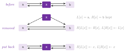
Covering an item \(i\) takes it off the list of the items and hides each option that contains it, i.e., takes the other nodes of the option off their vertical lists (and decrements the \(\mathit{len}\) of their items); uncovering undoes the same steps in the reverse order (Algorithm 19.4).
Algorithm 19.4. Algorithm X on the dancing links (Knuth 2022, §7.2.2.1; Knuth 2000).
The interface of the class is made of four members: the items are numbered
from 0, the first primary of them primary and the next secondary ones
secondary, and solve() calls visit( options ) on each solution, with
the indices of its options in the order in which they were chosen, until
visit returns true; it returns the number of the solutions visited.
// declarations of <ADS/backtrack/DancingLinks.h>
ExactCover( int primary , int secondary = 0 );
int addOption( const std::vector< int > & items );  // its index
template< class F >
long solve( F && visit );
long updates( void ) const;  // the links updated
For instance, on the three primary items \(0 , 1 , 2\) and the options \(\{ 0 , 1 \}\), \(\{ 2 \}\), \(\{ 1 , 2 \}\) and \(\{ 0 \}\) (with the indices 0 to 3), the search branches on the item 0, which has two options, and visits the two exact covers \(( 0 , 1 )\) and \(( 3 , 2 )\):
ADS::ExactCover X( 3 );
for( auto o :
     std::vector< std::vector< int > >{ { 0 , 1 } , { 2 } , { 1 , 2 } ,
                                        { 0 } } )
 X.addOption( o );
long s = X.solve( []( const std::vector< int > & o ) {
 return( false );  // ( 0 , 1 ) , then ( 3 , 2 )
 } );                // s == 2
Lemma 19.6. ExactCover::solve() visits
each exact cover once, and the links after the search are those before
it.
Proof. At a node of the search, the items on the list are the primary
items not covered yet, and the options on the vertical lists are those that
meet no covered item; this holds at the root and is kept by cover().
Hence the choices at the item \(i\) are the options that may still cover it, and a solution is reached when the list of the primary items is
empty. Furthermore, an exact cover contains one option with the item \(i\)
chosen at a node, and hence it lies below one child only of each node on
its path; by Lemma 19.1 it is
visited once. Finally, the calls of uncover() mirror those of
cover() in the reverse order, and by
Lemma 19.5 they restore the links; the class
checks this as an audit. \(\square\)
Each removal and each reinsertion costs \(O( 1 )\), and the work of a node
of the tree is the number of links updated, the measure of Knuth that
updates() returns. At each level the search branches on the primary item with the
fewest options left (the "minimum remaining values" heuristic, MRV): an
item with none ends the branch at once, and an item with one forces its
option without branching, which usually keeps the tree small. Note that an
option made of secondary items only is refused by the contract, since it
would never be chosen. Our test taocp.dancing-links counts the \(n\) queens as
exact covers against nQueens(), solves the Sudoku of sudoku(), and
compares random small instances with the enumeration of all the subsets of
options.
19.6 Exact cover with colors on sparse sets¶
FastExactCover solves the exact cover with colors, Knuth's Algorithm C,
in which an option may give a color to a secondary item, and several
options may share the item if they give it the same color (an uncolored
secondary item is still taken at most once). Without colors it is the
exact cover of §19.5, with the same solutions
visited in another order (possibly); its addOption( items , colors )
takes the color of each item, 0 (or no colors) for none. Its engineering
replaces the linked lists by
sparse sets (Briggs and Torczon 1993),
the "dancing cells" of Knuth's program SSXCC (Knuth
2023). All the nodes of the options
are one array of records \(\{ \mathit{item} , \mathit{loc} , \mathit{color} \}\)
of 16 bytes (with one int of padding); those of an option are consecutive and followed by a
spacer whose item is minus the size of the option, and hence the other
nodes of an option are walked by the index. Each item \(x\) has a segment of
an array \(\mathit{set}\), whose first \(\mathrm{size}( x )\) entries are its
active options, and each node knows its place \(\mathit{loc}\) in the
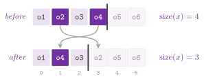
segment of its item. An option leaves the set of \(x\) by a swap with the last active
entry and a decrement of \(\mathrm{size}( x )\), in \(O( 1 )\)
(Figure 19.3), and the active items form a
sparse set too, with the place \(\mathrm{pos}( x )\) of each.
Lemma 19.7. Let the sizes of the active items be saved at a level of the search. After any sequence of removals by swaps from the sets of those items, writing the saved sizes back makes the active entries of each set the same as at the save, possibly in another order.
Proof. A removal swaps two entries among the first \(\mathrm{size}( x )\) of the segment of \(x\), and then decrements \(\mathrm{size}( x )\); it never moves an entry out of the first \(s\) places, for the size \(s\) at the save, since the sizes only decrease after it. Hence the first \(s\) entries are, at any later time, a permutation of the entries that were active at the save; the entries removed are among them, after the active ones. \(\square\)
Restoring a level therefore needs no inverse swap, only the sizes written back. This costs \(O( a )\) per level for \(a\) active items, against an update per link of the dancing links; also, the memory is read by consecutive indices rather than by pointers. At each level the search (Algorithm 19.5) takes the active primary item \(x\) of least \(\mathrm{size}( x )\) (ties to the least index), takes it out of the active items, hides its options from the other items, and pushes the sizes of the active items on a stack. Then each option of \(x\) in turn takes its other items out and hides their incompatible options (all of them for a primary or uncolored item, those of another color for a colored one), and the search goes one level deeper.
Algorithm 19.5. Algorithm C on sparse sets
(Knuth 2022, §7.2.2.1; Knuth
2023); the code keeps the levels on
a stack of its own, with goto between the steps as in the program of
Knuth.
Hiding an option checks the size of each primary item that it leaves: a size 0 abandons the choice at once, before going deeper, and a size 1 makes the item a forced move, taken at the next level without saving the sizes (its only option needs no return). This check is made in the loop that updates the sets (lines 17 and 18 of Algorithm 19.5), which therefore serves both purposes. Note that the hiding of line 6 is made without it: an item \(u\) whose options all contain \(x\) drops to the size 0 there, and yet it is no dead end, since the option of \(x\) chosen at line 8 covers it too.
Lemma 19.8. FastExactCover::solve()
visits each exact cover with colors once, as the list of its options.
Proof. We show that, at the entry of a level, (i) the active items are the primary items not covered by the options chosen and the secondary items that they do not contain, and (ii) the first \(\mathrm{size}( u )\) entries of \(\mathit{set}( u )\), for an active item \(u\), are the options that contain \(u\) and are compatible with the options chosen, i.e., that contain no primary or uncolored item covered by them and give each colored item met by them its color. Both hold at the root, where nothing is chosen. When the option \(o\) of \(x\) is chosen, lines 6 and 9 take \(x\) and the other items of \(o\) out of the active ones, and lines 6 and 10 remove from the sets of the items left active exactly the options that \(o\) makes incompatible: those with \(x\) or with a primary or uncolored item of \(o\) (all of the options of such an item), and those that give a colored item of \(o\) another color. Hence (i) and (ii) hold one level deeper, and by Lemma 19.7 they hold again at each option tried after the sizes are written back at line 12. By (i) a solution is visited when no primary item is active, and by (ii) the options chosen are then compatible, i.e., an exact cover with colors. The branches cut are those of lines 5 and 17, where an active primary item has no compatible option left, and which therefore hold no solution; and a forced item (line 2) is a branch with one choice, for which the sizes saved by the level above suffice, since it changes only the sizes of items active there. Finally, a solution has exactly one option with the item \(x\) chosen at a level, so that it lies below one child of each node of its path, and Lemma 19.1 gives the claim. \(\square\)
The interface is that of ExactCover, with the colors of the items of an
option (0, or no colors, for none) and the count of the nodes of the
tree:
// declarations of <ADS/backtrack/FastExactCover.h>
FastExactCover( int primary , int secondary = 0 );
int addOption( const std::vector< int > & items ,
               const std::vector< int > & colors = {} );
template< class F >
long solve( F && visit );
long updates( void ) const;  // the options moved
long nodes( void ) const;    // the nodes visited
The time is \(O( 1 )\) per update of a set, and updates() and nodes()
count the updates and the nodes of the tree. In both classes the worst
case stays exponential, the exact cover being NP-complete; the comparison
of the two on the same instances, and with the program of Knuth, belongs to
the campaign of Appendix B. Finally, the test
engineered_combinatorial.fast-exact-cover checks that FastExactCover
finds the same solutions as ExactCover on random instances, and the
colors against an enumeration.
19.7 Satisfiability¶
A formula in conjunctive normal form is a set of clauses, each a
disjunction of literals, i.e., of variables and of negated variables; it
is satisfiable if some assignment of truth values makes each clause true
(a model). In the library a literal is the integer \(v + 1\) or
\(-( v + 1 )\) for the variable \(v \in [ 0 , n )\), and the type Cnf with
the checker satCertificate() comes from ADS/complexity/Problems.h
(cf. Chapter 20). Under a partial assignment, a clause is satisfied if one
of its literals is true, conflicting if all are false, and unit if all
are false but one, which is free and then must be true in each model that
extends the assignment.
Lemma 19.9. Making true the free literal of a unit clause, until no clause is unit or one is conflicting, loses no model of the formula that extends the assignment; a conflicting clause proves that there is none.
Proof. A model that extends the assignment makes the unit clause true, and its other literals are false; hence it makes the free literal true, and it extends the new assignment too. A conflicting clause is false under any extension. \(\square\)
DPLL. In the procedure of Davis, Putnam, Logemann and Loveland (Davis and
Putnam 1960; Davis et al.
1962) this propagation alternates with a
branch on a free literal, both values tried, and the search goes back on a
conflict
(Algorithm 19.6). dpll( F , n ) branches on
the first free literal of a shortest open clause, which makes the
propagation of the branch likely to produce more units. It returns a model
(the variables left free set to false), or no model if there is none.
Algorithm 19.6. DPLL (Davis et al. 1962).
By Lemma 19.1 and
Lemma 19.9 the procedure is complete, and its
tree has at most \(2^n\) leaves for \(n\) variables. It is fair to remark,
however, that the propagation of dpll() scans all the clauses at each
pass, and possibly \(n\) passes per node; the procedure is thus simple and
slow, and it serves as a reference.
Conflict-driven clause learning. BasicCdcl is the method of the
modern solvers (Marques-Silva and Sakallah
1999; Moskewicz et al.
2001; Knuth 2022,
§7.2.2.2). It keeps the literals assigned
in a trail, each with its level (the number of decisions before it) and
its reason (the clause that forced it, none for a decision); a variable
is decided only when the propagation has no literal left to force
(Algorithm 19.7).
Algorithm 19.7. Conflict-driven clause learning, with the propagation on two watched literals and the analysis to the first unique implication point.
Watched literals. Each clause of at least two literals watches two of them, the first two of its vector (a unit clause is an assignment of the level 0). When a literal becomes false, the propagation visits only the clauses that watch it. If the other watched literal is true, the clause is satisfied; otherwise the propagation looks for another literal that is not false and watches it instead, and if there is none the clause is unit (the other watch is forced) or conflicting. This is \(\mathrm{propagate}()\), lines 15 to 22 of Algorithm 19.7, where a watch moved is swapped into the second place of the vector. Its invariant, and the reason why going back needs no update of the watches, are as follows; we call pending a literal of the trail that \(\mathrm{propagate}()\) has not visited yet.
Lemma 19.10. At each call of \(\mathrm{propagate}()\), for each clause \(c\) of at least two literals and each watched literal \(w\) of \(c\) that is false, either \(\lnot w\) is pending, or the other watched literal \(w'\) of \(c\) is true and its level is at most that of \(w\). Hence, when \(\mathrm{propagate}()\) returns no conflict, no clause is unit or conflicting.
Proof. At the first call only the unit clauses of the formula are assigned, all of them pending. Within a call, the pending literals are of the current level: after the constructor only the level 0 exists, and a jump back or a restart sets the head of the trail to its end before the first literal of the new level is assigned. When the pending \(\lnot w\) is visited, \(\mathrm{propagate}()\) looks at each clause \(c\) that watches \(w\). If \(w'\) is true, its level is at most the current one, which is that of \(w\). If a literal not watched is not false, it replaces \(w\), and \(c\) has a false watch only if \(w'\) is false, in which case \(\lnot w'\) is pending (otherwise, by the invariant when it was visited, \(w\) would have been true). Otherwise \(w'\) is either false, a conflict, or free, and then it is assigned at the current level with the reason \(c\), which satisfies the condition with equal levels. Cancelling the levels above \(b\) removes \(w'\) only if its level exceeds \(b\), and then also the false \(w\), of a level at least as large; the pending literals skipped at a conflict are all of the current level, which the jump back cancels. A learned clause watches \(\lnot p\), assigned at the level \(b\) of the jump, and a literal of the level \(b\) (the code moves one of the largest level of \(C\) to the second place). Finally, if no conflict is returned, nothing is pending, and each clause with a false watch has a true one, i.e., it is satisfied; the others have two literals that are not false, and are neither unit nor conflicting. \(\square\)
The analysis of a conflict. One resolves the conflicting clause with the reasons of its literals of the current level, from the last one assigned backwards, until a single literal of that level is left, the first unique implication point \(p\) (lines 23 to 31 of Algorithm 19.7). What is learned is the clause of \(\lnot p\) together with the literals of the lower levels met on the way; the search then jumps back to the largest of their levels, where the clause forces \(\lnot p\).
Lemma 19.11. The learned clause \(C\) is
implied by the formula, it is false under the trail at the conflict, and
after the levels above the second largest level of its literals are
cancelled it is unit, with \(\lnot p\) free; hence it forces \(\lnot p\) there,
and the assignment of the conflict cannot occur again. The search is
complete, and solve() ends with SAT or UNSAT when no bound of conflicts is
given. (With a bound maxConflicts, the third value of the enumeration
Result, UNKNOWN, is returned when the conflicts allowed are over.)
Proof. Resolution preserves the models, and each step resolves the clause at hand with a clause of the formula or a learned one, which are implied by induction. At each step the clause is false, since its literals are false under the trail. At the end it has one literal of the current level, \(\lnot p\), while the others have smaller levels, the largest of which is \(b\); after the levels above \(b\) are cancelled they are still false while \(p\) is free, and the clause is unit. Moreover, \(C\) was not among the clauses of the solver before the conflict: it would have been unit at the level \(b\), and since a decision is taken only when the propagation has no literal left to force (Lemma 19.10), \(\lnot p\) would have been assigned at that level, before the decision of the current one. Hence each conflict adds a new clause (a learned unit clause is kept as an assignment of the level 0, which neither a jump back nor a restart cancels), the clauses on \(n\) variables are at most \(3^n\), and the number of conflicts is finite; the restarts do not change this, since they keep the learned clauses. Between two conflicts at most \(n\) decisions are taken, and hence the search ends. It answers SAT only when every variable is assigned with no conflict, i.e., on a model; and it answers UNSAT only on a conflict at the level 0, where every literal of the trail is forced by the formula and by clauses implied by it, so that by Lemma 19.9 no model exists. \(\square\)
Decisions and restarts. Each decision takes the free variable of largest
activity, which grows at each conflict for the variables met in
the analysis, and decays by the increase of the increment (the factor
\(1 / 0.95\) at each conflict, the VSIDS rule of Moskewicz et al.
2001). A variable chosen takes the value
that it had last (the phase saving of Pipatsrisawat and Darwiche
2007). We keep the variables in
a lazy heap: a raised activity pushes a new pair \(( \mathit{activity} , v )\),
the stale ones are dropped when they reach the top, and the activities are
rescaled by \(10^{-100}\) when one of them exceeds \(10^{100}\). A restart
cancels all the levels after \(100 \, \mathrm{luby}( k )\) conflicts for the
\(k\)-th restart, and keep the learned clauses and the activities. Here
\(\mathrm{luby}\) is the sequence \(1 , 1 , 2 , 1 , 1 , 2 , 4 , \ldots\) of
Luby et al. 1993, which for a search of
unknown length is within a logarithmic factor of the best strategy of
restarts (in their model of Las Vegas algorithms, at least). Learned
clauses are never deleted, which suits formulae of moderate size; also, an
unsatisfiable formula comes with no certificate (a proof of the learned
clauses, as in the format DRAT, would be one). Note that the heap is a parameter of the class:
Cdcl is BasicCdcl on std::priority_queue, and the heaps of Boost and
the DaryHeap of Chapter 9 give the same decisions
and conflicts, since the pairs are ordered totally.
19.8 Discussion and references¶
The backtrack of §19.1 to
§19.4 follows chapter 16 of Montresor
2025, with its exercises; the rule of
the knight goes back to Warnsdorff 1823,
and Bell and Stevens 2009 survey the \(n\)
queens. Both the exact cover and the dancing links are those of Knuth
2000 and of Knuth 2022,
§7.2.2.1, where Algorithm C adds the
colors; the sparse sets are due to Briggs and Torczon
1993, and their use in the exact cover
to the program SSXCC of Knuth 2023.
DPLL is the procedure of Davis and Putnam
1960 with the branching of Davis et al.
1962, and the learning of clauses is that of
GRASP (Marques-Silva and Sakallah
1999), with the watched literals
and the activities of Chaff (Moskewicz et al.
2001), and Knuth 2022,
§7.2.2.2 describes all of them. Our
solvers are meant to be read, and to be compared on the
same decisions; the industrial solvers add the deletion of the learned
clauses, the preprocessing and many other refinements, and we make no
claim of competing with them. Comparing the two exact covers, and
of the heaps under BasicCdcl, is left to the campaign of Appendix B.
19.9 Exercises¶
Each exercise names the test of the library that solves it (run it with
ctest -R <name>).
- Enumerate the subsets of \(k\) of \(n\) items by backtrack, pruning the
nodes with \(k\) items in or with too few items left, and count them
against \(\binom{n}{k}\). Test:
ch16.sec16.2.subsets. - Enumerate the permutations of \(n\) items, and their derangements, by
backtrack, and check the numbers \(n!\) and \(!n\). Tests:
ch16.ex16.2,ch16.ex16.3. - Enumerate the subsets of positive items whose sum is \(k\), pruning a
branch as soon as its sum exceeds \(k\). Test:
ch16.ex16.4. - Count the placements of \(n\) queens with the attacked columns and
diagonals kept as masks of bits, and check the counts for
\(n = 1 , \ldots , 10\). Test:
ch16.ex16.5. - Write the backtrack of the \(n\) queens without recursion, keeping the
place \(k\) and the vector \(V\) of the choices. Test:
beyond.nqueens-iterative. - Find a tour of the knight by the plain backtrack and by the rule of
Warnsdorff, and show that there is none on the boards of side 3 and 4
and from a square of the wrong color on the \(5 \times 5\) board. Test:
ch16.ex16.6. - Solve a Sudoku by backtrack, with
check()testing the row, the column and the block of a square. Tests:ch16.sec16.3.sudoku,ch16.ex16.7. - Find the anagrams of a string that split into the words of a
dictionary, each one once, pruning by the prefixes of the words. Test:
ch16.ex16.8. - Solve the exact cover on dancing links, count the \(n\) queens as exact
covers, and solve the Sudoku as one. Test:
taocp.dancing-links. - Solve the exact cover with colors on sparse sets, and check that it
finds the same solutions as the dancing links. Test:
engineered_combinatorial.fast-exact-cover. - Decide the satisfiability of random 3-SAT formulae at the threshold by
DPLL and by clause learning, and prove the pigeonholes unsatisfiable.
Test:
taocp.sat-solvers. - Enumerate the derangements of \(n\) items, and check them against the
permutations of
std::next_permutationwith no fixed point and their number against the recurrence \(D_n = ( n - 1 ) ( D_{n-1} + D_{n-2} )\). Test:exam_backtrackb.backtrack-47.