12. Sorting¶
[Source: include/ADS/sort/Sort.h, Sorted.h, SelectionSort.h,
InsertionSort.h, ExchangeSorts.h, ShellSort.h, KnuthSorts.h,
MergeSort.h, RunSorts.h, StrandSort.h, TreeSort.h, QuickSort.h,
QuicksortAdversary.h, EngineeredQuickSorts.h, PdqSort.h,
VectorQuickSort.h, SampleSort.h, LearnedSort.h, Heapsort.h,
CountingSort.h, PigeonholeSort.h, RadixSort.h, MultikeyQuickSort.h,
StringSort.h, SortingNetworks.h, ExternalSort.h]
We are concerned in this chapter with the rearrangement of a vector \(A[ 0 .. n - 1 ]\) into non-decreasing order, i.e., so that
where \(\le\) is a total preorder given by the comparator less of the call
(the relation \(a < b\) being less( a , b )). In ADS/sort the headers
realize the sorts of Montresor 2025
(the elementary ones of its section 2.7, Quicksort of section 12.2, heapsort
of section 10.1.4 and Shell Sort of section 15.1) and those of chapter 11 of
Morin 2013, with their exercises. Many more
go beyond both books: the internal sorts of Knuth
1998 that the textbooks leave out, the
sorts engineered for the caches and for the vector registers of today,
samplesort and the learned sort, the sorts of strings, the sorting networks
and the sort of a file larger than the memory. Of all of them, sort() and
stableSort() of Sort.h choose one for each input
(§12.14). We open the chapter with the definitions
(§12.1) and with the lower bound that no sort by
comparisons can beat (§12.2). It then follows the
families of algorithms, from the elementary sorts to the sorts by digits,
giving for each one the property on which its correctness rests and the
argument behind its bound. In the sets of
§1.9, LearnedSort.h, PdqSort.h (the
quicksort of Peters, which EngineeredQuickSorts.h includes),
QuicksortAdversary.h, RadixSort.h, RunSorts.h, SampleSort.h,
Sort.h, StringSort.h and VectorQuickSort.h are advanced and the other
headers of this chapter are base, while Sorted.h is in the core that the
two sets include.
12.1 Definitions and notation¶
Two items are equal when neither is smaller than the other, which need not
make them the same item (e.g., two records with the same key). A sort
is stable (Montresor 2025, §12.5)
if the equal items keep the order that they had in the input, which matters,
e.g., when records are sorted by one of their fields, and it is in
place if it uses \(O( 1 )\) extra items, or \(O( \log n )\) extra words for a
stack. A sort by comparisons learns about the items only through less,
and works therefore with any order. The sorts by digits (counting,
pigeonhole and radix sorts) read the keys as integers or strings instead,
and are not bound by the lower bound of §12.2.
Unless stated otherwise, a sort of the library sorts a
std::vector in place, with the comparator as its last parameter but the
optional counters, e.g.,
// declarations of <ADS/sort/Sort.h>
template< class T , class C = std::less<> >
void sort( std::vector< T > & A , C less = C() );
template< class T , class C = std::less<> >
void stableSort( std::vector< T > & A , C less = C() );
template< SortStore Store ,
          class T =
            std::ranges::range_value_t< std::remove_cvref_t< Store > > ,
          class C = std::less<> >
void sort( Store && A , C less = C() );
template< SortRange R , class... P >
 requires requires( std::vector< std::ranges::range_value_t< R > > & v ,
                    P &&... p )
{ sort( v , std::forward< P >( p )... ); }
decltype( auto ) sort( R && A , P &&... p ) { ... }
so that ADS::sort( A ) sorts \(A\) in increasing order and
ADS::sort( A , std::greater<>() ) in decreasing order. Every sort that
takes a whole vector is a template on the storage of the items, taken by
reference (the concept SortStore, i.e., a std::vector or a
std::span), and the overload on a vector is one call of it, inlined, so
that a vector is sorted by the same code as before; it takes as well, as
in the last declaration, a SortRange of ADS/sort/Sorted.h, i.e., any
other sized random-access range of movable items (an array, a
std::deque, a TieredVector, the vectors of Boost or Eigen), with the
other arguments as for the vector. A contiguous range is sorted in place as
the span of its items. On a range that is not contiguous, the sorts of the
book, which read the items only by their ranks, also work in place (on the
view of the range, the concept RankStore), while the engineered sorts,
whose code reads the items by their addresses, move them into a vector,
sort them there and move them back (\(2 n\) moves and \(n\) items of memory),
as the comment of each says; the parallel sorts of
§25.7 do the same after their executor.
Table 12.1 fixes the symbols that the rest of the chapter uses.
Table 12.1. The symbols of the chapter.
| Symbol | Meaning |
|---|---|
| \(n\), \(A[ 0 .. n - 1 ]\) | the number of items and the vector that holds them, \(A[ \mathit{lo} .. \mathit{hi} - 1 ]\) a part of it |
| \(I( A )\) | the inversions of \(A\), the pairs \(i < j\) with \(A[ j ] < A[ i ]\) (countInversions()) |
| \(r\), \(\ell_1 , \ldots , \ell_r\) | the runs of \(A\), its maximal non-decreasing (or strictly decreasing) stretches, and their lengths |
| \(H\) | the entropy \(\sum_i ( \ell_i / n ) \log_2 ( n / \ell_i )\) of the lengths of the runs |
| \(k\) | the number of distinct keys, or the range \([ 0 , k )\) of integer keys |
| \(w\) | the bytes (or bits) of a key read by a radix sort |
| \(D\) | the total length of the distinguishing prefixes of a set of strings |
| \(\sigma\) | the size of the alphabet of the strings, 256 for the bytes |
| \(W\) | the lanes of a vector register, 4 to 16 keys |
| \(H_n\) | the harmonic number \(\sum_{i=1}^{n} 1 / i = \ln n + O( 1 )\) |
We remark that \(0 \le I( A ) \le n ( n - 1 ) / 2\), the two ends attained by a sorted and by a reversed vector of distinct items, and that \(H\) lies between 0 (one run) and \(\log_2 n\) (\(n\) runs of one item).
Every sort of the area ends, at the level of the audits of the contracts
(ADS_CONTRACTS at least 3, see Contract.h), with the checks of Sorted.h.
Before the sort, detail::auditCopy() keeps a copy of the input (an empty
vector when the audits are off, and hence no cost in a production build).
After it, detail::sortedPermutation() checks that the output is sorted and
holds the items of the input. It sorts the copy with std::sort and compares
the two vectors item by item through the equivalence of less, in
\(O( n \log n )\) time instead of the \(O( n^2 )\) of std::is_permutation with a
predicate. The function detail::samePermutation() makes the second check
only (e.g., for shellSort() with a single gap \(h > 1\), which leaves the
vector only partly sorted), and detail::sequenceSorted() checks a sequence
such as a List. These checks call the comparator of the caller. A comparator
that counts its calls, as in the tests that count the comparisons of a sort,
may ask checkingContract(), which is true while a check of a contract runs
(detail::contract() sets it around the predicate it evaluates); hence the
calls made by the audits need not be counted. Finally,
detail::naturalOrder< T , C > is true if C is std::less<> or
std::less< T >, the order under which the sorts of numbers may use their
keys instead of less (§12.10).
Table 12.2 compares the sorts of the area by their comparisons (or time, for the sorts by digits), their extra space and their stability. We derive the bounds in the sections that follow.
Table 12.2. The sorts of the area: comparisons for the sorts by comparisons and time for the others, in the worst and in the average case, extra space and stability ("n.a." where equal items cannot be told apart, as integers or strings).
| Sort | Worst case | Average case | Extra space | Stable |
|---|---|---|---|---|
selectionSort() |
\(\Theta( n^2 )\) | \(\Theta( n^2 )\) | \(O( 1 )\) | no |
insertionSort() |
\(\Theta( n^2 )\) | \(\Theta( n + I( A ) )\) | \(O( 1 )\) | yes |
shellSort() |
\(O( n^{3/2} )\) (the gaps of the book) | depends on the gaps | \(O( 1 )\) | no |
mergeSort() |
\(n \lceil \log_2 n \rceil\) | \(\Theta( n \log n )\) | \(\Theta( n )\) | yes |
powerSort() |
\(n H + O( n )\) | \(n H + O( n )\) | \(O( n )\) | yes |
quickSort() |
\(n ( n - 1 ) / 2\) | \(1.386 \, n \log_2 n\) | \(O( n )\) stack | no |
pdqSort(), vectorQuickSort() |
\(O( n \log n )\) | \(O( n \log n )\) | \(O( \log n )\) stack | no |
sampleSort() |
\(O( n \log n )\) | \(n \log_2 n + O( n )\) | \(O( k b )\) items | no |
learnedSort() |
\(O( n \log n )\) | \(O( n \log ( n / k ) )\) when the model fits | \(\Theta( n )\) | no |
heapsort() |
\(2 n \log_2 n + O( n )\) | \(\Theta( n \log n )\) | \(O( 1 )\) | no |
countingSort() |
\(\Theta( n + k )\) | \(\Theta( n + k )\) | \(\Theta( k )\) | n.a. |
radixSort() |
\(O( w ( n + 256 ) )\) | \(O( w ( n + 256 ) )\) | \(\Theta( n )\) | yes |
msdRadixSort() |
\(O( \sigma D + n )\) | \(O( \sigma D + n )\) | \(\Theta( n )\) | n.a. |
12.2 The lower bound of the sorts by comparisons¶
Any sort by comparisons, run on \(n\) distinct items with \(n\) fixed, can be
seen as a binary tree, the comparison tree (or decision tree) of
Morin 2013, §11.1.4. For a
deterministic sort the first comparison is always between the same two
places. Its second comparison may depend on the outcome of the first, the third
on the outcomes of the first two, and so on. Hence each internal node of
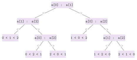
the tree is a comparison \(a[ i ] : a[ j ]\), its left subtree the
continuation when \(a[ i ] < a[ j ]\) and its right one the continuation
otherwise, and each leaf is the permutation \(\pi\) that the sort applies
when it gets there, i.e., the order \(a[ \pi_0 ] < a[ \pi_1 ] < \cdots <
a[ \pi_{n-1} ]\) that it has established.
Figure 12.1 shows the tree of insertionSort() on
three items. Since the \(n!\) orders of \(n\) distinct items need \(n!\)
different permutations to be undone, a correct sort has a tree with at
least \(n!\) leaves. With fewer, two inputs that need different
permutations reach the same leaf, and one of them comes out unsorted.
Figure 12.2 shows such a tree (that of figure 11.6
of Morin 2013), with four leaves for
the six orders of three items.
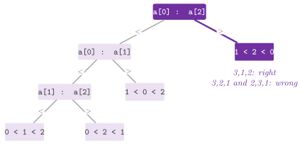
In passing, the tree of Figure 12.2 answers exercise 11.9 of Morin 2013: besides \(3 , 1 , 2\) and \(3 , 2 , 1\), which reach the same leaf and of which the second is sorted wrongly, the pair \(2 , 3 , 1\) and \(3 , 1 , 2\) reaches it too, and \(2 , 3 , 1\) comes out as \(3 , 1 , 2\). We now prove the two facts on binary trees on which the lower bound rests.
Lemma 12.1. A binary tree with \(k \ge 1\) leaves has height at least \(\log_2 k\).
Proof. A tree of height \(h\) has at most \(2^h\) leaves, by induction on \(h\): a tree of height 0 is a leaf, and the two subtrees of the root of a tree of height \(h > 0\) have height at most \(h - 1\), hence at most \(2^{h-1}\) leaves each. Thus \(k \le 2^h\), i.e., \(h \ge \log_2 k\). \(\square\)
Lemma 12.2. If a leaf of a binary tree with \(k \ge 1\) leaves is drawn uniformly at random, its expected depth is at least \(\log_2 k\).
Proof. We argue by induction on the height of the tree (not on \(k\), since a root with one child has a subtree with all the \(k\) leaves). For height 0 the tree is a leaf and the bound is 0. Otherwise let the subtrees of the root, of smaller height, have \(k_1\) and \(k_2\) leaves, \(k_1 + k_2 = k\) (one of them possibly empty). The leaf drawn lies in the first one with probability \(k_1 / k\), and is then a leaf drawn uniformly from it. Hence, by the inductive hypothesis applied to the nonempty subtrees, its expected depth \(E( k )\) satisfies
where the second inequality holds since \(x \log_2 x\) is convex, and therefore \(k_1 \log_2 k_1 + k_2 \log_2 k_2\) is least, for a fixed sum, at \(k_1 = k_2 = k / 2\) (a term with \(k_i = 0\) counts as 0). \(\square\)
The number of leaves we need is \(n!\), whose logarithm is estimated by an elementary argument (the formula of Stirling gives the sharper \(\log_2 n! = n \log_2 n - n \log_2 e + O( \log n )\)).
Lemma 12.3. For every \(n \ge 1\), \(n \log_2 n - n \log_2 e \le \log_2 n! \le n \log_2 n\). Hence \(\log_2 n! = n \log_2 n - O( n )\).
Proof. The upper bound holds since each of the \(n\) factors of \(n!\) is at most \(n\). For the lower one, \(e^n = \sum_{j \ge 0} n^j / j! \ge n^n / n!\), the term \(j = n\) of the series. Hence \(n! \ge ( n / e )^n\), and the logarithms give the claim. \(\square\)
Theorem 12.1. For any deterministic sort by comparisons and any \(n \ge 1\), there is an input of \(n\) distinct items on which the sort makes at least \(\lceil \log_2 n! \rceil \ge n \log_2 n - 1.443 \, n\) comparisons.
Proof. By correctness, the comparison tree of the sort has at least \(n!\) leaves, and hence, by Lemma 12.1, a leaf at depth at least \(\log_2 n!\) (an integer, the depth of a leaf is at least \(\lceil \log_2 n! \rceil\)). Some input reaches that leaf, and the sort makes on it as many comparisons as the depth; Lemma 12.3, with \(\log_2 e < 1.443\), gives the inequality. \(\square\)
A randomized sort, such as the quicksort with a random pivot, has no single tree, but it does not escape the bound either (Morin 2013, §11.1.4). We may regard it as a deterministic sort with two inputs, the items and a sequence \(b\) of random numbers from which it takes its choices. For each fixed \(b\) it is a deterministic sort with a tree \(\mathcal{T}( b )\), which, once the nodes that no input reaches are pruned, has exactly \(n!\) leaves (at least \(n!\) to be correct, and at most \(n!\) since each order of the items follows one path).
Theorem 12.2. For any sort by comparisons, deterministic or randomized, and any \(n \ge 1\), the expected number of comparisons on a random permutation of \(n\) distinct items is at least \(\log_2 n! = n \log_2 n - O( n )\).
Proof. We fix the random choices \(b\). A random permutation of the items reaches each of the \(n!\) leaves of \(\mathcal{T}( b )\) with probability \(1 / n!\), i.e., it draws a leaf uniformly, whose expected depth is at least \(\log_2 n!\) by Lemma 12.2. Since this holds for each \(b\), it holds for the expectation over \(b\) as well. \(\square\)
Hence merge sort and heapsort, with \(O( n \log n )\) comparisons in the worst case, and Quicksort on average, are optimal up to a constant factor (cf. (12.3) and (12.4) below). On a restricted input, the same argument gives finer bounds. If the input is known to consist of \(r\) runs of lengths \(\ell_1 , \ldots , \ell_r\), the possible outputs are the ways of interleaving them, \(n! / ( \ell_1 ! \cdots \ell_r ! )\), and the bound becomes
by Lemma 12.3 and \(\ell_i ! \le \ell_i^{\ell_i}\),
which give \(\log_2 n! - \sum_i \log_2 \ell_i ! \ge n \log_2 n - n \log_2 e -
\sum_i \ell_i \log_2 \ell_i = n H - n \log_2 e\). The bound is 0 on a sorted
input and \(\log_2 n!\) on \(n\) runs of one item, and both ends are met: the merge sorts of RunSorts.h meet (12.2) up to \(O( n )\)
(§12.5). Likewise, with \(k\) distinct keys, each
repeated \(n / k\) times, the bound is \(n \log_2 k - O( n )\), which the
three-way partitions meet up to the factor \(2 \ln 2 < 1.39\) (Theorem
12.6). Finally, the sorts by
digits escape the bound since a single step of theirs, the address
\(B[ \mathit{key} ]\) of an array of counts, has \(k\) outcomes instead of 2,
and their execution is therefore not a binary tree
(§12.10).
How close one can get to \(\lceil \log_2 n! \rceil\) is answered, for most
\(n\), by the merge insertion of Ford and Johnson
1959 (Knuth 1998,
§5.3.1), mergeInsertionSort() of
KnuthSorts.h (Algorithm 12.1). The items are paired
and the two items of each pair compared, and the larger items are sorted
recursively into a chain. The smaller ones are then inserted into the chain
by binary search, in the order given by the Jacobsthal numbers \(t_j = (
2^{j+1} + ( -1 )^j ) / 3\), i.e., \(1 , 3 , 5 , 11 , 21 , \ldots\). Indeed, the
items \(s_{t_j} , s_{t_j - 1} , \ldots , s_{t_{j-1} + 1}\) are inserted in
this order, each into a prefix of the chain of at most \(2^j - 1\) items
(those before its partner); each binary search thus costs \(j\) comparisons,
and none is wasted on a prefix that is not one less than a power of 2.
In ADS/sort/KnuthSorts.h, the functions are declared as
// declarations of <ADS/sort/KnuthSorts.h>
template< class T , class C = std::less<> >
void binaryInsertionSort( std::vector< T > & A , C less = C() );
template< class T , class C = std::less<> >
void listInsertionSort( std::vector< T > & A , C less = C() ,
                        std::size_t * moves = nullptr );
template< class T >
void addressCalculationSort( std::vector< T > & A , std::size_t M = 0 );
template< RadixKey T >
void radixExchangeSort( std::vector< T > & A );
template< class T , class C = std::less<> >
void tournamentSort( std::vector< T > & A , C less = C() );
template< class T , class C = std::less<> >
void mergeInsertionSort( std::vector< T > & A , C less = C() );
long fordJohnsonBound( std::size_t n );
Algorithm 12.1. The merge insertion of Ford and Johnson (Knuth 1998, §5.3.1).
Lemma 12.4. (Knuth 1998, §5.3.1.) The merge insertion makes at most
comparisons on \(n\) items. Moreover, \(F( n ) = n \log_2 n - \theta_n n + O( \log n )\) with \(1.329 < \theta_n < 1.415\), the value oscillating with the place of \(n\) between two powers of 2, and \(F( n ) = \lceil \log_2 n! \rceil\) for \(n \le 11\) and for \(n = 20 , 21\).
Proof. This count is equation (3) of Knuth 1998, §5.3.1, which holds for the order of the insertions described above, each binary search into a prefix of at most \(2^j - 1\) items; this is the order of Algorithm 12.1. Its asymptotics and the values of \(n\) for which it meets the bound are in the same section. \(\square\)
fordJohnsonBound() computes \(F( n )\), and the test taocp.knuth-sorts
checks that the sort makes at most \(F( n )\) comparisons. Against the \(n
\log_2 n - 1.443 \, n\) of Stirling, \(F( n )\) thus exceeds \(\log_2 n!\) by
between about \(0.028 \, n\) and \(0.114 \, n\) for large \(n\). Its bookkeeping
of the pairs and of the insertions makes the sort slow in time, however,
and it is of interest only when a comparison is far dearer than a move.
12.3 The elementary sorts and the inversions¶
The elementary sorts of Montresor 2025,
§2.7 keep a sorted prefix
\(A[ 0 .. i - 1 ]\) and extend it by one item at each step. Selection Sort
(selectionSort() of SelectionSort.h) appends the minimum of the rest,
swapping it with \(A[ i ]\), whatever the input
(Algorithm 12.2). Insertion Sort (insertionSort() of
InsertionSort.h) inserts \(A[ i ]\) in the prefix, as one sorts a hand of
cards, moving one place to the right the items larger than it. Its overload
on a range \([ \mathit{lo} , \mathit{hi} )\) is the base case of
all the hybrid sorts of the area, and insertionSortSentinel() first moves
the minimum to \(A[ 0 ]\), and its inner loop then needs no test of the left
end (Knuth 1998, §5.2.1).
In ADS/sort/SelectionSort.h, the functions are declared as
// declarations of <ADS/sort/SelectionSort.h>
template< class T , class C = std::less<> >
void selectionSort( std::vector< T > & A , C less = C() );
Algorithm 12.2. Selection Sort, Insertion Sort, and Insertion Sort with a sentinel (Montresor 2025, §2.7.1 and §2.7.2).
In ADS/sort/InsertionSort.h, the functions are declared as
// declarations of <ADS/sort/InsertionSort.h>
template< class T , class C = std::less<> >
void insertionSort( std::vector< T > & A , std::size_t lo , std::size_t hi ,
                    C less = C() );
template< class T , class C = std::less<> >
void insertionSort( std::vector< T > & A , C less = C() );
template< class T , class C = std::less<> >
void insertionSortSentinel( std::vector< T > & A , C less = C() );
Lemma 12.5. Selection Sort makes \(n ( n - 1 ) / 2\) comparisons and \(n - 1\) swaps on any input of \(n \ge 1\) items, and it is not stable.
Proof. At the step \(i\), for \(i = 0 , \ldots , n - 2\), Selection Sort finds the minimum of the \(n - i\) items of \(A[ i .. n - 1 ]\) with \(n - i - 1\) comparisons and makes one swap (possibly of \(A[ i ]\) with itself), and these sum to \(n ( n - 1 ) / 2\) and \(n - 1\). On \(2 , 2' , 1\) the first swap carries \(2\) past \(2'\), and the output is \(1 , 2' , 2\). \(\square\)
The cost of Insertion Sort, instead, depends on the input through its inversions.
Lemma 12.6. Insertion Sort makes exactly \(I( A )\) moves and at most \(I( A ) + n - 1\) comparisons; any sort that only swaps adjacent items makes at least \(I( A )\) swaps, and hence \(n ( n - 1 ) / 4\) on average over the permutations of distinct items.
Proof. The item \(A[ i ]\) moves past exactly the items of the prefix larger than it, i.e., the inversions \(( j , i )\) with \(j < i\), and each test of the inner loop but the last one is followed by a move. A swap of two adjacent items changes \(I( A )\) by exactly one, and a permutation and its reverse have together \(n ( n - 1 ) / 2\) inversions, since each pair is inverted in exactly one of the two; pairing each permutation with its reverse gives the average. \(\square\)
Note that Insertion Sort is thus \(\Theta( n )\) on an input with \(O( n )\)
inversions,
and \(\Theta( n^2 )\) on a reversed one. It is stable, since an item never
moves past an item equal to it, and with its simple loop it is usually the
fastest sort of a few items. Two variants of Knuth 1998,
§5.2.1 in KnuthSorts.h act on its two
costs (Algorithm 12.3). In binaryInsertionSort()
the place of \(A[ i ]\) is found by a binary search in the prefix. In
listInsertionSort() (Algorithm 5.2.1L of Knuth) each item is inserted into
a list of links \(L\) over the places, from the last item to the first, and no
item moves until the end, when the vector is rearranged once along the
list, which usually pays when the items are large.
Algorithm 12.3. The binary and the list insertion sorts (Knuth 1998, §5.2.1).
Lemma 12.7. binaryInsertionSort() makes
at most \(\sum_{k=1}^{n} \lceil \log_2 k \rceil \le \log_2 n! + n\)
comparisons and \(\Theta( n^2 )\) moves on average; listInsertionSort()
makes at most \(n ( n - 1 ) / 2\) comparisons and \(n\) moves. Both are
stable.
Proof. A binary search in a prefix of \(i\) items halves an interval of \(i + 1\) places, and hence it makes at most \(\lceil \log_2 ( i + 1 ) \rceil\) comparisons; summing over \(i = 1 , \ldots , n - 1\) gives the bound, and \(\lceil \log_2 k \rceil < \log_2 k + 1\). The insertion then moves the items of the prefix larger than \(A[ i ]\), i.e., \(I( A )\) in all, whose average is \(n ( n - 1 ) / 4\) by Lemma 12.6. The list insertion of the item \(j\) walks at most the \(n - 1 - j\) items already in the list, and the final pass moves each item once into a new vector. Since the binary search stops after the items equal to \(A[ i ]\), and the list insertion, from the right, puts the item \(j\) before the equal items that follow it in the input; both keep thus the order of the equal items. \(\square\)
The sorts by adjacent exchanges of ExchangeSorts.h are all bound by
Lemma 12.6 (Knuth 1998,
§5.2.2), and they are in the library for
what they teach, their speed being (arguably) of little interest. bubbleSort() makes
passes from left to right that swap the adjacent items out of order, each
pass ending at the last swap of the previous one. A small item near the end
(a turtle) moves one place to the left per pass; cocktailShakerSort()
alternates passes to the right and to the left, and a turtle thus reaches
the front in one pass. oddEvenSort(), the odd-even transposition sort of
Habermann 1972, compares the pairs \((
2 i , 2 i + 1 )\) and then the pairs \(( 2 i + 1 , 2 i + 2 )\) in turns; within
a phase the comparisons are independent, which makes it a sort for \(n\)
processors on a line, and the function can report the rounds of two phases
that it made. combSort() of Dobosiewicz
1980 compares the items at a gap
that shrinks by the factor \(1.3\) at each pass (\(g \gets \lfloor 10 g / 13
\rfloor\)), which moves the turtles far, and it ends as a bubble sort with gap
1; it is (reportedly) near \(O( n \log n )\) in practice. Finally,
gnomeSort() of Sarbazi-Azad 2000
moves one position right while the two items behind it are in order, and
swaps them and moves left otherwise, i.e., it is the insertion sort with
swaps and with no nested loop (Algorithm 12.4).
In ADS/sort/ExchangeSorts.h, the functions are declared as
// declarations of <ADS/sort/ExchangeSorts.h>
template< class T , class C = std::less<> >
void bubbleSort( std::vector< T > & A , C less = C() );
template< class T , class C = std::less<> >
void cocktailShakerSort( std::vector< T > & A , C less = C() );
template< class T , class C = std::less<> >
void oddEvenSort( std::vector< T > & A , C less = C() ,
                  std::size_t * rounds = nullptr );
template< class T , class C = std::less<> >
void combSort( std::vector< T > & A , C less = C() );
template< class T , class C = std::less<> >
void gnomeSort( std::vector< T > & A , C less = C() );
Algorithm 12.4. The sorts by adjacent exchanges, and the comb sort.
Lemma 12.8. On \(n\) items, bubbleSort()
and cocktailShakerSort() make \(I( A )\) swaps, at most \(n ( n - 1 ) / 2\)
comparisons, and \(n - 1\) on a sorted vector; gnomeSort() makes \(I( A )\)
swaps and at most \(2 I( A ) + n - 1\) comparisons; oddEvenSort() sorts
after \(n\) phases, i.e., \(\lceil n / 2 \rceil\) rounds, and stops after one
more; combSort() makes \(O( n^2 )\) comparisons. All but the comb sort are
stable.
Proof. Each of the first three swaps only adjacent items out of order, and
hence it removes one inversion per swap and ends with none (Lemma
12.6). A pass of bubbleSort() that ends with its
last swap at the place \(\mathit{last}\) leaves \(A[ \mathit{last} - 1 ] \le A[
\mathit{last} ]\) and, after it, the largest items in their places, since
the largest item met is carried to the end of the pass; the next pass may
thus stop at \(\mathit{last}\), and the passes compare \(n - 1 , n - 2 ,
\ldots\) items at most, \(n - 1\) in all on a sorted vector, whose first pass
makes no swap. As for cocktailShakerSort(), its passes to the left are the
mirror. A step of gnomeSort() at a place \(i > 0\) makes one comparison;
the steps back are the \(I( A )\) swaps, and the steps forward are \(n - 1\)
plus one for each step back, which must be retraced. For the odd-even transposition, the bound on the
phases is Theorem 1 of Habermann
1972 (cf. Knuth 1998, §5.3.4,
exercise 37). The comb sort makes
\(O( \log n )\) passes with a gap above 1 and then, by the argument of
bubbleSort(), at most \(n\) passes with gap 1, each of \(n\) comparisons at
most. Finally, an adjacent swap of two equal items never happens, since
the tests are strict, while the comb sort swaps items \(g\) places apart,
past the items between them: on \(2 , 2' , 1\), its first pass with gap 2
gives \(1 , 2' , 2\). \(\square\)
Shell Sort (shellSort() of ShellSort.h, Montresor 2025,
§15.1; Shell
1959) escapes the bound of
Lemma 12.6 by exchanging far items first. A pass
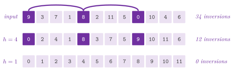
with gap \(h\) is an insertion sort of the \(h\) interleaved subsequences of
the places congruent modulo \(h\) (Algorithm 12.5),
and a single move at distance \(h\) may remove up to \(2 h - 1\) inversions.
The passes go through a decreasing sequence of gaps down to 1, and the last
pass, an insertion sort, usually finds few inversions;
Figure 12.3 shows two passes on twelve items. Montresor's
book sees it as a local search that lowers the inversions. One may ask why
the passes do not undo each other, and the following property answers it.
In ADS/sort/ShellSort.h, the functions are declared as
// declarations of <ADS/sort/ShellSort.h>
std::vector< std::size_t > knuthGaps( std::size_t n );
std::vector< std::size_t > shellGaps( std::size_t n );
std::vector< std::size_t > hibbardGaps( std::size_t n );
std::vector< std::size_t > prattGaps( std::size_t n );
std::vector< std::size_t > ciuraGaps( std::size_t n );
template< class T , class C = std::less<> >
void shellSort( std::vector< T > & A ,
                const std::vector< std::size_t > & gaps ,
                C less = C() );
template< class T , class C = std::less<> >
void shellSort( std::vector< T > & A , C less = C() );
Algorithm 12.5. Shell Sort on the gaps \(H\), and with the gaps of the book (Montresor 2025, §15.1).
Lemma 12.9. A vector that is \(h\)-sorted, i.e., with \(A[ i ] \le A[ i + h ]\) for each \(i\), stays \(h\)-sorted after a pass with gap \(g\).
Proof. This is Theorem K of Knuth 1998, §5.2.1, which rests on the following fact: if \(x_1 , \ldots , x_{m+r}\) and \(y_1 , \ldots , y_{s+r}\) satisfy \(x_j \le y_{s+j}\) for \(1 \le j \le r\), and \(x'\) and \(y'\) are the two sequences sorted, then \(x'_j \le y'_{s+j}\) for \(1 \le j \le r\). Indeed, the \(s + j\) smallest items of \(y\) (those of places \(1 , \ldots , s + j\) of \(y'\)) include at least \(j\) of \(y_{s+1} , \ldots , y_{s+r}\), since only \(s\) items lie outside them; each such \(y_{s+i}\) is at least \(x_i\), so that \(j\) distinct items of \(x\) are at most \(y'_{s+j}\), and hence so is \(x'_j\). Now let \(A\) be \(h\)-sorted, and take a place \(i\) with \(i + h < n\); let \(p_1 < \cdots < p_a\) be the places congruent to \(i\) modulo \(g\), and \(q_1 < \cdots < q_b\) those congruent to \(i + h\). The places \(p_k\) with \(p_k + h < n\) are a prefix \(p_1 , \ldots , p_r\), and since consecutive places of a class differ by \(g\), their images \(p_k + h\) are the last \(r\) places \(q_{s+1} , \ldots , q_{s+r}\) of the other class, \(s = b - r\). The fact, with \(x\) the items of the first class (the \(r\) constrained ones first) and \(y\) those of the second, shows that after the pass, which sorts each class, \(A[ p_k ] = x'_k \le y'_{s+k} = A[ p_k + h ]\) for each \(k \le r\), in particular at \(i\). \(\square\)
Its time depends on the gaps, which the five generators of the header give in
increasing order, from 1 (the contracts check both properties): knuthGaps(),
the \(h = ( 3^i - 1 ) / 2\) of the book, i.e., \(1 , 4 , 13 , 40 , 121 , \ldots\),
the default of shellSort( A ); shellGaps(), the \(\lfloor n / 2^j \rfloor\)
of Shell; hibbardGaps(), the \(2^k - 1\) of Hibbard
1963; prattGaps(), all the \(2^i 3^j\) up
to \(n\) (Pratt 1971); and ciuraGaps(),
\(1 , 4 , 10 , 23 , 57 , 132 , 301 , 701\) and then the factor \(2.25\), found by
experiment (Ciura 2001) and usually among
the fastest in practice, with no bound proved.
Lemma 12.10. (i) A vector that is 2-sorted and 3-sorted is sorted by one pass of insertion with gap 1 that moves each item one place at most; hence the gaps of Pratt sort in \(O( n \log^2 n )\) time. (ii) The gaps of Hibbard and those of the book take \(O( n^{3/2} )\) time in the worst case. (iii) The gaps of Shell take \(\Theta( n^2 )\) time in the worst case, for \(n\) a power of 2.
Proof. (i) In a vector 2-sorted and 3-sorted, \(A[ i ] \le A[ i + h ]\) for every \(h \ge 2\), since \(h\) is a sum of 2s and 3s; the only inversions are thus between neighbors, disjoint pairs, which the pass with gap 1 swaps. With the gaps of Pratt, the vector is \(2 h\)-sorted and \(3 h\)-sorted before the pass with gap \(h\) (by Lemma 12.9, the passes do not undo it), and that pass, on each of its \(h\) subsequences, moves each item one step at most, in \(O( n )\) time; there are \(O( \log^2 n )\) gaps \(2^i 3^j \le n\). (ii) For the gaps \(2^k - 1\) this is the theorem of Papernov and Stasevich in Knuth 1998, §5.2.1, whose proof rests on two consecutive gaps being coprime and growing by a bounded factor; the same section gives the same bound for the gaps \(( 3^i - 1 ) / 2\), for which \(h_{s+1} = 3 h_s + 1\) is coprime with \(h_s\) as well. (iii) With \(n = 2^t\), the gaps before the last are all even, and hence the items of the odd places are never compared with those of the even places until the last pass. If the \(n / 2\) larger items are at the even places and the smaller at the odd ones, the last pass finds the \(j\)-th smaller item, for \(j = 1 , \ldots , n / 2\), at the place \(2 j - 1\), after \(j\) larger items, i.e., \(\sum_j j > n^2 / 8\) inversions, which it removes one per move. \(\square\) With a single gap \(h > 1\) the vector ends only \(h\)-sorted, as in figure 15.4 of Montresor 2025. Shell Sort is in place and iterative, but not stable, which rather limits its use on records.
12.4 Merge sort¶
Merge Sort (mergeSort() of MergeSort.h, Montresor 2025,
§2.7.3; Morin 2013,
§11.1.1) is the classical example of
divide and conquer (§13.4): a part of at most
one item is sorted, and a larger part is split into two halves, which are
sorted recursively and then merged (Algorithm
12.6). The merge, mergeParts(), the Merge() of the
book, writes into a vector \(B\) allocated once by mergeSort() the smaller
of the first items of the two halves, until one of them runs out, and then
copies the merged items back. Both call the recursion, mergeSortRec():
// declarations of <ADS/sort/MergeSort.h>
template< class T , class C = std::less<> >
void mergeParts( std::vector< T > & A , std::vector< T > & B ,
                 std::size_t start ,
                 std::size_t mid , std::size_t end , C less = C() ,
                 long long * inv = nullptr );
template< class T , class C = std::less<> >
void mergeSort( std::vector< T > & A , std::size_t cutoff = 1 , C less = C() );
template< class T , class C = std::less<> >
void mergeSort( List< T > & L , C less = C() );
template< class T , class C = std::less<> >
void mergeSortBottomUp( std::vector< T > & A , C less = C() );
template< class T , class C = std::less<> >
long long countInversions( std::vector< T > & A , C less = C() );
template< class T , class C = std::less<> >
void mergeSortRec( std::vector< T > & A , std::vector< T > & B ,
                   std::size_t start , std::size_t end , std::size_t cutoff ,
                   C less = C() , long long * inv = nullptr );
Algorithm 12.6. Merge Sort and its merge
(Montresor 2025, §2.7.3), with the
cutoff of section 2.8. The counter \(\mathit{inv}\) is used by
countInversions() only.
Its code follows the pseudocode. We remark that the test is !
less( A[ j ] , A[ i ] ): an item of the left half goes first
when the two are equal, which makes the merge, and hence the sort, stable,
and that the items are moved, not copied.
When the right half runs out first, the rest of the left one is copied to \(B\).
When the left one does, the rest of the right one is already in its place, and
the copy back stops at \(k\). With a cutoff larger than 1,
mergeSort( A , cutoff ) sorts the parts of at most \(\mathit{cutoff}\) items
by insertionSort(), which is faster on few items (Montresor 2025,
§2.8), and it skips the merge of two
halves already in order, \(A[ \mathit{mid} ] \le A[ \mathit{mid} + 1 ]\), which
makes a sorted input cost \(O( n )\) (Lemma 12.13
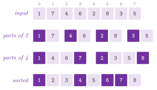
below). With the default cutoff 1 it is the plain sort of the book. Figure
12.4 shows the sort on the vector of exercise 11.1 of
Morin 2013.
Lemma 12.11. The merge of two sorted parts of \(n_1\) and \(n_2\) items makes at most \(n_1 + n_2 - 1\) comparisons, and gives their items sorted, the equal items of the left part before those of the right one.
Proof. Each comparison writes one item to \(B\), and after the comparison that writes the last item of one part no comparison is made. Hence at most \(n_1 + n_2 - 1\) comparisons. The item written is the smaller of the two first items, i.e., the least item not yet written, since each part is sorted, and on a tie it is the left one. \(\square\)
Theorem 12.3. mergeSort() sorts \(n\) items
in \(O( n \log n )\) time with at most \(n \log_2 n\) comparisons; more
precisely, with at most
Proof. By Lemma 12.11, the worst case satisfies \(C( 1 ) = 0\) and \(C( n ) \le C( \lceil n / 2 \rceil ) + C( \lfloor n / 2 \rfloor ) + n - 1\). We show \(C( n ) \le n \log_2 n\) by induction, as in Morin 2013, §11.1.1. For \(n\) even, \(C( n ) \le n - 1 + 2 ( n / 2 ) \log_2 ( n / 2 ) = n \log_2 n - 1\). For \(n\) odd, with \(m = n / 2\), the two halves have \(m + 1 / 2\) and \(m - 1 / 2\) items, and
where we used \(\log_2 ( m + 1 / 2 ) + \log_2 ( m - 1 / 2 ) \le 2 \log_2 m\) (the concavity of the logarithm). Here the last term is at most \(1 / 2\), since \(m + 1 / 2 \le 2 ( m - 1 / 2 )\) for \(m \ge 3 / 2\), and therefore \(C( n ) < n + n ( \log_2 n - 1 ) = n \log_2 n\). The exact solution (12.3) of the recurrence with equality, which is attained (each merge can be made to compare up to the last item), is in Knuth 1998, §5.2.4. As for the time, it is \(O( 1 )\) per comparison and per move, and each level of the recursion moves each item twice. \(\square\)
Indeed, the same bound follows from the tree of the recursion (Morin 2013, §11.1.1): for \(n\) a power of 2, the level \(i\) of the tree has \(2^i\) parts of \(n / 2^i\) items, whose merges cost \(O( n )\) in all, and there are \(\log_2 n\) levels. In Figure 12.4 each row is a level. The bound (12.3) is close to the lower bound of Theorem 12.1, at the price of a buffer of \(n\) items, which the next sorts avoid.
Lemma 12.12. The bound (12.3) exceeds \(\log_2 n!\) by less than \(( \log_2 e - 1 ) n + 1 < 0.443 \, n + 1\) when \(n\) is a power of 2, and by less than \(0.529 \, n + 1\) for any \(n \ge 1\).
Proof. Let \(2^{\lceil \log_2 n \rceil} = n 2^\theta\), \(0 \le \theta < 1\). Then (12.3) is \(n \log_2 n - n ( 2^\theta - \theta ) + 1\), and by Lemma 12.3 the excess is less than \(n ( \log_2 e - 2^\theta + \theta ) + 1\). For \(n\) a power of 2, \(\theta = 0\); in general, the convex function \(2^\theta - \theta\) is least at \(\theta = \log_2 \log_2 e\), where it is \(\log_2 e - \log_2 \log_2 e > 1 - 0.0861\), and \(\log_2 e - 1 + 0.0861 < 0.529\). \(\square\)
Three more functions of the header reuse the merge (Algorithm
12.7). The bottom-up sort, mergeSortBottomUp(), merges
the runs of lengths \(1 , 2 , 4 , \ldots\) with no recursion and no stack
(exercise 12.5 of Montresor 2025). The
overload mergeSort( L ) sorts a List with pointers (exercise 12.1 of the
book) only through the operations of the SEQUENCE: its second half is moved
into a list \(R\), both halves are sorted, and the items of \(R\) are inserted
into \(L\) at their places, since the abstract data type moves no cells between
lists. The merge sort of a list that relinks its cells instead, with no
auxiliary array (exercise 11.2 of Morin
2013), is listSort() of ListSort.h, in
Chapter 2, which merges the natural runs of the list as
a binary counter. countInversions() counts the pairs \(i < j\) with
\(A[ i ] > A[ j ]\) (exercise 12.3 of the book) as a side effect of the merges,
by the next lemma.
Algorithm 12.7. The merge sort from the bottom up, the merge sort of a list, and the count of the inversions (Montresor 2025, exercises 12.1, 12.3 and 12.5).
Lemma 12.13. With a cutoff \(c > 1\),
mergeSort( A , c ) sorts a sorted vector in \(O( c n )\) time.
mergeSortBottomUp() makes, for \(n\) a power of 2, the merges and the
comparisons of the recursive sort, and at most
\(( n - 1 ) \lceil \log_2 n \rceil\) comparisons for any \(n\). mergeSort( L )
sorts a list of \(n\) items in \(O( n \log n )\) time with \(n\) copies of items per
level of the recursion.
Proof. On a sorted vector each insertion sort of a part of at most \(c\) items
makes fewer than \(c\) comparisons and no move, and each merge is skipped after
one comparison; the parts and the merges are \(O( n )\). For \(n = 2^t\), the
passes of the bottom-up sort merge the same parts as the levels of the
recursion, the pass of the runs of length \(2^i\) the level \(t - i - 1\). For any
\(n\), the runs double in length at each pass, and hence there are
\(\lceil \log_2 n \rceil\) passes, each of at most \(n - 1\) comparisons by Lemma
12.11. Finally, a call of mergeSort( L ) on \(m\) items
moves its \(\lfloor m / 2 \rfloor\) last items into \(R\) and back into \(L\), and
the merge walks the two lists once, i.e., \(O( m )\) time and \(m\) copies at
most; the recursion has \(\lceil \log_2 n \rceil\) levels, whose parts cover the
\(n\) items. \(\square\)
Lemma 12.14. The number of inversions of a
vector is the sum, over the merges of mergeSort() with cutoff 1, of
\(\mathit{mid} - i + 1\) at each step that takes \(A[ j ]\) from the right
part. Hence countInversions() takes \(O( n \log n )\) time.
Proof. Each inversion \(( p , q )\), \(p < q\), has its two items in the two halves of exactly one merge, the one of the smallest part that contains both. Below it, the merges keep the items within their halves. In that merge, when the item of \(q\) is taken from the right part, the items still in the left part are exactly those larger than it (the smaller or equal ones were taken before it), i.e., \(\mathit{mid} - i + 1\) items, each of which forms an inversion with it. \(\square\)
The strand sort of StrandSort.h, strandSort( L , less , strands ), which
counts the strands in *strands if given (Knuth 1998,
§5.2.4, exercise 12) is a variant of
the natural merge sort on a List: a strand, i.e., the first item and
every later one not smaller than the last item taken, is pulled out of the
list and merged with the result, until the list is empty
(Algorithm 12.8).
In ADS/sort/StrandSort.h, the functions are declared as
// declarations of <ADS/sort/StrandSort.h>
template< class T , class C = std::less<> >
void strandSort( List< T > & L , C less = C() ,
                 std::size_t * strands = nullptr );
Algorithm 12.8. The strand sort.
Lemma 12.15. The strand sort of a list of \(n\) items makes \(s\) strands, \(s\) the length of a longest strictly decreasing subsequence, and takes \(O( s n )\) time, i.e., \(O( n )\) on a sorted list and \(\Theta( n^2 )\) on a strictly decreasing one; it is stable.
Proof. A strand, being non-decreasing, takes at most one item of a strictly decreasing subsequence, and hence \(s\) strands at least are made. Conversely, an item of the \(i\)-th strand, \(i > 1\), was left out of the \(( i - 1 )\)-th by a larger item before it, which belongs to that strand; going back strand by strand gives a strictly decreasing subsequence of \(i\) items, and hence \(s\) strands at most. Pulling a strand and merging it into the result cost \(O( n )\) each. On a tie the result goes first, and its items came earlier in the input than those of the strand, since each strand takes the first item left. \(\square\)
12.5 Natural merge sorts and runs¶
A natural merge sort merges the runs that the input already has, instead of the halves of a recursion, and the order of its merges decides its cost. Merging two adjacent runs costs (roughly) their total length. Hence a sequence of merges is a binary tree over the runs whose cost is the sum of \(\ell_i \cdot \mathrm{depth}( i )\), as for the codes of Huffman (§21.2), and the best such tree among those that keep the runs in their order, an optimal alphabetic tree, costs between \(n H\) and \(n H + 2 n\) (Mehlhorn 1975). Yet the \(2 n\) cannot be lowered much: on three runs of lengths \(\varepsilon n\), \(( 1 - 2 \varepsilon ) n\) and \(\varepsilon n\), either order of the two merges costs \(( 1 - \varepsilon ) n + n = ( 2 - \varepsilon ) n\), while \(n H\) tends to 0 with \(\varepsilon\). Timsort (Peters 2002) keeps the runs on a stack whose lengths grow from the top at least as the numbers of Fibonacci, merging when the rule fails. Hence the stack has \(O( \log n )\) runs, and its merges cost \(O( n + n H )\) comparisons (Auger et al. 2018).
powerSort() of RunSorts.h, the Powersort of Munro and Wild
2018 (the sort of Python from version
3.11), merges instead along a tree that is nearly the one of the midpoints
of the runs (Algorithm 12.9). A run is a maximal
non-decreasing stretch, or a strictly decreasing one, which is reversed
(strictly, so that the reversal keeps the sort stable). A run shorter than
\(\mathit{minrun} = 24\) items is extended to 24 items by a binary insertion
sort, and the merges thus start from runs long enough. The boundary between
two adjacent runs \([ s_1 , s_2 )\) and \([ s_2 , e_2 )\) has a power, the
first bit in which the midpoints of the two runs, as fractions of \(n\),
differ. Here nodePower() computes it from twice the midpoints, one
bit at a time:
In ADS/sort/RunSorts.h, the functions are declared as
// declarations of <ADS/sort/RunSorts.h>
template< class T , class C = std::less<> >
void powerSort( std::vector< T > & A , C less = C() ,
                std::size_t * runs = nullptr );
Here \(l / 2 n\) and \(r / 2 n\) are the two midpoints, and the test of line 3 compares their \(( k + 1 )\)-th bits.
Lemma 12.16. nodePower() returns the
first bit in which the two midpoints differ, after at most \(\lceil \log_2 n
\rceil + 1\) steps.
Proof. After the first \(k\) bits have been removed by lines 4 and 5, the \(( k + 1 )\)-th bits of the two midpoints are \([ l \ge n ]\) and \([ r \ge n ]\), which the test of line 3 compares. The loop keeps \(0 \le l < r < 2 n\), and each step doubles \(r - l\) (the subtraction of line 4 leaves it unchanged); since the two bits differ as soon as \(r - l \ge n\), and \(r - l \ge 1\) at the start, the loop ends after at most \(\lceil \log_2 n \rceil + 1\) steps. \(\square\)
The runs wait on a stack whose powers increase upwards, and a new boundary first merges the runs on the stack whose power is larger than its own. Hence the merges happen in the order of a post-order visit of the tree in which the boundary of power \(p\) is a node of depth \(p\), i.e., the tree that splits \([ 0 , 1 )\) at its midpoint, then each half at its midpoint, and so on, with the runs as its leaves. Table 12.3 follows the stack on five runs.
Algorithm 12.9. Powersort (Munro and Wild 2018).
Table 12.3. powerSort() on \(n = 16\) items
in five runs, \([ 0 , 5 )\), \([ 5 , 8 )\), \([ 8 , 10 )\), \([ 10 , 14 )\) and
\([ 14 , 16 )\) (as if no run were extended): the power of each boundary, the
merges it causes, and the stack after it (each entry a run and the power of
its right boundary).
| Boundary | Power | Merges | Stack after it |
|---|---|---|---|
| 5 | 2 | \([ 0 , 5 ) / 2\) | |
| 8 | 1 | \([ 0 , 5 ) + [ 5 , 8 )\) | \([ 0 , 8 ) / 1\) |
| 10 | 2 | \([ 0 , 8 ) / 1\), \([ 8 , 10 ) / 2\) | |
| 14 | 3 | \([ 0 , 8 ) / 1\), \([ 8 , 10 ) / 2\), \([ 10 , 14 ) / 3\) | |
| end | \([ 10 , 14 ) + [ 14 , 16 )\), then \([ 8 , 10 ) + [ 10 , 16 )\), then \([ 0 , 8 ) + [ 8 , 16 )\) |
Theorem 12.4. (Munro and Wild) The merges of Powersort on \(r\) runs of lengths \(\ell_1 , \ldots , \ell_r\) cost at most \(n H + 2 n\), where the cost of a merge is the total length of the two runs. The stack never holds more than \(\lceil \log_2 n \rceil + 1\) runs.
Proof. We follow Munro and Wild 2018, taking from them one fact on the tree of the merges, which is the Cartesian tree of the powers of the \(r - 1\) boundaries (the root the boundary of least power, merged last): the powers strictly increase along each path from the root, so that a run lies at depth at most the larger power \(p_i\) of its two boundaries. The midpoints of two adjacent runs, as fractions of \(n\), differ by at least \(\ell_i / ( 2 n )\) for each of the two runs, and two numbers of \([ 0 , 1 )\) that differ by \(\delta\) differ in one of their first \(\lfloor \log_2 ( 1 / \delta ) \rfloor + 1\) bits; hence \(p_i \le \lfloor \log_2 ( n / \ell_i ) \rfloor + 2\). Each merge costs the lengths of the runs below it, so that the total cost is \(\sum_i \ell_i \, \mathrm{depth}( i ) \le \sum_i \ell_i ( \log_2 ( n / \ell_i ) + 2 ) = n H + 2 n\). As for the stack, a boundary is pushed only after the merges of the runs whose boundary has a larger power, and two boundaries adjacent on the stack never have the same power (the second fact we take from the paper), so that the powers strictly increase upwards; they lie between 1 and \(\lfloor \log_2 n \rfloor + 1\), since two adjacent runs of at least one item have midpoints at least \(1 / n\) apart, and the stack holds therefore at most \(\lfloor \log_2 n \rfloor + 1 \le \lceil \log_2 n \rceil + 1\) runs. The runs here are those after the extension to \(\mathit{minrun}\), whose binary insertion sorts cost \(O( n \log \mathit{minrun} ) = O( n )\) more. \(\square\)
With (12.2), Theorem 12.4 makes Powersort optimal up
to \(O( n )\) comparisons on any distribution of runs: \(O( n )\) on few
runs, and \(O( n \log n )\) always. A merge of RunSorts.h is engineered in
the ways of Timsort (Peters 2002). It
first skips the items of the left run already before the first item of the
right one, and those of the right run already after the last item of the
left one, both by galloping, an exponential search followed by a binary
one, and it rotates the two runs if the right one comes all before the left
one. It then merges with a buffer of the shorter run, from the front if it
is the left one and from the back otherwise; the buffer, made once, holds at
most half of the items. It switches to galloping when one run wins
7 times in a row, as McIlroy 1993
proposed, the threshold dropping by one at each gallop that pays and rising
by two at each one that does not. Two runs one after the other then merge in \(O( \log n )\) comparisons,
since the two gallops find at once that one run comes all before the
other; any two runs merge in \(O( n )\) comparisons, since a gallop that skips \(k\)
items, an exponential and a binary search, costs \(O( 1 + \log ( k + 1 ) )
= O( 1 + k )\) comparisons. Also, on the
arithmetic types, two runs that both come from runs extended to
\(\mathit{minrun}\), i.e., from an input in disorder whose merge no branch
predictor guesses, merge with no branch on the order (a conditional move and
two increments), and with the natural order they do not gallop, whose steps
cost more than the comparisons they save. On an input with long runs,
instead, the merges keep the branches, which follow its patterns. In Chapter 2, the plain natural merge
sort is naturalMergeSort() of SequenceAlgorithms.h, in
Chapter 2.
12.6 Quicksort¶
Quicksort (Hoare 1962; Montresor 2025,
§12.2; Morin 2013,
§11.1.2) is the other classical sort by
divide and conquer, which does its work before the recursion instead of
after it: partition(), the perno() of the book, rearranges
\(A[ \mathit{start} .. \mathit{end} ]\) around the pivot \(x = A[
\mathit{start} ]\), with the items before the final place \(j\) of
\(x\) are smaller than it and those after it are not, and the two parts are
then sorted recursively (Algorithm 12.10). It scans
the part once, keeping \(A[ \mathit{start} + 1 .. j ]\) the
items smaller than \(x\) seen so far. Each smaller item is swapped to the
place \(j + 1\).
In ADS/sort/QuickSort.h, the functions are declared as
// declarations of <ADS/sort/QuickSort.h>
template< class T , class C = std::less<> >
std::size_t partition( std::vector< T > & A , std::size_t start ,
                       std::size_t end , C less = C() );
template< class T , class C = std::less<> >
void quickSort( std::vector< T > & A , std::size_t start , std::size_t end ,
                C less = C() );
template< class T , class C = std::less<> >
void quickSort( std::vector< T > & A , C less = C() );
template< class T , class C = std::less<> >
void quickSort( List< T > & L , C less = C() );
template< class T , class C = std::less<> >
void quickSortTuned( std::vector< T > & A , std::size_t cutoff = 16 ,
                     C less = C() , std::size_t * depth = nullptr );
template< class T , class C = std::less<> >
std::size_t partitionByValue( std::vector< T > & A , std::size_t start ,
                              std::size_t end , const T & x , C less = C() );
Algorithm 12.10. The partition and Quicksort (Montresor 2025, §12.2).
Lemma 12.17. partition() makes
\(\mathit{end} - \mathit{start}\) comparisons and returns the place \(j\) of
the pivot, with \(A[ i ] < x\) for \(\mathit{start} \le i < j\) and
\(A[ i ] \ge x\) for \(j < i \le \mathit{end}\).
Proof. Each item but the pivot is compared once. Before the iteration of \(i\), the items of \(A[ \mathit{start} + 1 .. j ]\) are smaller than \(x\) and those of \(A[ j + 1 .. i - 1 ]\) are not: an item smaller than \(x\) is swapped with the first of the latter, which keeps both. At the end the pivot and \(A[ j ]\) change places. \(\square\)
Table 12.4 follows quickSort() on the vector of
exercise 11.1 of Morin 2013, whose first
item is its minimum: the first partition separates the pivot alone, a
foretaste of the worst case discussed below.
Table 12.4. quickSort() on
\(1 , 7 , 4 , 6 , 2 , 8 , 3 , 5\) (exercise 11.1 of Morin
2013): each call on a part of at least
two items, its pivot, the part after the partition and the place \(j\) of the
pivot; 7 + 6 + 4 + 2 = 19 comparisons in all.
| Call | Pivot | Part after partition() |
\(j\) |
|---|---|---|---|
quickSort(A, 0, 7) |
1 | 1 7 4 6 2 8 3 5 |
0 |
quickSort(A, 1, 7) |
7 | 5 4 6 2 3 7 8 |
6 |
quickSort(A, 1, 5) |
5 | 3 4 2 5 6 |
4 |
quickSort(A, 1, 3) |
3 | 2 3 4 |
2 |
A partition costs \(n - 1\) comparisons on a part of \(n\) items, and the two sides may have anything from 0 to \(n - 1\) items. On average, however, the pivot falls "near" the middle, as we now show. The analysis of Morin 2013, §11.1.2 rests on the correspondence with the random binary search trees of Chapter 8: on distinct items, the tree of the recursion of a quicksort whose pivot is equally likely to be any item of its part is a random binary search tree, the pivot of a part being the root of its subtree.
Lemma 12.18. Let the pivot of each part be equally likely to be any of its items, e.g., with a pivot drawn at random, or on a random permutation of distinct items. Then the items of ranks \(i < j\) are compared with probability \(2 / ( j - i + 1 )\), and the item of rank \(i\) (\(0 \le i < n\)) is compared in expectation \(2 ( H_{i+1} + H_{n-i} - 2 ) < 2 ( H_{i+1} + H_{n-i} )\) times.
Proof. Two items are compared only when one of them is the pivot of a
part that holds both, and then they are separated (or the pivot leaves).
Hence the items of ranks \(i < j\) are compared if and only if the first
pivot drawn among the ranks \(i , i + 1 , \ldots , j\) is one of the two,
since a pivot strictly between them separates them before. Up to that
moment the \(j - i + 1\) items stay in one part, and each of them is equally
likely to be the first pivot among them. This gives \(2 / ( j - i + 1 )\).
On a random permutation the parts left by partition() are again random
permutations of their items, since the partition looks at the items only
through their comparisons with the pivot (Sedgewick
1978), and the pivot of each part is
therefore equally likely to be any of its items. Summing over the partners
\(j \neq i\), the item of rank \(i\) has \(\sum_{d=2}^{i+1} 2 / d +
\sum_{d=2}^{n-i} 2 / d = 2 ( H_{i+1} - 1 ) + 2 ( H_{n-i} - 1 )\).
\(\square\)
Theorem 12.5. Under the hypothesis of
Lemma 12.18, quickSort() makes in expectation
comparisons, i.e., at most \(2 n \ln n + O( n )\), in \(O( n \log n )\) expected time.
Proof. By Lemma 12.18 and the linearity of the expectation, \(C( n ) = \sum_{i<j} 2 / ( j - i + 1 ) = \sum_{d=2}^{n} 2 ( n - d + 1 ) / d = 2 ( n + 1 ) ( H_n - 1 ) - 2 ( n - 1 ) = 2 ( n + 1 ) H_n - 4 n\). Equivalently, the pivot is the \(( j + 1 )\)-th smallest item with probability \(1 / n\) and leaves sides of \(j\) and \(n - 1 - j\) items, which gives the recurrence of (12.4); subtracting the recurrence of \(n - 1\) multiplied by \(n - 1\) from that of \(n\) multiplied by \(n\) gives \(n C( n ) = ( n + 1 ) C( n - 1 ) + 2 ( n - 1 )\), and dividing by \(n ( n + 1 )\) telescopes to the closed form. Since \(H_n = \ln n + O( 1 )\) and \(2 \ln n = ( 2 \ln 2 ) \log_2 n\), with \(2 \ln 2 < 1.3863\), the approximation follows. \(\square\)
The constant of (12.4) is about 39% above the \(n \log_2 n\) of Theorem 12.1, and the merge sort of Theorem 12.3 makes fewer comparisons; yet, Quicksort is in place and its inner loop is a scan, which usually (but not always) makes it faster in time. Its worst case, however, is quadratic.
Lemma 12.19. On a sorted vector of \(n\)
items, and on a vector of \(n\) equal items (exercise 12.4 of Montresor
2025), quickSort() makes \(n ( n - 1
) / 2\) comparisons and a recursion \(n - 1\) calls deep.
Proof. In both cases the pivot \(A[ \mathit{start} ]\) is not larger than
any item of its part, and hence partition() finds no item smaller than
it and leaves it in its place (cf. Lemma 12.17). The
call on \(m\) items thus makes \(m - 1\) comparisons and one call on the \(m - 1\)
items after the pivot, which are again sorted, or equal; summing over \(m = n
, \ldots , 2\) gives the claim. \(\square\)
This recursion is held by the stack of the program.
The count of the quicksort of Morin 2013, §11.1.2 differs from (12.4) in a detail: its partition in three compares the \(k\) items of a part with the pivot, the pivot included, and it returns at once on the parts of at most one item. Exercise 11.7 there proposes as its expectation \(2 n H_n - n + H_n\), which is not right, as the next lemma shows.
Lemma 12.20. On \(n \ge 2\) distinct keys, the quicksort of Morin 2013, with a random pivot, makes in expectation
comparisons.
Proof. \(T( n ) = n + ( 2 / n ) \sum_{k<n} T( k )\) with \(T( 0 ) = T( 1 ) = 0\), which is the recurrence of (12.4) plus one comparison per part of at least two items. Those with at least one item are one per item (each item is a pivot or a part of one item), \(n\) in all, and they are the nodes of a random binary search tree, whose leaves, the parts of one item, are \(( n + 1 ) / 3\) in expectation for \(n \ge 2\). Hence the extra comparisons are \(n - ( n + 1 ) / 3 = ( 2 n - 1 ) / 3\). \(\square\)
At \(n = 2\) both counts are exact, 2 for (12.5) and 1 for (12.4), while
\(2 n H_n - n + H_n\) gives 5.5. In the library, the test
ods_ints.ods.ex11.7.quicksort-expectation checks (12.5) on the recurrence
up to \(n = 2000\) and against the average of 4000 runs of that quicksort.
With equal keys, the same analysis gives the theorem of Morin 2013,
§11.1.2: a pivot that has duplicates takes
them all out of both sides, and equal keys can thus only lower the count.
Theorem 12.6. A quicksort with a pivot drawn uniformly at random and a partition in three (the items smaller than, equal to and larger than the pivot), counting one comparison for the test of an item against the pivot, makes in expectation at most \(n + 2 n \ln k \le n + 2 n \ln n\) comparisons on \(n\) items with \(k\) distinct keys.
Proof. We number the distinct keys \(1 , \ldots , k\), of multiplicities \(m_1 , \ldots , m_k\), and we let \(M[ a , b ]\) be the items of keys from \(a\) to \(b\). An item \(x\) of key \(a\) is compared only with pivots, at most once with each, and with at most one pivot of each key, since a pivot takes out of the recursion all the items equal to it. The items of keys from \(a\) to \(b > a\) stay in one part until the first pivot among them is drawn, and each of them is equally likely to be that pivot; hence \(x\) meets a pivot of key \(b\) with probability \(m_b / M[ a , b ] \le \ln ( M[ a , b ] / M[ a , b - 1 ] )\) (since \(t \le - \ln ( 1 - t )\)), and the same holds for \(b < a\). Summing over \(b > a\) the logarithms telescope to \(\ln ( M[ a , k ] / m_a ) \le \ln ( n / m_a )\), and likewise over \(b < a\); with the pivot of key \(a\), \(x\) is compared at most \(1 + 2 \ln ( n / m_a )\) times in expectation. Over the \(n\) items this is \(n + 2 n \sum_a ( m_a / n ) \ln ( n / m_a )\), and the entropy of the multiplicities is at most \(\ln k\). \(\square\)
On distinct keys the bound is that of (12.4) up to \(O( n )\), and with
\(k = O( 1 )\) keys it is linear. threeWayQuickSort()
(§12.7) draws its pivot by a generator of fixed seed,
so that the sort is the same on each run, and it leaves the parts of at
most 16 items to insertionSort().
Lemma 12.21. On an input of \(n\) items with
\(k\) distinct keys, chosen independently of the generator, threeWayQuickSort()
makes at most \(4 n \ln k + O( n )\) calls of less in expectation.
Proof. Its partition calls less once for an item smaller than the pivot
and twice for the others, i.e., at most twice per test of Theorem
12.6, whose bound \(n + 2 n \ln k\) holds for the
partitions above the cutoff, since the parts of at most 16 items only cut
the recursion short. As for the insertion sorts of these parts, which are disjoint,
make \(O( 16 n ) = O( n )\) calls. \(\square\)
More variants of QuickSort.h complete the section of the book (Algorithm
12.11). In quickSortTuned() the improvements of the
section are combined. Its pivot is the median of \(A[ \mathit{start} ]\), \(A[ \lfloor
( \mathit{start} + \mathit{end} ) / 2 \rfloor ]\) and \(A[ \mathit{end} ]\), and
the partition of Hoare 1962 scans from
both ends, swapping the pairs on the wrong sides, and stops on the items
equal to the pivot. Parts of at most \(\mathit{cutoff}\) items (16 by default,
3 at least) are left to insertionSort(), and the recursion is an explicit
stack that holds the larger part while the smaller one is sorted.
Lemma 12.22. The stack of quickSortTuned()
never holds more than \(\lfloor \log_2 n \rfloor\) parts, and a vector of \(n\)
equal items costs it \(O( n \log n )\) time. On a random permutation of
distinct items, the median of three gives \(\frac{12}{7} n \ln n + O( n )\)
comparisons in expectation, about \(1.188 \, n \log_2 n\).
Proof. When the stack holds \(s\) parts, the part being sorted has at most
\(n / 2^s\) items, since each push keeps the smaller part, of at most half the
items of the part split; a push needs more than 3 items, and hence
\(s \le \lfloor \log_2 n \rfloor\). On equal items both scans stop at every
item, and they meet in the middle of the part, where the pivot goes; the parts
halve, which gives \(T( n ) = 2 T( n / 2 ) + O( n )\). The constant of the
median of three is that of Sedgewick
1978 (cf. Knuth 1998,
§5.2.2), under the hypothesis of Lemma
12.18 on the parts. \(\square\) Also,
partitionByValue() partitions by a value \(x\) not necessarily in the part,
the items not larger than \(x\) first, and returns how many they are. Finally,
quickSort( L ) sorts a List by moving its items into three lists, smaller,
equal and larger than the pivot, which it concatenates after the two recursive
sorts (exercise 12.1 of Montresor
2025).
Algorithm 12.11. The tuned Quicksort, the partition by a value, and the Quicksort of a list (Montresor 2025, §12.2 and exercise 12.1).
Every deterministic rule for the pivot has its killer inputs: the sorted
vector for the first item (exercise 11.3 of Morin
2013), and an input built by the
adversary below for the middle item (exercise 11.4) or for any rule that
does not look at the values (exercise 11.5). The adversary of McIlroy
1999, QuicksortAdversary of
QuicksortAdversary.h, goes further: it is a comparator of the items
\(0 , \ldots , n - 1\) that gives them their values while the sort runs, and
it defeats also the quicksorts with a random pivot, since it answers after
the draw (exercise 11.6). Every item starts as gas, larger than every
value given. When two gas items are compared, one of them is frozen to the
next value, the smallest still free, and the adversary prefers to freeze the
item that was last compared with a frozen one, i.e., the candidate for the
pivot, since a quicksort compares its pivot with all the other items of its
part (Algorithm 12.12).
The public members of QuicksortAdversary are
// declarations of <ADS/sort/QuicksortAdversary.h>
class QuicksortAdversary
{
 public:
 explicit QuicksortAdversary( std::size_t n );
 class Less;  // the comparator of the adversary
 Less less( void );
 std::vector< std::size_t > items( void ) const;
 std::size_t comparisons( void ) const;
 std::vector< std::size_t > input( void ) const;
 };
Algorithm 12.12. The comparator of the adversary (McIlroy 1999); \(v[ x ]\) is the value of the item \(x\), \(\infty\) for the gas, and \(c\) the candidate for the pivot.
QuicksortAdversary gives the comparator by less(), of type
QuicksortAdversary::Less, and the items to sort by items(). One may read
the comparisons made so far by comparisons(), and, at the end, the values
given by input(), the gas left being frozen in order.
Lemma 12.23. For any quicksort that takes
its pivot among \(O( 1 )\) items of its part, deterministically or at random,
the comparator of the adversary makes it do \(\Theta( n^2 )\) comparisons
on \(n\) items, at least \(\binom{n}{2}\) when the partition compares the pivot
once with each other item of its part; and the values that input()
gives are an input on which a
deterministic such sort makes the same comparisons.
Proof. The pivot of a part is compared with the other items of the part. At the first comparison of the partition between two gas items, the candidate, which is the pivot or one of the \(O( 1 )\) items it was chosen from, is frozen to the smallest value still free, below all the gas of the part. Hence the partition sends all the gas to one side, and a part of \(k\) items costs \(k - 1\) comparisons (or more, for the items examined to choose the pivot) and leaves a part of \(k - 1\) items, which sums to \(\binom{n}{2}\). The answers of the adversary are those of the total order of its values, the gas being larger than any frozen item. Freezing the gas in order at the end keeps the answers given, and the same deterministic sort, replayed on those values, gets the same answers and makes the same comparisons. \(\square\)
The test ods_ints.ods.ex11.6.quicksort-adversary checks the three cases:
quickSort() and a quicksort with the middle item as the pivot make
\(\binom{n}{2}\) comparisons or more against the adversary and again on its
input, the sorted vector is a killer input of the first rule, and
threeWayQuickSort(), with its random pivot, makes at least half of them,
while a random input costs it an order of magnitude fewer.
12.7 Engineered quicksorts¶
In EngineeredQuickSorts.h, PdqSort.h and VectorQuickSort.h, the
variants act on the weak points of (12.4), i.e., the worst case, the equal
keys and the constant. On a modern processor the constant usually depends
less on the comparisons than on the branches mispredicted and on the misses
of the cache. All of these sorts are in place but not stable. They recur
into the smaller part and loop on the larger, which keeps the stack within
\(O( \log n )\) (pdqSort() recurs into the left part, whose depth its
budget of bad partitions bounds).
pdqSort(), the pattern-defeating quicksort of Peters
2021, is an introsort (Musser
1997): a quicksort with a budget of
\(\lfloor \log_2 n \rfloor + 1\) partitions too unbalanced, i.e., with a side
below \(n / 8\) items, past which the part is sorted by heapsort, and the
worst case is therefore \(O( n \log n )\) (Algorithm 12.13).
Parts of fewer than 24 items go to the insertion sort, with no test of
the left end on a part that is not leftmost, whose preceding item is a
sentinel. The pivot is the median of three, or on parts of more than 128
items the ninther of Tukey 1978, the
median of three medians of three. Three defences guard against the patterns
of real inputs. A partition that moved nothing is checked by an insertion
sort that gives up after 8 moves. A pivot not larger than the item before
the part, i.e., the head of a run of equal keys (the item before is a pivot
of an earlier partition, not smaller than any item of the part), gets a
partition that puts the equals on its left and skips them, which Peters
2021 reports to give \(O( n \log k )\)
time on \(k\) distinct keys; and a partition too unbalanced swaps a few items
of each side to break the pattern that caused it.
In ADS/sort/PdqSort.h, which ADS/sort/EngineeredQuickSorts.h includes,
and in the latter, the functions are declared as
// declarations of <ADS/sort/PdqSort.h>
template< class T , class C = std::less<> >
void pdqSort( std::vector< T > & A , C less = C() );
and
// declarations of <ADS/sort/EngineeredQuickSorts.h>
template< class T , class C = std::less<> >
void dualPivotQuickSort( std::vector< T > & A , C less = C() );
template< class T , class C = std::less<> >
void threeWayQuickSort( std::vector< T > & A , C less = C() );
Algorithm 12.13. The pattern-defeating quicksort (Peters 2021), \(\mathit{bad}\) starting from \(\lfloor \log_2 n \rfloor + 1\).
Lemma 12.24. pdqSort() makes
\(O( n \log n )\) comparisons on any input of \(n\) items.
Proof. A partition that is not too unbalanced leaves at most \(7 n / 8\) items on each side, and therefore an item takes part in at most \(\log_{8/7} n\) such partitions. An unbalanced one costs \(O( n )\) too, and along any path of the recursion there are at most \(\lfloor \log_2 n \rfloor + 1\) of them before heapsort takes the part, in \(O( n \log n )\) (§12.9). A partition of the equals takes out of the part the items equal to the item before it, which is then smaller than all those left; hence the next partition of that part is of the other kind, and the partitions of the equals along a path are at most one more than the others. Hence each item is compared \(O( \log n )\) times by the partitions, and the checks by insertion and the swaps that break the patterns cost \(O( 1 )\) per item per partition. \(\square\)
Lemma 12.25. pdqSort() sorts a sorted
vector of \(n\) items in \(O( n )\) time.
Proof. On a sorted part the median of three, and the ninther, are items near the middle of the part, which leaves no side too unbalanced, and the partition about such a pivot finds the part already partitioned (the pivot goes to the front and comes back to its place, where the sorted order had it). Both insertion sorts that then check the sides make no move, and hence they do not give up: they find both sides sorted with one comparison per item, and the part is done. \(\square\)
On the arithmetic types with their natural order the partition goes by blocks, as in the BlockQuicksort of Edelkamp and Weiß 2016: the items to swap, i.e., those on the left that belong to the right and those on the right that belong to the left, are first collected, 64 at a time, as offsets by an increment with no branch (the offset of the item \(A[ i ]\) is written at the end of the buffer, and the end advances by the outcome of the comparison, 0 or 1), and then moved along a cycle, or swapped in pairs when the two blocks have as many (the first with the last, so that a part in reverse order leaves both its sides sorted, which the insertion sort above then finds in \(O( n )\)). No comparison thus decides a branch. On random keys a branch on the outcome of a comparison with the pivot would typically be mispredicted about half of the time, and the increment replaces it with an addition.
The dual-pivot quicksort of Yaroslavskiy
2009, the sort of the primitive
types of Java 7, is dualPivotQuickSort(), as section 5.3.5 of Ferragina
2023 presents it. It takes two pivots
\(p \le q\), the second and the fourth of five equally spaced items, and
splits the part in one pass into the items smaller than \(p\), those between
and those not smaller than \(q\). Its two smaller parts recur and the largest
loops, and the middle one is done when \(p = q\). With two random items of the part as pivots, the partition of Yaroslavskiy
makes \(1.9 \, n \ln n\) comparisons and \(0.6 \, n \ln n\) swaps on average,
against the \(2 \, n \ln n\) and \(n \ln n / 3\) of the classical quicksort
(Wild and Nebel 2012), i.e., 5% fewer
comparisons and 80% more swaps; our pivots, taken from a sample of five,
are not random items, and for them we state no constant. Its scans of the
memory are fewer, however, which may explain its speed. The quicksort of section 5.3 of
Ferragina 2023 is
threeWayQuickSort(), with the partition in three of its Algorithm 5.4:
three pointers move rightward, and the items equal to the pivot gather in a
middle part that no later call sorts again. Its pivot is drawn at random, as section 5.3.2
suggests, by a generator of fixed seed (the same sort on each run), and
its recursion is bounded as in Algorithm 5.6. By
Lemma 12.21 it makes at most \(4 n \ln k + O( n )\)
calls of less in expectation on \(k\) distinct keys, at most \(4 n \ln n + O(
n )\) on any \(n\) items, but \(\Theta( n^2 )\) in the worst case, there being no
fallback to heapsort (the
adversary of §12.6 defeats it, as it defeats any
quicksort). It is the quicksort of chapter 11 of
Morin 2013, whose partition keeps the
larger items at the right end instead (Algorithm
12.14).
Algorithm 12.14. The dual-pivot quicksort (Ferragina 2023, §5.3.5), and the quicksort with the partition in three (Ferragina 2023, Algorithms 5.4 and 5.6).
vectorQuickSort() of VectorQuickSort.h sorts the integers and floating
point numbers of 32 or 64 bits (the concept VectorKey) by their natural
order. With ADS_WITH_HIGHWAY it is the vectorized quicksort of
Wassenberg et al. 2022,
hwy::VQSort() of the library of Google Highway, on the vectors of the
processor found when the program runs, and kVectorSort is true; without
it (or with ADS_VECTOR_SORT set to 0) it is the quicksort of Algorithm
12.15, in portable code whose registers are arrays
of \(W = 32 / w\) lanes for keys of \(w\) bytes, which the compiler vectorizes
as it can, and which we describe in its five parts. Its overloads take a
std::vector or a pointer and a length, and both ways sort the floating
point numbers by the same keys, so that they give the same order.
In ADS/sort/VectorQuickSort.h, the functions are declared as
// declarations of <ADS/sort/VectorQuickSort.h>
template< VectorKey T >
void vectorQuickSort( std::vector< T > & A );
template< VectorKey T >
void vectorQuickSort( T * a , std::size_t n );
Algorithm 12.15. The quicksort in the vector registers.
First, the keys need no conversion. An integer is its own key, made signed by flipping its sign bit if it is unsigned. A floating point number is sorted as the signed integer \(b\) of its bits, which keeps the order of the numbers with the sign bit clear and reverses that of the negative ones, which all come first, since for them \(b = -2^{w-1} + | x |_{\mathrm{bits}}\) grows with the magnitude. Once the keys are sorted, the block of the negative numbers, found by a binary search, is reversed in place, which is a pass over the negative numbers only. This order is that of IEEE 754 extended to a total order, \(-0\) before \(+0\) and the NaN at the ends; a NaN thus breaks nothing.
The partition of a part \(a[ 0 .. n - 1 ]\) by a pivot \(p\), as in the quicksort of Bramas 2017, is in place with no branch on the keys (Figure 12.5). The first and the last \(U W\) keys (\(U = 8\)) are loaded aside, which leaves \(U W\) free places at each end. Then \(U\) blocks of \(W\) keys at a time are read from the end with fewer free places, each block is compared with \(p\) in one instruction into a mask \(m\) of \(W\) bits, and its \(\ell = | m |\) keys below \(p\) are written at the left end and the \(W - \ell\) others at the right one, through an array of \(2 W\) keys (the vectors of Bramas 2017 and of Gueron and Krasnov 2016 do it by a compressed store or by a permutation of the lanes from a table). Also, each read of \(U\) blocks prefetches the blocks \(8 U W\) keys further in the same direction, which possibly helps where the hardware prefetcher falls behind the two ends read in turn.
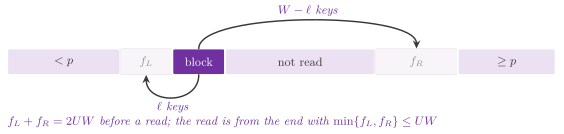
Lemma 12.26. In the partition of
vectorQuickSort(), no write overtakes a key not yet read.
Proof. Before a read, the free places at the two ends are \(f_L + f_R = 2 U W\), since each key read has been written and the \(2 U W\) keys loaded aside have not. Each read is from the end with \(\min\{ f_L , f_R \} \le U W\), and it frees \(U W\) places there. Hence, after it, both ends have at least \(U W\) free places, enough for the \(U W\) keys just read, however they split. \(\square\)
The pivot is the median of a sample of \(\max\{ 8 , W \}\) keys, one from each of as many equal stretches of the part at the same random offset, sorted by the network below. If the sample repeats the pivot, the partition keeps the minimum and the maximum of the part, and a second pass puts the keys equal to \(p\) apart. Past \(2 ( \lfloor \log_2 n \rfloor + 1 )\) levels a part is sorted by heapsort, as in the introsort of Musser 1997.
Lemma 12.27. vectorQuickSort() sorts \(n\)
keys in \(O( n \log n )\) time in the worst case.
Proof. Each level of the recursion partitions disjoint parts, in \(O( n )\) time in all with the choice of the pivots (a sample of a constant number of keys per part) and the second pass for the equal keys. Along each path the levels are at most \(2 ( \lfloor \log_2 n \rfloor + 1 )\), past which the heapsorts of the parts cost \(O( n \log n )\) in all (Theorem 12.7); the parts of at most \(16 W\) keys are sorted by a network of a constant size, and the counting is one pass. \(\square\)
A part of at most \(16 W\) keys is loaded into
\(M = 2^{\lceil \log_2 \lceil n / W \rceil \rceil}\) registers, the lanes past
\(n\) filled with the largest key, and sorted by a network of
compare-exchange steps, each a minimum and a maximum
(§12.12). With \(M \ge W\) the keys are held by
columns. The columns are sorted by the odd-even merge sort of Batcher
1968, register against register, and
then merged by a bitonic network whose comparators all go upwards; at last
each block of \(W\) registers is transposed. Here the steps within registers,
the dearer ones (a shuffle of the lanes besides the minimum and the maximum),
are then \(\frac{1}{2} \log_2 W ( \log_2 W - 1 )\) in all, besides a reversal
per merge and the transposition. Finally, two sorted runs are merged in the
registers (by the internal function vqs::mergeRuns()) as in the merge sort
of Chhugani et al.
2008. The register of the keys carried
over is merged by a bitonic merge with the next register of the run whose
next key is smaller, and the smaller \(W\) keys are written while the larger
are carried. In this way sort() merges the runs of the integers of 32 bits
(its internal mergeVectorRuns())
(§12.14).
12.8 Samplesort and the learned sort¶
Samplesort (Frazer and McKellar 1970)
generalizes the pivot to \(k - 1\) splitters drawn from a sample, which
distribute the items into \(k\) buckets in one pass; sampleSort() of
SampleSort.h is the super scalar samplesort of Sanders and Winkel
2004, in place as in the IPS\(^4\)o of
Axtmann et al. 2017 and Axtmann et
al. 2022 (Algorithm
12.16). It sorts by comparisons only, and therefore
takes any order; it is not stable.
In ADS/sort/SampleSort.h, the functions are declared as
// declarations of <ADS/sort/SampleSort.h>
template< class T , class C = std::less<> >
void sampleSort( std::vector< T > & A , C less = C() );
Algorithm 12.16. The in-place super scalar samplesort (Sanders and Winkel 2004; Axtmann et al. 2022).
Its sample has \(\alpha k - 1\) items, with
\(\alpha = \max\{ 1 , \lfloor ( \lfloor \log_2 n \rfloor + 1 ) / 5 \rfloor
\}\) (about \(0.2 \log_2 n\)), drawn at random (by a generator of fixed seed)
into the front of the part and sorted by pdqSort(), and every \(\alpha\)-th item of it is a
splitter. The \(k - 1\) splitters \(s_1 \le \cdots \le s_{k-1}\), \(k\) a power of
2, are laid out as a complete binary search tree in an array
\(t[ 1 .. k - 1 ]\), the children of \(t[ j ]\) in \(t[ 2 j ]\) and
\(t[ 2 j + 1 ]\), in the order of Eytzinger of
§9.3. An item \(x\) finds its bucket
\(i = | \{ h : s_h \le x \} |\) by \(\log_2 k\) steps
\(j \gets 2 j + [ t_j \le x ]\) from \(j = 1\), and \(i = j - k\) at the end
(Figure 12.6): an addition per step and no branch,
hence no comparison mispredicted. Also, four items go down the tree
together, one level of the four at a time, and their loads overlap.
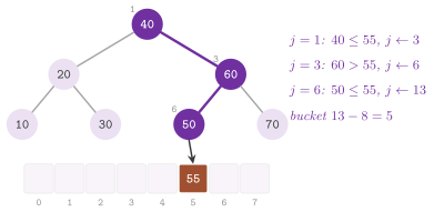
The number of buckets aims at buckets of 16 items after the last level: \(k = 2^\ell\) with \(\ell = \lfloor \log_2 ( n / 16 ) \rfloor\) (but at least 1) if it is at most 8, half of it (rounded up) if at most 16 (two levels then split alike), and 8 otherwise. If the sample has equal splitters, they are kept once and each bucket \(i > 0\) is split into the items equal to \(s_i\), which are done, and the others. In place, the distribution goes by blocks of \(b\) items (about 2 KiB) in three phases. First, the classification reads the items in order and puts each one into a buffer of \(b\) items of its bucket. A full buffer is written back to the front of the part as a block, which never overtakes the reading, since the items written and buffered are those read. Then the blocks are permuted into the areas of their buckets, each block going to the next place of its own bucket and swapping out the block there if it is not yet placed; each block thus moves once (twice through the two blocks of room). Finally, the cleanup gives each bucket, in the places of its range that no block covers, the items of its buffer and those of its last block that went past its end. A bucket of at most 64 items is then sorted at once, while it is in the cache, by an insertion sort.
Each item is read and written (roughly) twice per level, and with \(k = 256\)
there are about \(\lceil \log_{256} ( n / 16 ) \rceil\) levels. A bucket larger
than half the part, which only an unlucky sample gives, is sorted by
pdqSort().
Lemma 12.28. sampleSort() makes \(O( n
\log n )\) comparisons in the worst case, with \(O( k b )\) extra items for the
buffers. On distinct keys, with the sample drawn at random, it makes \(n
\log_2 n + O( n )\) comparisons in expectation.
Proof. A level classifies each item of a part with \(\log_2 k \le 8\)
comparisons, and the sample costs \(O( \alpha k \log ( \alpha k ) )\), i.e.,
\(O( m )\) for a part of \(m \ge 16 k\) items; the parts of a level are
disjoint, and hence a level costs \(O( n )\). A bucket that the recursion
enters holds at most half of its part, and thus the levels are at most
\(\log_2 n\); the buckets sorted by pdqSort(), disjoint as well, cost \(O( n
\log n )\) by Lemma 12.24. As for the expected count, it is the
analysis of Sanders and Winkel 2004,
for a sample of \(\alpha k - 1\) random items: each level compares an item
with \(\log_2 k\) splitters, and a bucket of more than \(( 1 + \varepsilon ) m
/ k\) items has a probability that falls exponentially in \(\alpha\) (cf.
(12.6) below). \(\square\)
The learned sort, learnedSort() of LearnedSort.h (after Kristo et al.
2020 and Ferragina and Odorisio
2025), keeps the splitters of
samplesort but replaces the search among them by a model of the cumulative
distribution function (CDF) \(F\) of the keys, \(F( x )\) the fraction of the
keys not larger than \(x\) (Algorithm 12.17). It
sorts the numbers of 32 or 64 bits in their natural order, the total order
of IEEE 754 for the floating point numbers, and gives bit for bit the
result of sort(). A distribution into \(k\) buckets is balanced when the
bucket of \(x\) is \(\lfloor k F( x ) \rfloor\), and the splitters at the
quantiles \(i / k\) of a sample approximate it within the error of the
empirical CDF \(F_s\) of the sample, which is bounded whatever \(F\) is.
Lemma 12.29. (Dvoretzky, Kiefer and Wolfowitz, with the constant of Massart) For a sample of \(s\) keys drawn independently from \(F\), and every \(\varepsilon > 0\),
Proof. The proof is in Massart 1990. \(\square\)
Lemma 12.30. Let the \(s\) keys of the sample be drawn independently and uniformly from the \(n\) keys of the input, and let the splitters be the quantiles \(i / k\) of the sample. Then, with probability at least \(1 - 2 e^{-2 s \varepsilon^2}\), each bucket holds at most \(( 1 / k + 2 \varepsilon ) n\) keys.
Proof. In effect, the sample is drawn from the empirical distribution \(F\) of the input, and (12.6) bounds by \(\varepsilon\) the distance of \(F_s\) from \(F\) everywhere, with the stated probability. Two consecutive splitters \(a < b\) have \(F_s( b^- ) - F_s( a ) \le 1 / k\), and hence \(F( b^- ) - F( a ) \le 1 / k + 2 \varepsilon\), which is the fraction of the keys in the bucket. \(\square\)
With \(s = 16 k\) and \(\varepsilon\) a small multiple of \(1 / \sqrt{s}\), each bucket thus holds \(n / k + O( n / \sqrt{k} )\) keys with high probability, as the sample of samplesort does. The model evaluates the number of splitters less than \(x\) by a grid of cells of equal width \(w\), a power of 2, on the range \([ S_{\min} , S_{\max} ]\) of the sample. Here the cell of \(x\) is \(\lfloor ( x - S_{\min} ) / w \rfloor\), a shift, and each cell keeps the number of splitters before it (a histogram of the sample and its prefix sums, i.e., a piecewise constant model of the CDF). If no cell holds more than \(c_{\max}\) splitters, the bucket of \(x\) is the count of its cell plus \(c_{\max}\) comparisons with no branch, in \(O( 1 )\) time instead of the \(\log_2 k\) dependent loads of a search, which is where the learned sorts gain on samplesort. In the papers, the models are linear splines and the recursive model index of the learned indexes of §6.4; the grid is the simplest model with the same guarantee.
In ADS/sort/LearnedSort.h, the functions are declared as
// declarations of <ADS/sort/LearnedSort.h>
template< VectorKey T >
void learnedSort( std::vector< T > & A );
Algorithm 12.17. The learned sort, \(b\) the size of a block and \(c_{\max}\) the most splitters in a cell.
The grid fails exactly where the keys are dense with respect to their mean
on the range (the laws with a heavy tail, such as those of Zipf and Pareto,
and the clusters far apart), where some cell of the finest grid allowed
holds more than \(c_{\max}\) splitters, or where the sample repeats its
quantiles (few distinct keys). Both are seen on the sample before any key
moves, and the sort then falls back to sampleSort(), whose buckets of
equal keys take care of the duplicates. A sample that repeats a splitter
only in part gives each repeated splitter a bucket of the keys equal to it,
which needs no sort (the buckets of equality of IPS\(^4\)o, as in the
LearnedSort 2.0 of Kristo et al. 2021).
detail::learnedSortIf() is the same sort that reports whether the model
fitted, returning false (and leaving the vector untouched) instead of
falling back. In §25.7, the parallel sorts use
it as the classifier of their distribution. When the model fits, the sample
and the model cost \(O( k \log k )\), the classification and the moves \(O( n
)\), and the sorts of the buckets by vectorQuickSort() \(O( n \log ( ( 1 / k + 2
\varepsilon ) n ) )\) on the event of Lemma 12.30, by
Lemma 12.27 on each bucket. Its extra room is a buffer of \(n\)
items and \(n\) bucket numbers of 16 bits. sort() does not choose it, since
on the measures of the benchmark of the library vectorQuickSort() sorted
the same inputs faster. It remains for the inputs where the model fits best
(keys of a smooth law, many buckets), on which it may well be faster, and as
the reference of the technique.
12.9 Heapsort and the sorts by trees¶
A max-heap on a vector has \(A[ \lfloor ( i - 1 ) / 2 \rfloor ] \ge A[ i ]\) for
each \(i > 0\), and hence its maximum in \(A[ 0 ]\). It is the binary heap of
§9.3, with the order reversed. Heapsort (Williams
1964; Montresor 2025,
§10.1.4; Morin 2013,
§11.1.3) builds such a heap in the vector
and then extracts its maximum \(n - 1\) times, each time into the place that the
heap frees at its end (Algorithm 12.18).
maxHeapRestore( A , i , dim ) of Heapsort.h moves the item of \(A[ i ]\)
down, swapping it with its larger child, when the subtrees of the children are
max-heaps in \(A[ 0 .. \mathit{dim} - 1 ]\). It is a loop, not the recursion of
the book (exercise 10.4 of Montresor
2025), so that the sort uses \(O( 1 )\)
extra space.
In ADS/sort/Heapsort.h, the functions are declared as
// declarations of <ADS/sort/Heapsort.h>
template< class T , class C = std::less<> >
void maxHeapRestore( std::vector< T > & A , std::size_t i , std::size_t dim ,
                     C less = C() );
template< class T , class C = std::less<> >
void heapBuild( std::vector< T > & A , C less = C() );
template< class T , class C = std::less<> >
void heapsort( std::vector< T > & A , C less = C() );
template< class T , class C = std::less<> >
bool isMaxHeap( const std::vector< T > & A , std::size_t dim , C less = C() );
Algorithm 12.18. The restoration of a max-heap, its construction from the bottom up, and heapsort (Montresor 2025, §10.1.4).
heapBuild() calls maxHeapRestore() from \(\lfloor n / 2 \rfloor - 1\) down
to 0, the places from \(\lfloor n / 2 \rfloor\) on being leaves, i.e., heaps
of one item: when the call on \(i\) comes, the subtrees of its children are
heaps already. This construction from the bottom up is that of Floyd
1964, and we now show that it is cheaper
than \(n\) insertions into a heap. isMaxHeap() checks the order of
a prefix of the vector, for the audits.
Lemma 12.31. heapBuild() takes \(O( n )\)
time and makes at most \(2 n + O( \log^2 n )\) comparisons in its walks down,
plus two per call.
Proof. A heap of \(n\) items has at most \(\lceil n / 2^{m+1} \rceil\) nodes of height \(m\), and the walk down from a node of height \(m\) goes down at most \(m\) levels, with two comparisons each. Hence the levels are at most
since \(\sum_{m \ge 1} m / 2^m = 2\) (the expected number of tosses of a fair coin up to the first head, as Morin 2013, §11.1.3 remarks). \(\square\)
Theorem 12.7. heapsort() sorts \(n\) items
in place in \(O( n \log n )\) time, with at most \(2 n \log_2 n + O( n )\)
comparisons.
Proof. After the construction, each of the \(n - 1\) extractions swaps the maximum with the last place of the heap, which shrinks by one, and walks down from the root of a heap of \(i < n\) items, at most \(\lfloor \log_2 i \rfloor\) levels with two comparisons each and two more at the last. With Lemma 12.31 the total is at most \(2 n \log_2 n + O( n )\). Finally, the places freed at the end receive the maxima in decreasing order, and the vector ends sorted. \(\square\)
Figure 12.7 shows the sort on the vector of exercise 11.1 of Morin 2013. In the book of Morin, the sort builds a heap of the minimum, extracts into the end of the vector, which leaves it in decreasing order, and reverses it at the end. A max-heap spares the reversal. In exercise 11.9 of its Java edition one should explain why the reversal is better not avoided by negating the comparator instead: a negation costs a little at each of the \(\Theta( n \log n )\) comparisons, while the reversal costs \(n / 2\) swaps once, and the max-heap avoids both. Furthermore, the bound of Theorem 12.7 is attained, as we show next.
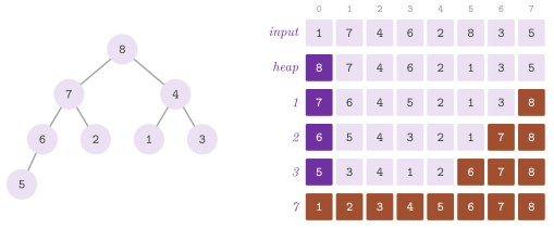
Lemma 12.32. For each \(n\) there is an
input of \(n\) distinct items on which heapsort() makes at least
\(2 n \log_2 n - O( n )\) comparisons, and likewise for the heapsort of
Morin 2013, with the order reversed
(exercise 11.8 there).
Proof. We build the input by running the sort backwards, as a max-heap
\(H_n\) that heapBuild() leaves as it is (no item is larger than its
parent), so that the sort replays the extractions chosen below. Let \(H_1\)
be one item, and let \(H_{i-1}\), a max-heap of \(i - 1\) items, be built.
Its least item \(x\) lies in a leaf \(p\), at the depth
\(k \ge \lfloor \log_2 ( i - 1 ) \rfloor - 1\), since the leaves of a heap
lie on its last two levels; let \(v_0 , \ldots , v_k = p\) be the path from
the root to \(p\). The heap \(H_i\) has a new item \(M\), larger than all the
others, at the root, the item of \(v_{j-1}\) in \(H_{i-1}\) at \(v_j\) for
\(1 \le j \le k\), the item \(x\) at the new last place \(i - 1\), and the items
of \(H_{i-1}\) elsewhere. It is a max-heap: along the path each item moved
down lies under one not smaller, the children of \(v_j\) off the path were
already below the item now at \(v_j\), and \(x\), the least item, is under
any parent. The extraction from \(H_i\) swaps \(M\) with \(x\), and then
maxHeapRestore() on \(i - 1\) items finds at each \(v_j\), \(j < k\), that the
larger child is \(v_{j+1}\), since its item was the parent in \(H_{i-1}\) of
the other child, and that it is larger than \(x\), a descendant of it in
\(H_{i-1}\); at \(p\), a leaf, it stops. Hence the extraction leaves
\(H_{i-1}\), and it makes at least \(2 k - 1\) comparisons (two at each \(v_j\),
\(j < k\), but at most one node with a single child). Summing over
\(i = 2 , \ldots , n\), with Lemma 12.3,
The heapsort of Morin, on a min-heap with the result reversed, is the same with the order of the items reversed. \(\square\)
On this input the sort phase walks almost to the bottom of the heap at
each extraction. The average over the inputs is of the same order:
Schaffer and Sedgewick 1993, who
analyse the heapsort of Williams with Floyd's construction, i.e., our
heapsort(), show that it moves about \(n \log_2 n\) keys on average and
about \(\frac{1}{2} n \log_2 n\) in the best case, hence (two comparisons
per level of a sift) about \(2 n \log_2 n\) comparisons on average; the
variant of Floyd that sinks the item to the bottom and then lifts it (the
bottom-up heapsort below) makes, by the same results, an asymptotically
optimal number of comparisons on average, about \(n \log_2 n\), and
\(\frac{3}{2}\) times as many in the worst case. The
inputs in order, increasing for the sort of Morin and decreasing for
heapsort(), are heaps already, and their sifts stop somewhat above the
bottom: we measured about \(0.66 \, n\) levels missed in all for \(n\) up to
\(2 \cdot 10^4\), which the count of the test below includes.
The test ods_ints.ods.ex11.8.heapsort-worst checks the count against
\(2 n \log_2 n - 4 n\) for both sorts, on \(n\) up to \(10^5\). The heap of
DaryHeap.h with the walk from the bottom up of Wegener
1993 saves about one comparison per
level on such inputs (§9.4).
Two more sorts of the area select by trees (Algorithm
12.19). The tree selection of Knuth 1998,
§5.2.3, tournamentSort() of
KnuthSorts.h, plays a knockout tournament on a complete binary tree \(W\)
whose \(L\) leaves are the items (padded with \(\bot\), which loses all its
matches). Its winner, i.e., the least item, goes out, its leaf becomes \(\bot\),
and only the matches on its path are played again. This is the idea from
which heapsort grew, and the tree of losers of
§9.11 refines it. The tree sort of exercise 6.1
of Montresor 2025, treeSort() of
TreeSort.h, inserts the items in a search tree of Chapter
8 and reads them back by the symmetric visit. Each key
keeps the number of its copies, and the repeated items are therefore not
lost. It runs on a Red-Black tree (the default, balanced) or on a
binary search tree with no balance, which makes it the example of the cost
of the balance.
Algorithm 12.19. The tournament sort (Knuth 1998, §5.2.3) and the tree sort (Montresor 2025, exercise 6.1).
In ADS/sort/TreeSort.h, the functions are declared as
// declarations of <ADS/sort/TreeSort.h>
template< std::totally_ordered T >
void treeSort( std::vector< T > & A , bool balanced = true );
Lemma 12.33. tournamentSort() makes at
most \(n - 1 + n \lceil \log_2 n \rceil\) comparisons, with \(O( n )\) extra
places, and it is stable. treeSort() takes \(O( n \log n )\) time in the
worst case on a Red-Black tree, and \(\Theta( n^2 )\) on a sorted input with
no balance.
Proof. Its tree has \(L < 2 n\) leaves, and its first round plays at most
\(n - 1\) matches with a comparison, those against \(\bot\) being free. Each
extraction plays again the \(\log_2 L = \lceil \log_2 n \rceil\) matches of
the path of the winner, and the tree and the output take \(2 L + n\) places.
A match between equal items goes to the left one, which came first in the
input, since the leaves are in the order of the places. As for treeSort(),
a Red-Black tree has height \(O( \log n )\) (§8.5.5), and
each of the \(n\) insertions follows one path; with no balance, the sorted
input makes the tree a path, and the \(i\)-th insertion walks \(i - 1\) nodes.
\(\square\)
12.10 The sorts by digits¶
The sorts of this section are not sorts by comparisons: they use the keys,
or parts of them, as indices into an array, and a statement such as
\(c[ a[ i ] ] \gets c[ a[ i ] ] + 1\) takes constant time but has as many
outcomes as the array has places; their execution is therefore not a binary
tree and Theorem 12.1 does not apply (Morin 2013,
§11.2). Counting Sort (countingSort() of
CountingSort.h, Montresor 2025, §2.7.5)
sorts integers in \([ 0 , k )\): \(B[ v ]\) counts the occurrences of \(v\), and
then each \(v\) is written \(B[ v ]\) times in order
(Algorithm 12.20), in \(\Theta( n + k )\) time and
\(\Theta( k )\) space, linear when \(k = O( n )\). Each key must be in
\([ 0 , k )\), a precondition checked key by key as the keys are counted.
Since it writes the keys back rather than the items, it suits only the keys
that are the whole item. Pigeonhole Sort (pigeonholeSort() of PigeonholeSort.h,
exercise 4.11 of the book) sorts instead the pairs
\(( \mathit{key} , \mathit{value} )\), appending each value to the List of
its key and reading the lists in the order of the keys; it thus takes \(O( n
+ k )\) time, \(n\) appends to the end of a list and a walk of the \(k\) lists,
and it is stable, since each list keeps the order of its appends.
In ADS/sort/CountingSort.h, the functions are declared as
// declarations of <ADS/sort/CountingSort.h>
template< class T >
void countingSort( std::vector< T > & A , std::size_t k );
Algorithm 12.20. Counting Sort and Pigeonhole Sort (Montresor 2025, §2.7.5 and exercise 4.11).
In ADS/sort/PigeonholeSort.h, the functions are declared as
// declarations of <ADS/sort/PigeonholeSort.h>
template< class V >
std::vector< std::pair< int , V > >
pigeonholeSort( const std::vector< std::pair< int , V > > & A , int k );
The counting sort of Morin 2013, §11.2.1, which carries the items along and is stable, is the pass of the radix sort below: the counts \(c\) are turned into their prefix sums \(c'\), i.e., \(c'[ v ]\) becomes the number of keys not larger than \(v\), and the items are scanned and each one is written into the next place of its key, which starts at \(c'[ v - 1 ]\) (or the scan goes backwards from the end, writing the item of key \(v\) into \(c'[ v ] - 1\) and decrementing \(c'[ v ]\), as in the book). Figure 12.8 shows it on the data of figure 11.7 of the book.
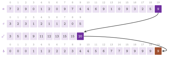
Theorem 12.8. The counting sort sorts \(n\) integers in \([ 0 , k )\) in \(O( n + k )\) time. Its version with the prefix sums is stable.
Proof. The counts and their prefix sums cost \(O( n )\) and \(O( k )\), the output \(O( n + k )\). In the version with the prefix sums, the items of key \(v\) fill the places \(c'[ v - 1 ] , \ldots , c'[ v ] - 1\) in the order of the scan; a forward scan from the starts, or a backward one from the ends, keeps among them the order of the input. \(\square\)
A radix sort applies a stable distribution to each digit of the keys, from the least significant to the most (LSD), as the machines for punched cards did one column at a time. Its correctness rests on the stability of each pass.
Lemma 12.34. If the keys have \(w / d\) digits of \(d\) bits, and each pass distributes the items stably by one digit, from the least significant to the most, then after the pass on the digit \(j\) the items are sorted by the number formed by their digits \(0 , \ldots , j\).
Proof. By induction on \(j\): after the pass on \(j\), two items with different digits \(j\) are in the order of those digits, and two with the same digit \(j\) keep the order that they had, i.e., by the inductive hypothesis, the order of their digits \(0 , \ldots , j - 1\). Equivalently (Morin 2013, §11.2.2), if \(x < y\) and their highest differing bit is \(r\), the pass on the digit \(\lfloor r / d \rfloor\) puts \(x\) before \(y\), and the later passes keep them so. \(\square\)
Theorem 12.9. For any \(d > 0\), the radix sort sorts \(n\) keys of \(w\) bits in \(O( ( w / d ) ( n + 2^d ) )\) time.
Proof. There are \(\lceil w / d \rceil\) passes, each a stable counting sort on \(2^d\) values, \(O( n + 2^d )\) by Theorem 12.8; Lemma 12.34 gives the correctness. \(\square\)
Corollary 12.1. Integers in \(\{ 0 , \ldots , n^c - 1 \}\) are sorted by the radix sort in \(O( c n )\) time.
Proof. With \(d = \lceil \log_2 n \rceil\), the keys have \(w \le c \lceil \log_2 n \rceil\) bits, hence at most \(c\) passes of \(O( n + 2^d ) = O( n )\) each. \(\square\)
Figure 12.9 shows the four passes on keys of 8 bits with digits of 2 bits, the data of figure 11.8 of Morin 2013.
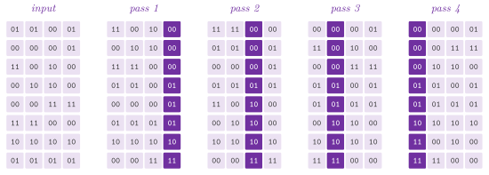
radixSort() of RadixSort.h is the LSD sort of the integers and of the
floating point numbers of at most 8 bytes (the concept RadixKey), with
bytes as digits, between the vector and a buffer
(Algorithm 12.21): \(O( w ( n + 256 ) )\) time for
keys of \(w\) bytes, and no comparison. Its keys come from radixKey(),
which makes the bits of a number an unsigned integer whose order is that of
the numbers: the sign bit flipped for a signed integer (exercise 11.13 of
Morin 2013, whose radix sort takes the
unsigned integers only), and for a floating point number all the bits
flipped if it is negative and the sign bit otherwise (Herf
2001). This key is the unsigned integer
of the width of the type, and it is declared as
// declarations of <ADS/sort/RadixSort.h>
template< RadixKey T >
void radixSort( std::vector< T > & A );
template< class T , class K >
void radixSortBy( std::vector< T > & A , K key );
template< RadixKey T >
void americanFlagSort( std::vector< T > & A );
void msdRadixSort( std::vector< std::string > & A );
template< RadixKey T >
auto radixKey( T x );
Lemma 12.35. For numbers of the same type, \(x < y\) implies \(\mathrm{radixKey}( x ) < \mathrm{radixKey}( y )\), with the order of IEEE 754 for the floating point numbers, \(-0\) before \(+0\) and the NaN at the two ends.
Proof. For the integers in two's complement, flipping the sign bit maps \([ -2^{w-1} , 2^{w-1} )\) onto \([ 0 , 2^w )\) by adding \(2^{w-1}\), which keeps the order. A floating point number of IEEE 754 is a sign bit followed by a magnitude whose order as an unsigned integer is that of the absolute values (Morin 2013, §11.3); setting the sign bit of the positive numbers puts them above all the negative ones, and complementing the negative ones reverses their order and clears their sign bit (a larger magnitude gives a smaller key). \(\square\)
Algorithm 12.21. The LSD radix sort of numbers by bytes.
A pass scatters the items from one array into the other by the prefix sums of the counts of its byte, as in the stable counting sort above: the count of each value of the byte becomes the place of the first item with that value, and each item, in order, goes to the place of its value, which then advances by one.
Three refinements make the passes fewer and cheaper. A first sweep finds
the bytes in which some keys differ, and only those make a pass; small keys
in wide types thus cost only the bytes they use. All their histograms
are counted in a second sweep (Herf 2001).
When the keys differ in one byte only, the byte determines the number, and a
counting sort writes the numbers back from one of each value, with no
buffer. A vector larger than the cache (1 MiB) whose keys differ in three
bytes or more first goes by its top byte into the buffer, the one pass that
scatters over the whole memory. Each part is then sorted by the other bytes
while it fits in the cache (an MSD pass before the LSD ones), which is still
correct by Lemma 12.34, since the parts are the
items with the same top byte, in the order of that byte. On any items, the same sort, by an unsigned key that a function gives, is radixSortBy(),
which is stable too, e.g., for records sorted by one field.
The radix sorts from the most significant digit (MSD) distribute by the
first digit and recur on each bucket, reading only the digits that tell the
keys apart. The American flag sort of McIlroy et al.
1993, americanFlagSort(), does it in
place (Algorithm 12.22). Two scans that stop at the
first pair out of order find a vector already sorted or in reverse order
(which is reversed), and a sweep finds the bytes in which some keys differ. The items
are then permuted into the 256 buckets of the first byte that differs, as
the flag of the name is divided into stripes, and each bucket is sorted in
the same way by the next byte. The permutation does not follow its cycles,
whose every step waits for the load of the step before: each item of the
part of a bucket not yet in place is swapped to the next free place of its
own bucket, and the buckets are taken in turn until all are full; the loads
of a round are then independent (Skarupke
2016); Figure
12.10 shows the rounds on twelve keys. A bucket of
fewer than kFlagSmall items (8192 when the vector registers are there,
256 otherwise) is left to vectorQuickSort(), whose order on the floating
point numbers is the one of the keys, or, without the registers, to
pdqSort(). It is not stable.
Lemma 12.36. americanFlagSort() sorts \(n\)
keys of \(w\) bytes in \(O( w n )\) time, with \(O( 1 )\) extra space per level of
the recursion besides the 256 counts, and no buffer of the items.
Proof. A part of \(m\) items costs \(O( m + 256 )\) for its counts and its permutation, each round of which puts at least one item in its place. A part enters the recursion only if it has at least \(\mathtt{kFlagSmall} \ge 256\) items, and hence the parts of a level are at most \(n / 256\), and the 256 of each cost \(O( n )\) in all; the levels are at most \(w\), one per byte. Finally, the buckets of fewer than \(\mathtt{kFlagSmall}\) items, a constant, are sorted in \(O( 1 )\) time per item. \(\square\)
Algorithm 12.22. The American flag sort, \(b_d( x )\) the byte \(d\) of the key of \(x\) and \(D\) the bytes in which some keys differ.
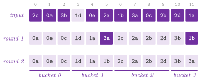
Two older sorts by digits of Knuth 1998
are in KnuthSorts.h (Algorithm 12.23).
The address calculation sort of Isaac and Singleton
1956, addressCalculationSort(), inserts
each number into one of \(M\) sorted lists by its value, the list \(i\) taking
the numbers in the \(i\)-th of \(M\) equal ranges between the least and the
largest, as one files cards under the letters (\(M = \lfloor n / 4 \rfloor +
1\) by default). The radix exchange of Hildebrandt and Isbitz
1959 (Algorithm 5.2.2R of Knuth),
radixExchangeSort(), is the quicksort on the bits of the keys from the
most significant: each part is split into the keys with the bit 0 and those
with the bit 1, by exchanges as in a partition, and each half is sorted on
the next bit.
Algorithm 12.23. The address calculation sort (Isaac and Singleton 1956) and the radix exchange sort (Knuth 1998, §5.2.2).
Lemma 12.37. addressCalculationSort() is
stable, takes \(\Theta( n^2 )\) time in the worst case, and \(O( n )\) expected
time on \(n\) numbers drawn independently and uniformly from an interval.
radixExchangeSort() sorts \(n\) keys of \(w\) bits in \(O( n w )\) time, and it
is not stable.
Proof. A number goes to the end of its list and moves back past the larger ones only, and hence the equal numbers keep their order; the lists are read in the order of their ranges. If all the numbers but one fall in the same list, e.g., with one far larger than the others, the insertions into it cost \(\Theta( n^2 )\). With uniform numbers, the size \(N_i\) of the list \(i\), besides the least and the largest number, which set the range, is binomial with at most \(n\) trials and mean at most \(n / M < 4\); the insertions into it cost \(O( 1 + N_i^2 )\), whose expectation is less than \(1 + 4 + 16\), and the \(M\) lists cost \(O( n )\) in expectation. As for the radix exchange, each level of the recursion, one per bit, scans its disjoint parts once. On \(2 , 2' , 1\) (in binary \(10\), \(10\), \(01\)) the split on the first bit exchanges \(2\) and \(1\), and the output is \(1 , 2' , 2\). \(\square\)
12.11 Sorting strings¶
A comparison of two strings costs as much as their common prefix, and a sort of strings by comparisons may thus read the same characters "many" times. The sorts of this section read instead each character of the distinguishing prefixes (the shortest prefix of each string that is not a prefix of another one, of total length \(D\)) a bounded number of times, and \(D\) characters must be read by any sort of distinct strings.
Lemma 12.38. A sort of \(n\) distinct strings that reads their characters reads all the \(D\) characters of their distinguishing prefixes on some input.
Proof. Let the character \(i\) of the string \(s\) lie in its distinguishing
prefix, of length \(j \ge i\); then some other string \(t\) has the first \(j - 1\)
characters of \(s\), which therefore include the character \(i\) unless \(i = j\),
where \(t\) has a different character or ends. If the sort never read that
character of \(s\), changing it to a character above or below that of \(t\) at
the same place, and above or below the character \(j\) of \(t\), would leave its
reads unchanged and its output the same, while the order of \(s\) and \(t\)
changes for one of the two choices. \(\square\)
msdRadixSort() of
RadixSort.h sorts strings by their characters from the first, the end of
a string before every character (Algorithm 12.24).
Its first pass permutes the strings into their buckets in place, as the
American flag sort does. Then each bucket has a buffer, made only if some
bucket is not all of equal strings, between which and the vector the
strings go back and forth, one move per pass, the character of each string
read once per pass and kept aside. The prefix that all the strings of a
group share is first skipped by comparing them with one of them; hence a
group of equal strings, or of strings with a long common prefix, costs one
comparison instead of one pass per character, and the groups of at most 16
strings are sorted by insertion (McIlroy et al.
1993; Kärkkäinen and Rantala
2008).
Lemma 12.39. msdRadixSort() sorts \(n\)
strings in \(O( ( 1 + \sigma / 16 ) D + n )\) time.
Proof. A pass on a group of \(m > 16\) strings costs \(O( m + \sigma )\), and the character it reads of each string, as the common prefix it skips, lies in its distinguishing prefix, since the other strings of the group share the characters before it; the passes are thus at most \(D / 17\), and they cost \(O( D + \sigma D / 16 )\) in all. A group of at most 16 strings is sorted by insertion with fewer than \(16^2\) comparisons, each of which reads the common prefix of two strings and one character more, within their distinguishing prefixes; these cost \(O( D + n )\). \(\square\)
Algorithm 12.24. The MSD radix sort of strings, \(c_d\) the character \(d\) of a string, \(c_d = 0\) past its end.
The multikey quicksort of Bentley and Sedgewick
1997, multikeyQuickSort() of
MultikeyQuickSort.h as chapter 7 of Ferragina
2023 presents it, is the quicksort of
strings by one character at a time (Algorithm
12.25): a partition into three parts, the strings
whose character \(d\) is smaller, equal and larger than that of the pivot,
the equal part going on with the character \(d + 1\) and the others with \(d\).
It is the sort that corresponds to the ternary search tree of the same
paper, and its pivot is the first string of the part. It sorts in place and
is not stable.
Lemma 12.40. multikeyQuickSort() makes at
most \(( \sigma + 2 ) ( D + n )\) comparisons of characters on \(n\) strings
over an alphabet of \(\sigma\) characters; on a random order of distinct
strings it makes \(O( D + n \log n )\) in expectation.
Proof. A comparison of the character \(d\) of a string with the pivot sends the string either to the equal part, which goes on with \(d + 1\), or to the smaller or the larger part, whose characters at \(d\) are fewer than before by the one of the pivot. This first case happens at most once per character of the distinguishing prefix of the string and once more at its end, i.e., \(D + n\) times in all, since a string alone in its part is done; the second happens at most \(\sigma + 1\) times per string and value of \(d\), the end of a string counting as a character. On a random order the pivot of each part is a random string of it, and the bound is that of Bentley and Sedgewick 1997. \(\square\)
The bound in expectation is against the \(O( n \log n )\) comparisons of whole strings of a quicksort, each as long as a common prefix (which may be "long").
In ADS/sort/MultikeyQuickSort.h, the functions are declared as
// declarations of <ADS/sort/MultikeyQuickSort.h>
void multikeyQuickSort( std::vector< std::string > & A );
Algorithm 12.25. The multikey quicksort (Bentley and Sedgewick 1997), \(v < 0\) for the end of a string.
prefixKeySort() of StringSort.h reads each string a few times in all
and leaves the work to the quicksort of integers in the vector registers
(Algorithm 12.26). A group of strings that agree on
their first \(d\) characters is sorted in one step: the longest prefix that
they share from \(d\) is skipped. Each string \(i\) gets the integer key \(k_i =
\lfloor w_i / 2^b \rfloor 2^b + i\), where \(b = \lceil \log_2 | G | \rceil\)
and \(w_i\) is the number of 64 bits whose bytes, from the most significant,
are the characters \(d , \ldots , d + 7\) of the string (0 past its end). The
order of the keys is thus that of the strings on those \(64 - b\) bits and
then that of their places, which makes the sort stable. Next, the keys are
sorted by vectorQuickSort(), the strings
moved once to their places, and the runs of equal
\(\lfloor k_i / 2^b \rfloor\), which agree on the characters up to
\(d + \lfloor ( 64 - b ) / 8 \rfloor\), are sorted in turn from there. A step
that leaves a group of more than \(3 / 4\) of its strings counts against a
budget of \(2 \log_2 n\) such steps, past which a group goes to
std::stable_sort() on the characters from \(d\). So does a group that a step
does not split (strings holding the character 0, which the padding shares).
Its extra room is \(n\) keys of 64 bits and \(n\) strings.
Lemma 12.41. The steps of prefixKeySort()
are nested at most \(\log_{4/3} n + 2 \log_2 n\) deep, and they take \(O( D + n
\log^2 n )\) time, besides the sorts of the groups left to
std::stable_sort().
Proof. A step either leaves each of its groups with at most \(3 / 4\) of its strings, or uses one of the \(2 \log_2 n\) steps of the budget, which gives the depth. A step on a group of \(m\) strings reads at most 8 characters of each beyond the common prefix it skips, which lies in the distinguishing prefixes of all of them, and it sorts the \(m\) keys in \(O( m \log m )\) time (Lemma 12.27); the groups of one depth are disjoint, and hence a depth costs \(O( n \log n )\) beyond the characters of the distinguishing prefixes. \(\square\) In their string samplesort, Bingmann and Sanders 2013 use keys of prefixes in a similar way.
In ADS/sort/StringSort.h, the functions are declared as
Algorithm 12.26. The sort of strings by integer keys of their prefixes, \(w_i\) the 8 characters of the string \(i\) from \(d\) as a number of 64 bits.
Finally, the suffixes of one string are sorted by the algorithms of §15.5, which use that they share their characters.
12.12 Sorting networks¶
A sorting network is a fixed sequence of comparators \(( i , j )\),
\(i \ne j\), each of which puts the smaller of \(A[ i ]\) and \(A[ j ]\) in
\(A[ i ]\) and the larger in \(A[ j ]\), whatever the input. The comparators of
a round touch disjoint places and may run in parallel, in hardware, in the
lanes of a vector register or on a GPU. SortingNetworks.h represents a
comparator as a Comparator, the pair of its places, and a network as a
vector of them, which applyNetwork() runs on a vector
(Algorithm 12.27). Whether a network sorts all its
inputs is decided by the inputs of zeros and ones only, as we now show.
Lemma 12.42. (The 0-1 principle) A network of comparators sorts every input of \(n\) items if and only if it sorts the \(2^n\) inputs of zeros and ones.
Proof. A comparator commutes with every non-decreasing function \(f\) of the items, since \(\min\{ f( a ) , f( b ) \} = f( \min\{ a , b \} )\) and likewise for the maximum. Hence the network maps \(f( A )\) to \(f\) of its output on \(A\). If the output on some \(A\) has \(y_i > y_{i+1}\), the threshold \(f( z ) = [ z \ge y_i ]\) gives an input of zeros and ones whose output has a 1 before a 0. \(\square\)
The merge exchange of Batcher (Algorithm M of Knuth 1998,
§5.2.2) for any \(n\) is
mergeExchangeNetwork(), and the bitonic sorter of Batcher
1968 for \(n\) a power of 2 is
bitonicNetwork(). Both have \(O( n \log^2 n )\) comparators in \(O( \log^2 n
)\) rounds (Lemma 12.44 below), more than the \(O( n
\log n )\) comparisons of Theorem 12.1, which they pay
for with their parallelism. A sequence is bitonic if it first
increases and then decreases, or is a rotation of such a sequence. Two
halves sorted in opposite directions form one, and the bitonic sorter of
\(k\) items sorts its two halves in opposite directions and then applies the
half-cleaners of \(k , k / 2 , \ldots , 2\) items, a half-cleaner comparing
each item of the first half with the item \(k / 2\) places after it
(Figure 12.11).
Lemma 12.43. A half-cleaner applied to a bitonic sequence of zeros and ones gives two bitonic halves, no item of the first larger than an item of the second, one of the two halves being all zeros or all ones.
Proof. A sequence of zeros and ones is bitonic if and only if its ones, read cyclically on the places \(0 , \ldots , k - 1\), form one block of consecutive places (possibly empty or wrapping around the end), and likewise its zeros. Let the block of the ones have \(b\) places. If \(b \le k / 2\), no pair \(( i , i + k / 2 )\) of the half-cleaner holds two ones, since the block would then span more than \(k / 2\) places; hence every minimum is 0, and the maxima carry the ones of the block, the one at the place \(p\) going to the place \(p \bmod ( k / 2 )\) of the second half. The block, of at most \(k / 2\) consecutive places taken modulo \(k\), falls modulo \(k / 2\) onto as many consecutive places of the half taken cyclically, with no two of them on the same place; hence the maxima are bitonic, and so are the minima, all zeros. If \(b > k / 2\), the block of the zeros has fewer than \(k / 2\) places, and the same argument with the roles of zeros and ones exchanged makes every maximum 1 and the minima bitonic. In both cases one half is constant, the minima are 0 or the maxima are 1, and no item of the first half exceeds one of the second. \(\square\)
The comparators of bitonicNetwork() point the other way in the blocks
that must come out decreasing, which is the test \(i \mathbin{\&} k \ne 0\)
of its pseudocode.
Lemma 12.44. For \(n = 2^t\),
bitonicNetwork( n ) sorts any input of \(n\) items, with \(t ( t + 1 ) / 2\)
rounds of \(n / 2\) comparators each. mergeExchangeNetwork( n ) sorts any
input of \(n\) items with \(O( n \log^2 n )\) comparators in \(\lceil \log_2 n
\rceil ( \lceil \log_2 n \rceil + 1 ) / 2\) rounds.
Proof. By the 0-1 principle (Lemma 12.42) it suffices to sort the inputs of zeros and ones. By induction on \(k\), the half-cleaners of \(k , k / 2 , \ldots , 2\) items sort a bitonic sequence of \(k\) zeros and ones: the first leaves two bitonic halves with no item of the first above one of the second (Lemma 12.43), which the others sort independently. In turn, the sorter of \(k\) items sorts its two halves in opposite directions, by induction, which makes a bitonic sequence, and it then applies those half-cleaners. As for the rounds, the merges of the blocks of \(2^j\) items, for \(j = 1 , \ldots , t\), take \(j\) rounds each, \(t ( t + 1 ) / 2\) in all, and each round compares the \(n\) places in pairs. Finally, the merge exchange is Algorithm M of Knuth 1998, §5.2.2, where its correctness, its rounds and its comparators are proved. \(\square\)
In ADS/sort/SortingNetworks.h, the functions are declared as
// declarations of <ADS/sort/SortingNetworks.h>
std::vector< Comparator > mergeExchangeNetwork( std::size_t n );
std::vector< Comparator > bitonicNetwork( std::size_t n );
template< class T , class C = std::less<> >
void applyNetwork( std::vector< T > & A , const std::vector< Comparator > & N ,
                   C less = C() );
Algorithm 12.27. The application of a network, the bitonic sorter and the merge exchange (Batcher 1968; Knuth 1998, §5.2.2), \(\oplus\) and \(\&\) the exclusive or and the and of the bits, \(t = \lceil \log_2 n \rceil\).
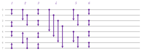
The networks of the vector quicksort (§12.7) sort up to \(16 W\) keys in the registers in this way, a comparator being a minimum and a maximum of two registers.
12.13 Sorting a file larger than the memory¶
A file larger than the memory is sorted in two phases, which
ExternalSort.h realizes as Knuth 1998, §5.4.1 and
§5.4.2 describes them for tapes, here on
sequences in memory that play the files (Algorithm
12.28). We describe the sorts on the blocks of an
external memory in Chapter 23. The first phase,
replacementSelection(), makes the initial runs with a heap of \(M\) items:
the least item of the current run goes out, and the next input item takes
its place, in the current run if it is not smaller than the item just
written and in the next run otherwise (the heap orders the pairs of a run
number and an item). Table 12.5 follows it with
\(M = 3\).
Table 12.5. replacementSelection() with
\(M = 3\) on \(5 , 8 , 3 , 9 , 1 , 7 , 2 , 6 , 4\): the item written, its run,
and the heap after the next input item has entered it (as pairs of a run
and an item); the runs are \(3 , 5 , 8 , 9\) and \(1 , 2 , 4 , 6 , 7\), longer
than \(M\).
| Out | Run | Heap after it |
|---|---|---|
| 3 | 0 | \(( 0 , 5 )\), \(( 0 , 8 )\), \(( 0 , 9 )\) |
| 5 | 0 | \(( 0 , 8 )\), \(( 0 , 9 )\), \(( 1 , 1 )\) |
| 8 | 0 | \(( 0 , 9 )\), \(( 1 , 1 )\), \(( 1 , 7 )\) |
| 9 | 0 | \(( 1 , 1 )\), \(( 1 , 2 )\), \(( 1 , 7 )\) |
| 1 | 1 | \(( 1 , 2 )\), \(( 1 , 6 )\), \(( 1 , 7 )\) |
| 2 | 1 | \(( 1 , 4 )\), \(( 1 , 6 )\), \(( 1 , 7 )\) |
| 4, 6, 7 | 1 | the heap empties |
Lemma 12.45. Every run of
replacementSelection() but the last has at least \(M\) items, a sorted
input gives a single run, and on a random input the runs have about \(2 M\)
items on average.
Proof. When a run starts, the heap holds \(M\) items, all of the new run, and each of them is written into it. An item enters the current run only if it is not smaller than the last written, which keeps the run sorted, and on a sorted input each item does. The average \(2 M\) is the snowplow argument of Knuth 1998, §5.4.1: in the steady state, the items of the next run accumulate in the heap at the rate at which the plow removes those of the current one. \(\square\)
The second phase, polyphaseMerge() (Algorithm 5.4.2D of Knuth, after
Gilstad 1960), merges the runs on \(T\)
tapes, \(T - 1\) of input and one of output. The runs are dealt so that their
counts on the tapes are a perfect Fibonacci distribution of order \(T - 1\),
padded with empty (dummy) runs: the distribution of a level,
\(a_1 \ge \cdots \ge a_{T-1}\), gives that of the next one as
\(a'_i = a_1 + a_{i+1}\), with \(a_T = 0\). Each phase merges runs from all the
input tapes onto the output one until one input tape is empty, which becomes
the next output. With three tapes and 13 runs, for instance, the counts go
\(( 8 , 5 , 0 ) \to ( 3 , 0 , 5 ) \to ( 0 , 3 , 2 ) \to ( 2 , 1 , 0 ) \to
( 1 , 0 , 1 ) \to ( 0 , 1 , 0 )\). Each item takes part in about
\(\log_\phi r\) merges for \(r\) runs with three tapes, \(\phi\) the golden ratio,
fewer with more tapes (Knuth 1998, §5.4.2), and no tape is ever only copied, which is, in fact,
the advantage of the polyphase merge over the balanced one. externalSort() is
the two phases together, and the function can report the phases it made.
In ADS/sort/ExternalSort.h, the functions are declared as
// declarations of <ADS/sort/ExternalSort.h>
template< class T , class C = std::less<> >
std::vector< std::vector< T > >
replacementSelection( const std::vector< T > & input , std::size_t M ,
                      C less = C() );
template< class T , class C = std::less<> >
std::vector< T > polyphaseMerge( std::vector< std::vector< T > > runs ,
                                 std::size_t tapes , C less = C() ,
                                 std::size_t * phases = nullptr );
template< class T , class C = std::less<> >
std::vector< T > externalSort( const std::vector< T > & input , std::size_t M ,
                               std::size_t tapes , C less = C() );
Algorithm 12.28. The replacement selection, the polyphase merge and the external sort (Knuth 1998, §5.4.1 and §5.4.2).
The merge of \(k\) runs at once, fed by one block per run, is the step of the multiway mergesort. Its trees of losers and its funnels are in §9.11.
12.14 The sort that chooses¶
sort() and stableSort() of Sort.h look at what they sort and pick,
among the sorts of the chapter, the one that suits it
(Algorithm 12.29). The thresholds between the
algorithms, kRadix (512) items for the numbers and the other items copied
as bytes, kStrings (64) for the strings and kRuns (16) runs, are
constants of the namespace, measured by the benchmark of the library
against std::sort, std::stable_sort and the sorts of Boost, and a
program may read them.
Algorithm 12.29. The choices of sort()
and of stableSort(), \(r\) the number of runs.
Its choices follow the type of the items and the order. With the natural
order on integers or floating point numbers of 32 or 64 bits and the sort
of Highway there (kVectorSort), a short vector goes to vectorQuickSort().
A long one with at most kRuns runs, counted by a pass that stops at the
run \(\mathtt{kRuns} + 1\) and keeps where they end, has its runs merged with
no second search for them (those of integers of 32 bits two by two in the
registers of the portable code, the others by the merges of powerSort(),
\(O( n \log r )\) for \(r\) runs). One of integers of 64 bits whose sample of 64
keys differs in one byte goes to the counting of radixSort(), and any
other to vectorQuickSort(). With the natural order on the other numbers,
or with no vector registers, a short vector goes to pdqSort() and a long
one in few runs to the merges. A sample of 64 keys that shows at most 16
distinct keys differing in 4 bytes or more sends it to pdqSort(), whose
three-way partitions sort \(k\) keys in \(O( n \log k )\) with fewer passes,
and the rest goes to radixSort(). With the natural order on strings, few
runs go to the merges, and the others to prefixKeySort() when the vector
registers are there (unless a sample shows at most 16 distinct strings) and
to msdRadixSort() otherwise. With any other order, items copied as bytes
go to pdqSort() below kRadix items, to the merges if they have few runs,
and otherwise to sampleSort(). Any other item goes to pdqSort() or, from
kRadix items, to sampleSort().
stableSort() makes the same choices where two equal items cannot be told
apart (the numbers and the strings), but for the floating point numbers that
hold a \(-0\), which std::less finds equal to \(+0\): these go to
powerSort() below kRadix items and to radixSortBy() with \(-0\) and
\(+0\) as one key from there. For the items copied as bytes it merges few
runs, and it counts by their keys the vectors whose sample of 64 shows at
most 16 distinct keys that all the items have (each item found among the
keys by a binary search with no branch, through a buffer of \(n / 2\) items).
It sorts the others by a merge sort through a buffer of \(n / 2\) items, as
the spinsort of Boost does (Tapia 2018):
the halves are sorted with the other array as their room and merged back
with no branch on the order, from both ends at once. Any other item goes to
powerSort().
Hence, pdqSort() and powerSort() are, besides the algorithms of their
sections, the engines of sort() and of stableSort() on the items that
none of the faster routes takes, and the two functions keep them also where
Boost is found. On our benchmark boost::sort::pdqsort and
boost::sort::spinsort are usually no slower, and faster on reversed keys
(which the check for one run below takes first, when the items are copied
as bytes) and on few distinct keys, respectively. A program that wants them
may call them directly on the vector; we have not changed the engines
inside the dispatch, since the change should first be measured on an idle
machine.
Two fast paths come before the choices. A vector of \(2^{14}\) items or more
(detail::kOneRun) copied as bytes, of any type and order, is first checked
for one run. If it is strictly decreasing, it is reversed in the same pass
that checks it, 32 pairs of items from the two ends at a time, checked
before they are swapped (and swapped back if a later block is out of order). Otherwise it is
scanned for an item smaller than the one before it, 64 items at a time,
with a prefetch by software ahead of the scan on the processors where the
hardware prefetcher falls behind. Hence a sorted or reversed vector costs
one pass.
Lemma 12.46. On numbers, sort() takes \(O( n
\log n )\) time in the worst case, and a vector of at least \(2^{14}\) items
copied as bytes that is sorted or strictly decreasing costs it one pass.
Proof. On numbers, the sorts it chooses take \(O( n \log n )\) time in the
worst case: vectorQuickSort() by Lemma 12.27,
pdqSort() by Lemma 12.24, radixSort() with its
counting by Theorem 12.9, with \(w \le 8\) bytes, and
the merges of at most \(\mathtt{kRuns}\) runs in \(O( n \log \mathtt{kRuns} )\)
by Theorem 12.4, since \(H \le \log_2 r\); the passes
that count the runs and sample the keys cost \(O( n )\). Its fast path reads
each item once, and it either reverses the vector in the same pass or finds
the first item smaller than the one before it. \(\square\) A NaN breaks the natural order, and a vector with a NaN has
therefore no defined order under std::less (the sorts by keys put it at an end).
12.15 Discussion and references¶
Sorting is the most studied problem of the field, and Knuth 1998 remains its reference: there one finds the merge sort, attributed to von Neumann (1945), the elementary sorts and their variants, Shell Sort and its gaps, the tree selection, the networks of Batcher and the 0-1 principle, the merge insertion of Ford and Johnson 1959, the replacement selection and the polyphase merge. Quicksort is due to Hoare 1962, and its classical analysis and engineering to Sedgewick 1978 and Bentley and McIlroy 1993, from whom the partition in three and the ninther in sorts of libraries come. Heapsort is due to Williams 1964, and the construction of the heap from the bottom up in \(O( n )\) to Floyd 1964. As for the lower bound of the sorts by comparisons, it appears to be folklore. The counting and the radix sorts go back to Seward (1954), and the radix sort to the machines that sorted punched cards one column at a time, as Morin 2013, §11.3 recalls; that chapter of Morin is the model of §12.2 to §12.10, with its exercises. Our textbook sorts are those of Montresor 2025 and of Ferragina 2023, whose chapters 5 and 7 present the quicksorts in three and with two pivots and the multikey quicksort.
The engineered quicksorts of the area follow the literature of the last
decades, from the introsort of Musser
1997 to the pattern-defeating quicksort
of Peters 2021, the partition by blocks
of Edelkamp and Weiß 2016 and the
analysis of the dual-pivot quicksort by Wild and Nebel
2012. The super scalar samplesort is that
of Sanders and Winkel 2004, in the
in-place form of Axtmann et al. 2022;
the vectorized quicksorts follow Bramas
2017, Gueron and Krasnov
2016 and Wassenberg et al.
2022, and the merges in the registers
Chhugani et al. 2008. The learned sort
follows the ideas of Kristo et al. 2020,
Kristo et al. 2021, Ferragina and
Odorisio 2025, Carvalho
2022 and Sato and Matsui
2024. The radix sorts follow McIlroy et
al.
1993 and Kärkkäinen and Rantala
2008, and the adaptive merge sorts follow
McIlroy 1993, Peters
2002 and Munro and Wild
2018, while the bounds of Timsort are
those of Auger et al. 2018. The adversary of
McIlroy 1999 shows that no quicksort
with a pivot taken among few items is safe from a comparator that answers
adaptively, which is one more reason for the fallbacks to heapsort. It is
fair to remark that the comparisons of the sorts in time, which decide the
thresholds of sort(), depend on the machine. They are left to the
appendix of the benchmarks, measured on an idle machine.
The sorts that the parallel executors run, by merging and by distribution, are in §25.7, the selection of the \(k\)-th item in §6.8, and the merge of \(k\) sorted sequences, the sequence heap and the heaps on which heapsort rests in Chapter 9.
12.16 Exercises¶
Each exercise names the test of the library that solves it (run it with
ctest -R <name>). We list first the exercises of chapter 11 of Morin
2013, in their order.
- Illustrate the execution of merge sort and of heapsort on
\(1 , 7 , 4 , 6 , 2 , 8 , 3 , 5\), and give one possible execution of
quicksort on the same vector (Morin 2013, exercise
11.1; our
Figure 12.4, Figure 12.7
and Table 12.4). Test:
ods_ints.ods11.1.sorts. - Sort a doubly linked list by merge sort with no auxiliary array, by
relinking its cells, and check that each item keeps its cell and that
the sort is stable (Morin 2013, exercise
11.2). Test:
ods_ints.ods.ex11.2.list-merge-sort. - Give an input of length \(n\) on which a quicksort with the first item as
the pivot makes \(\binom{n}{2}\) comparisons, one for the middle item as
the pivot, one for any rule that does not look at the values, and a
comparator that forces \(\binom{n}{2}\) comparisons out of a quicksort
(Morin 2013, exercises 11.3 to 11.6;
Lemma 12.23). Test:
ods_ints.ods.ex11.6.quicksort-adversary. - Compute the expected comparisons of the quicksort of Morin's book
exactly, and show that \(2 n H_n - n + H_n\) is not their expectation
(Morin 2013, exercise 11.7;
Lemma 12.20). Test:
ods_ints.ods.ex11.7.quicksort-expectation. - Describe an input on which heapsort makes at least
\(2 n \log_2 n - O( n )\) comparisons, and explain why the reversal at the
end of the heapsort of the book should not be replaced by a negated
comparator (Morin 2013, exercise
11.8, and exercise 11.9 of its Java
edition;
Lemma 12.32). Test:
ods_ints.ods.ex11.8.heapsort-worst. - Find another pair of permutations of \(1 , 2 , 3\) that the comparison
tree of Figure 12.2 does not both sort, and prove
that \(\log_2 n! = n \log_2 n - O( n )\), that a binary tree with \(k\)
leaves has height at least \(\log_2 k\), and that a random leaf of it has
expected depth at least \(\log_2 k\) (Morin 2013, exercises 11.9 to
11.12;
Lemma 12.1 to
Lemma 12.3). Test:
ods_ints.ods.ex11.9.comparison-tree. - Write a radix sort that sorts signed integers correctly, with the
extremes of each width (Morin 2013, exercise
11.13;
Lemma 12.35). Test:
ods_ints.ods.ex11.13.signed-radix-sort. - Sort by Selection Sort and by Insertion Sort, counting the comparisons
and the moves of each against Lemma 12.6
(Montresor 2025, §2.7.1 and §2.7.2).
Tests:
ch02.sec2.7.1.selection,ch02.sec2.7.2.insertion. - Sort by Merge Sort, recursively and from the bottom up, and sort a list
by Merge Sort and by Quicksort through the operations of the SEQUENCE
(Montresor 2025, §2.7.3 and exercises 12.1 and
12.5). Tests:
ch02.sec2.7.3.merge-sort,ch12.ex12.5,ch12.ex12.1. - Check the lower bound of the sorts by comparisons on the comparison
tree of the book (Montresor 2025, §2.7.4).
Tests:
ch02.sec2.7.4.lower-bound,pearls_io.ch5.lower-bounds. - Sort integers in \([ 0 , k )\) by Counting Sort, and pairs by Pigeonhole
Sort, stably (Montresor 2025, §2.7.5 and exercise
4.11). Tests:
ch02.sec2.7.5.counting-sort,ch04.ex4.11,contract_sort.counting-pigeonhole. - Build a max-heap from the bottom up, sort by heapsort, and restore the
heap by a loop instead of the recursion (Montresor 2025, §10.1.4 and
exercises 10.2 and 10.4). Tests:
ch10.sec10.1.4.heapsort,ch10.ex10.2,ch10.ex10.4. - Partition a vector around its first item, sort by Quicksort, count its
comparisons on random inputs against (12.4), and apply the improvements
of the section of the book (Montresor 2025,
§12.2). Tests:
ch12.sec12.2.perno,ch12.sec12.2.quicksort,ch12.sec12.2.tuned. - Count the inversions of a vector in \(O( n \log n )\) time, and show the
quadratic behavior of the Quicksort of the book on equal items
(Montresor 2025, exercises 12.3 and
12.4). Tests:
ch12.ex12.3,ch12.ex12.4. - Sort by Shell Sort with the gaps of Knuth, Shell, Hibbard, Pratt and
Ciura, and \(h\)-sort a vector with a single gap (Montresor 2025,
§15.1). Tests:
ch15.sec15.1.shell-sort,contract_sort.shell-gaps. - Sort by inserting the items into a search tree and visiting it, on a
Red-Black tree and on a tree with no balance (Montresor 2025, exercise
6.1). Tests:
ch06.ex6.1,sorting.tree-sort. - Sort by the bubble, cocktail shaker, odd-even transposition, comb and
gnome sorts. Test:
sorting.exchange-sorts. - Sort a list by the strand sort, counting its strands. Test:
sorting.strand-sort. - Build the merge exchange and the bitonic networks, and check them on
all the inputs of zeros and ones (Lemma 12.42).
Test:
sorting.sorting-networks. - Sort by the pattern-defeating, the dual-pivot and the three-way
quicksorts, including the thresholds and the limit cases of the first.
Tests:
sorting.engineered-quicksorts,sorting.pdq-edges. - Sort by Powersort, and merge two runs in both directions and by
galloping (Theorem 12.4). Tests:
sorting.run-sorts,sorting.merge-paths. - Sort numbers by the LSD radix sort, by the American flag sort and by
the address calculation sort, and strings by the MSD radix sort. Tests:
sorting.radix-sorts,sorting.american-flag. - Sort numbers in the vector registers, with the floating point zeros,
the NaN and the inputs sorted and reversed, and merge two runs in the
registers. Tests:
sorting.vector-quicksort,sorting.vector-dispatch,sorting.vector-merge. - Sort by the in-place super scalar samplesort, and by the learned sort
with its fallbacks (Lemma 12.29). Tests:
sorting.sample-sort,sorting.learned-sort. - Sort strings by the integer keys of their prefixes. Test:
sorting.prefix-key-sort. - Check the choices of
sort()and ofstableSort(), at their limits and on their fast paths. Tests:sorting.dispatch,sorting.dispatch-edges,sorting.fast-paths. - Sort by the binary and the list insertion sorts, the radix exchange,
the tournament sort and the merge insertion of Ford and Johnson,
counting the comparisons of the last against
\(\sum_{k} \lceil \log_2 ( 3 k / 4 ) \rceil\). Test:
taocp.knuth-sorts. - Make the initial runs by the replacement selection and merge them by
the polyphase merge (Lemma 12.45). Test:
taocp.external-sort. - Merge by two ways and by \(k\) ways, and sort by distribution with a
quicksort of \(k\) pivots (Ferragina 2023, chapter
5). Tests:
pearls_io.ch5.merge-sorts,pearls_io.ch5.distribution-sort. - Sort a sequence by the natural merge sort and by the bubble sort, and
check the sorts of the slides of the course (merge, Shell, insertion,
partition). Tests:
beyond.sequence-sorting,beyond.slide-sorts. - Check the contracts of the sorts on their degenerate inputs and on
ranges, and measure what the audits cost
(§12.1). Tests:
contract_sort.sorts,contract_sort.other-sorts,contract_sort.ranges,contract_sort.checking-contract.