25. Parallelism¶
[Source: include/ADS/parallel/Executor.h, ThreadPool.h,
FastFlowExecutor.h, OpenMPExecutor.h, TBBExecutor.h, Affinity.h,
Scratch.h, ParallelMerge.h, ParallelSort.h, ParallelNumeric.h,
ParallelGraph.h, ParallelText.h, SpeculativeFor.h,
ParallelGreedy.h, ParallelShortestPaths.h, Channels.h, Farm.h,
Mailbox.h, and their impl/*.tpp; include/ADS/interop/parallel/
StdParExecutor.h, SenderExecutor.h, TaskflowExecutor.h,
KokkosExecutor.h]
We are concerned in this chapter with the algorithms of the library that run
on the threads of one machine with shared memory, and with the layer that
gives them those threads. Each parallel algorithm of ADS/parallel takes an
executor as its first argument, i.e., an object that runs a batch of calls
on its threads and returns when all have returned. It gives the result of
its sequential version, in most cases bit for bit (cf. Lemma
25.6), since the order of the operations that may
round does not depend on the threads. Only the executor knows the threads;
hence, one algorithm runs on the pool of the library, on FastFlow, on
OpenMP, on oneTBB and on the calling thread alone. We first fix the model of
the costs (§25.1), then describe the executors
(§25.2 to §25.5) and
the patterns that the algorithms share (§25.6).
Next come the algorithms: the merge and the sorts
(§25.7), the products of matrices
(§25.8), the visits of graphs and the LCP array
(§25.9), the deterministic reservations and the
greedy algorithms built on them (§25.10 and
§25.11), and the shortest paths by steps
(§25.12). Last, we describe the runtime of the
long-lived workers that talk by messages: their channels
(§25.13), the farm with feedback
(§25.14) and the mailbox with the detection of
the termination (§25.15). We use the concurrent
structures on which the executors rest (the deque of work stealing, the
queues, the event count) through their operations only; they are described
in Chapter 24. In the sets of
§1.9, the headers of this chapter are all
advanced, while Executor.h is in the core that the two sets include and
the executors on the runtimes of a program (interop/parallel/,
§25.4) are of the set interop.
25.1 Work, depth and schedules¶
A parallel computation is an oriented acyclic graph of tasks, with an arc
from a task to each task that cannot start before it ends; the fork and join
of two calls (parallelInvoke()) and the loop whose iterations are
independent (parallelFor()) are the two ways in which the algorithms of
the chapter build it. We call work \(W\) the time of all the tasks, i.e., the
time of the computation on one thread. Similarly, the depth (or span) \(D\) is the time
of a longest path of the graph, i.e., the time on infinitely many threads,
and the ratio \(W / D\) is the parallelism, the largest number of threads
that can be kept busy. An algorithm is work-efficient when its work is, up
to a constant factor, the time of the best sequential algorithm. All the algorithms of the chapter are so (save the overheads stated with each of them),
and therefore on one thread they lose only a constant factor. Table
25.1 collects the symbols used throughout.
Table 25.1. The symbols of the chapter.
| Symbol | Meaning |
|---|---|
| \(p\) | the threads of an executor, its concurrency(), the calling thread included where it works |
| \(W\), \(D\) | the work and the depth of a computation |
| \(T_p\) | the time on \(p\) threads, so that \(T_1 = W\) and \(T_\infty = D\) |
| \(g\), \(B\) | the grain, i.e., the least number of indices of a block of a loop (kGrain \(= 1024\) by default), and the number of blocks, at most kBlocks \(= 256\) |
| \(\oplus\) | an associative operation of a reduction or of a prefix sum |
| \(n\), \(m\) | the items of the input; the nodes and the arcs of a graph |
Two lower bounds hold for any schedule, since \(p\) threads do at most \(p\) units of work in a unit of time and the tasks of a path run one after the other:
The speedup is \(T_1 / T_p\), at most \(p\) by (25.1), and it is linear when it is \(\Theta( p )\), which requires a parallelism \(W / D\) larger than \(p\). We remark that the model counts the operations and leaves out the moves of the memory. Yet, several algorithms of the chapter (the product of a sparse matrix by a vector, the distribution of the sort) are bound by the bandwidth of the memory, which the threads of a socket share; for them the number of passes over the memory, which we state with each algorithm, usually predicts the speedup better than (25.1).
A schedule is greedy if it never leaves a thread idle while a task is ready to run. This bound, due to Graham 1969 and stated for the computations of known depth by Brent 1974, shows that any greedy schedule is within a factor of 2 of the best one (cf. (25.1)).
Lemma 25.1. A greedy schedule on \(p\) threads runs in time
Proof. We split each task of time \(t\) into a chain of \(t\) tasks of unit time, which changes neither \(W\) nor \(D\), nor the greedy schedules. At each unit of time either all the \(p\) threads work, which can happen at most \(W / p\) times, or some thread is idle. In the second case all the ready tasks run. In that case the first task of each longest path among the tasks left is ready, and therefore the depth of what is left decreases by 1, which can happen at most \(D\) times. \(\square\)
The patterns of §25.6 approach the greedy schedule from the side of the data: a loop is cut into \(B\) blocks, which the threads claim one at a time from a shared counter, so that a thread is idle only when no block is left (the dynamic schedule).
Lemma 25.2. Let \(p\) threads that start together claim \(B\) blocks of work \(w_0 , \ldots , w_{B-1}\) one at a time, each claiming the next block as soon as it ends the previous one. Then the last block ends by \(\sum_b w_b / p + \max_b w_b\); for blocks of equal work \(W / B\), this is \(( W / p ) ( 1 + p / B )\).
Proof. Let \(t^*\) be the instant at which the last block is claimed. Until \(t^*\) no thread is idle, since a thread that ends a block before \(t^*\) finds one more to claim; hence, \(p t^* \le \sum_b w_b\). Each block ends at most \(\max_b w_b\) after its claim, which comes at \(t^*\) at the latest. \(\square\)
The cut into at most kBlocks blocks of at least kGrain indices trades
the loss \(p / B\) of Lemma 25.2 against the cost
of a claim, a fetch-and-add on a shared line of the cache.
25.2 Executors¶
An executor runs the calls \(f( 0 ) , \ldots , f( n - 1 )\) on its threads and
returns when all have returned (bulk( n , f )), and gives the number of its
threads (concurrency()); these two operations make the concept Executor of
Executor.h, which all the parallel algorithms of the library require of
their first argument. An executor may also have invoke( f , g ), which runs
two calls in parallel; parallelInvoke() uses it when it is there, and
otherwise makes it from a bulk() on two indices (Algorithm
25.1). Of the executors, Sequential is the
simplest: it makes the calls in their order on the calling thread and is the
reference against which the others are tested. Table
25.2 compares the five executors of the library
and the four on the runtimes that a program may already have
(§25.4).
Table 25.2. The executors and the way they
schedule the calls; FastFlow, OpenMP and oneTBB are compiled only with the
options ADS_WITH_FASTFLOW, ADS_WITH_OPENMP (or the flag -fopenmp) and
ADS_WITH_TBB, all off by default, and the last four only where the headers
of their runtime are found.
| Executor | Threads | bulk( n , f ) |
invoke( f , g ) |
A call nested in a call |
|---|---|---|---|---|
Sequential |
the caller | the calls in order | \(f\), then \(g\) | in order |
ThreadPool |
\(p - 1\) workers and the caller | \(\min\{ p - 1 , n - 1 \}\) tokens on the deque of the caller, stolen by the others, each claiming calls by a fetch-and-add | \(g\) pushed on the deque, \(f\) run, \(g\) taken back unless stolen | on all the threads, at any depth |
FastFlowExecutor |
\(p\) workers, the caller waiting | a ParallelFor of FastFlow on \(\max\{ n , p \}\) indices, chunks of 1 |
by bulk() |
in order on its thread |
OpenMPExecutor |
\(p\), the caller included, or the team of the caller in a region | omp parallel for, dynamic chunks of 1, or omp taskloop in a region |
by bulk() on 2 indices |
as tasks of the team |
TBBExecutor |
an arena of \(p\), one of the program or the current one, the caller included | parallel_for of oneTBB, a task per index |
parallel_invoke |
as tasks of the arena |
StdParExecutor |
those of the backend of the standard library | std::for_each of the policy on the indices |
by bulk() |
as the backend nests |
SenderExecutor |
those of the scheduler | sync_wait() of schedule( s ) and bulk( par , n , f ) |
by bulk() |
in order on its thread |
TaskflowExecutor |
the workers of Taskflow | a graph of one for_each_index, run or co-run |
by bulk() |
co-run by the worker |
KokkosExecutor |
those of a space of the host | parallel_for of a RangePolicy, then fence() |
by bulk() |
in order on its thread |
The two concepts, the executor that runs everything on the calling thread, and the fork and join that the patterns build on are declared as
// declarations of <ADS/parallel/Executor.h>
template< class E >
concept Executor =
  requires( E & e , std::size_t n , void ( &f )( std::size_t ) )
{
   { e.concurrency() } -> std::convertible_to< std::size_t >;
   e.bulk( n , f );
   };

template< class E >
concept WorkerExecutor =
  Executor< E > && requires( E & e , std::size_t p ,
                             void ( &f )( std::size_t ) ,
                             typename E::lock_type & l )
{
   e.run( p , f );
   l.lock();
   l.unlock();
   { l.try_lock() } -> std::convertible_to< bool >;
   };

class Sequential
{
 public:
 static constexpr std::size_t concurrency( void );
 template< class F >
 static void bulk( std::size_t n , F && f );
 template< class F , class G >
 static void invoke( F && f , G && g );
 using lock_type = std::mutex;
 template< class F >
 static void run( std::size_t p , F && f );
 };

template< Executor E , class F , class G >
void parallelInvoke( E & ex , F && f , G && g );
and a recursive sum by fork and join reads, on any executor,
ADS::ThreadPool pool;  // p = the processors
std::vector< long > v( 1 << 20 , 1 );
std::function< long( std::size_t , std::size_t ) > sum =
  [ & ]( std::size_t lo , std::size_t hi ) -> long {
 if( hi - lo <= 4096 )
  return( std::accumulate( v.begin() + lo , v.begin() + hi , 0L ) );
 long a = 0 , b = 0;
 const std::size_t m = lo + ( hi - lo ) / 2;
 ADS::parallelInvoke(
   pool , [ & ]() { a = sum( lo , m ); } , [ & ]() { b = sum( m , hi ); } );
 return( a + b );
 };
long s = sum( 0 , v.size() );  // s is 1048576
Algorithm 25.1. The fork and join of two calls on any executor.
We remark that the contracts do not depend on the executor. A call may run on any thread, and the calls on distinct indices must not race. An exception thrown by a call stops the claim of new blocks and is thrown again by the algorithm, once the calls already started have returned; the first exception is kept under a mutex, while a relaxed flag makes the other calls stop claiming, and therefore a failure costs one lock and the common case none.
25.3 The pool of threads¶
ThreadPool is the executor of the library on std::thread. A pool of \(p\)
threads starts \(p - 1\) of them, the workers. In addition, the thread that calls one of its operations is the \(p\)-th, which works as the others do until its call
returns. Threads outside the pool take the place of the \(p\)-th one at a time
(the others wait on a mutex), while a thread of the pool keeps its place,
which it finds in a variable of the thread. Each of the \(p\) places, a
slot, is a deque of work stealing of Chase and Lev
2005 (WorkStealingDeque, cf.
§24.5) together with the state of a generator
of random numbers, on separate lines of the cache. A thread pushes on its
deque the tasks that the others may take, takes them back from the bottom,
and lets the others steal them from the top. This is the scheduling by work stealing of Cilk
(Frigo, Leiserson and Randall 1998),
which leaves to the thieves the oldest tasks, usually the largest ones;
unlike the work-first principle of Cilk, however, the deques hold the
tasks of the calls not yet started (g of invoke(), the tokens of
bulk()) rather than the continuations of the caller. A worker that finds its deque empty
tries the deques of the others, from a random one and then in turn. If all
are empty, it looks again for 2 ms (the parameter spin of the
constructor, in nanoseconds; the number of threads \(p\) is the other, the
hardware threads by default) and then sleeps
on an event count (§24.10); the event count
wakes it when a task is pushed, and costs the pusher a light fence and the
read of a line when nobody sleeps. These 2 ms are those of the runtimes of
OpenMP, whose threads also look for work for a while before they sleep. In
fact, the parallel algorithms run phases of tens of microseconds separated
by short sequential steps, and a worker woken from its sleep at each phase
would typically arrive late at all of them.
The jobs of bulk(). A call of bulk( n , f ) puts a job on the
stack of the caller: a counter \(\mathit{next}\) of the calls not yet claimed,
and a count \(\mathit{out}\) of the tokens of the job given out. It pushes
\(h = \min\{ p - 1 , n - 1 \}\) tokens, each a pointer to the job, on the
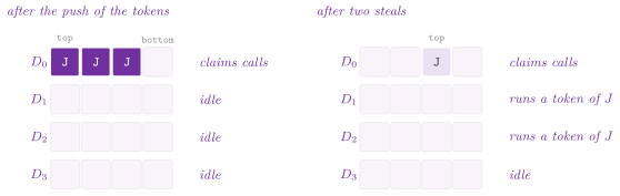
deque of the caller (Figure 25.1). A thread that
runs a token (a thief, or the caller) claims calls from the counter by a
fetch-and-add until none is left. Then it gives the token back by
decrementing \(\mathit{out}\), its last access to the job. Meanwhile, the caller claims calls as well, takes back from the bottom of its deque the tokens that
nobody stole, and waits for \(\mathit{out}\) to reach 0 (Algorithm
25.2). While it waits, it runs the tasks it
steals, and therefore helps a call nested in a call \(f( i )\) of another
thread. Note that no task is allocated: the tasks of the pool are the tokens
of the jobs and the pending calls of invoke(), both on the stacks of the
threads that wait for them.
The public members of the pool are
// declarations of <ADS/parallel/ThreadPool.h>
class ThreadPool
{
 public:
 explicit ThreadPool( std::size_t p = 0 , std::int64_t spin = 2000000 );
 std::size_t concurrency( void ) const;
 template< class F >
 void bulk( std::size_t n , F && f );
 template< class F , class G >
 void invoke( F && f , G && g );
 using lock_type = std::mutex;
 template< class F >
 void run( std::size_t p , F && f );
 };
where \(p = 0\) stands for the hardware threads of the machine, and spin is
the time, in nanoseconds, during which an idle thread looks for work
before it sleeps.
Algorithm 25.2. The bulk() of ThreadPool:
a job of tokens on the deques of Chase and Lev.
In Algorithm 25.2, the procedure \(\mathrm{work}\) is the body of a token. When a call throws, its exception is kept and the counter is set to \(n\), at which the other threads stop claiming (line 13); a thief that runs a token gives it back by a decrement of \(\mathit{out}\) with release, its last access to the job. The take-back of the lines 6 and 7 stops at the first task that is not a token of the job, and pushes it again.
Lemma 25.3. Each deque holds only the tokens
of jobs whose bulk() has not returned and the pending calls of invoke()
that has not returned, in the order in which their calls were entered; hence
the take-back of Algorithm 25.2 takes only tokens
of the job it serves, and a job never outlives the frame that holds it.
Proof. By induction on the calls of one thread, which nest. A call of
bulk() pushes its tokens above what the enclosing calls left on the deque.
A call nested in it (in \(\mathrm{work}( J )\), or in a task that it runs
while waiting) returns before it, having taken back or seen stolen what it
pushed. Hence, when the caller of \(J\) starts the take-back, the bottom of
its deque holds the tokens of \(J\) not stolen, and below them only tasks of
the enclosing calls, at which the loop stops. A token that a thief holds
keeps \(\mathit{out}\) above 0 until it is given back, and bulk() returns
only when \(\mathit{out} = 0\), i.e., after the last access of each thread to
\(J\). \(\square\)
Lemma 25.4. Let the \(n \ge p\) calls of a job cost \(c\) each, and let the thread \(k\) of the pool start claiming them at the instant \(s_k\) after the push of the tokens (\(s_0 = 0\) for the caller). Then the job ends by \(n c / p + c + \frac{1}{p} \sum_k s_k\); if the steals of the tokens follow one another at intervals of \(\sigma\), this is at most \(n c / p + c + ( p - 1 ) \sigma / 2\).
Proof. Let \(t^*\) be the instant of the last claim. As in the proof of Lemma 25.2, a thread that started before \(t^*\) is busy from \(s_k\) to \(t^*\). Hence, \(\sum_k ( t^* - s_k ) \le n c\), i.e., \(t^* \le n c / p + \frac{1}{p} \sum_k s_k\), and the last call ends by \(t^* + c\). Now, the tokens lie on one deque and are stolen from its top one at a time, by a compare-and-swap each; thus, \(s_k \le k \sigma\), whose mean over \(k = 0 , \ldots , p - 1\) is \(( p - 1 ) \sigma / 2\). \(\square\)
The serialized steals of Lemma 25.4 are the price of a job that allocates nothing. One can instead let the thieves spread the tokens over the deques, at the price of a task per thread. With \(p\) in the tens and \(\sigma\) the time of a compare-and-swap on a line that moves between cores, the term is usually small against \(n c / p\) for the jobs of the patterns of §25.6, which have at least a grain of indices per block.
The fork and join. invoke( f , g ) pushes \(g\) as a task on the deque
of the caller and runs \(f\); then it takes \(g\) back and runs it, unless a
thief stole it, in which case it waits for \(g\) while stealing other tasks
(Algorithm 25.3). This is the leapfrogging of
Wagner and Calder 1993: a thread that
waits still works, on tasks that some thread would otherwise run later. If
the take finds a task other than \(g\), the task belongs to an enclosing call
(cf. Lemma 25.3), and it is pushed back for that
call.
Algorithm 25.3. The invoke() of
ThreadPool (Wagner and Calder 1993).
Since the pool schedules by work stealing, we recall the classic bound on the scheduler of Blumofe and Leiserson 1999 from which it derives; the bound is stated for an abstract scheduler, and we say after it which of its hypotheses the pool meets.
Theorem 25.1 (Blumofe and Leiserson). Let a fully strict computation (one in which each join waits only for the tasks forked by its own task) have work \(W\), the number of its unit steps, and depth \(D\), the number of the steps of its longest chain of dependences. Let it be run by \(p\) processors, each of which pushes the tasks it forks at the bottom of its deque and takes them from there, and, when its deque is empty, makes steal attempts at the top of the deque of a victim chosen uniformly at random, independently of the other attempts, each attempt taking one step. Then the expected time is \(W / p + O( D )\), and the expected number of the steal attempts is \(O( p D )\).
Proof. This is the bound on the time and on the steal attempts of the algorithm Work-Stealer of Blumofe and Leiserson 1999, proved there by a delay-sequence argument for fully strict computations under exactly the hypotheses above; a shorter proof by a potential, which weighs each ready task exponentially in the depth left below it and shows that \(p\) consecutive attempts lower the potential by a constant fraction with constant probability, is that of Arora et al. 2001 (their dedicated case). Each step of a processor is a step of work, at most \(W\) in all, or a steal attempt, \(O( p D )\) in expectation, and the \(p\) processors run at once, whence the time \(( W + O( p D ) ) / p\). \(\square\)
The computations of invoke() are fully strict, since invoke( f , g )
joins only the \(g\) that it forked, and the owner and the thieves use the
two ends of the deque as the theorem wants. However, the pool departs from the hypotheses in two points: (i) a thread chooses its first victim by a
generator xorshift, and on a failure tries the other threads in turn rather
than at random; (ii) a thread that waits at a join steals and runs any task
(the leapfrogging), whereas in the computation of the theorem it would stall
or steal under the same rule. We therefore expect, and have not proved,
that Theorem 25.1 holds for the pool. A steal moves the oldest task, which
in a fork and join is the largest; hence, the steals are few when the
parallelism is large, and most tasks run on the thread that made them,
with their data in its cache. The jobs of bulk(), instead, are flat loops on top of it,
balanced as in Lemma 25.4.
25.4 The executors of other runtimes¶
We now turn to the executors that give the same calls to the threads of an external runtime, so that the parallel algorithms of the library run on it unchanged (Algorithm 25.4). We first describe those of FastFlow, OpenMP and oneTBB, then those on the runtimes that a program may already have, which take its threads instead of starting the pool beside them.
FastFlowExecutor keeps a ParallelFor of FastFlow (Aldinucci et al.
2017; Danelutto and Torquati
2014), built at the first call of
bulk() that needs it. Its \(p\) workers schedule the indices in chunks of 1,
since the scheduler thread of FastFlow is disabled (the pool already has as
many workers as threads), and the caller waits without working. Between the
calls the workers spin (a default of the executor) or, if the executor was
built so, sleep. Each call is given all the \(p\) workers and at least \(p\)
indices, those from \(n\) on doing nothing. We do so because of a property of FastFlow, whose spinning workers meet at a barrier of all the workers of the
call, while only those given an index are woken. Furthermore, FastFlow
resets the barrier whenever the number of workers changes from one call to
the next, also while a worker of the previous call may still spin in it. In
both cases the barrier would never be passed; the test
engineered_runtime.fastflow-bulk-sizes checks both.
A ParallelFor does not nest, and therefore a call of bulk() made from
inside a call runs its calls in order on that thread. Two habits of FastFlow
are dealt with by the header. Unless ADS_FASTFLOW_MAPPING is defined, it
defines NO_DEFAULT_MAPPING, since FastFlow would otherwise pin its \(i\)-th
thread to the \(i\)-th core of the machine, whatever the cores given to the
process. It also defines NUM_CORES and NUM_REAL_CORES as functions of
the library that count the processors once, where FastFlow would count the
physical cores by a shell per processor at the construction of each
ParallelFor. These macros reach FastFlow only if the header comes before
all the headers of FastFlow; otherwise the preprocessor stops with an error
that explains the order (the test fastflow-order). For its lock the
executor uses the spin lock of FastFlow, FastFlowLock, whose try_lock()
is one test-and-set of its flag.
OpenMPExecutor runs bulk( n , f ), outside a parallel region, as a loop
#pragma omp parallel for with the dynamic schedule of chunks of 1 on
\(\min\{ p , n \}\) threads, the caller being one of them, as in all the
regions of OpenMP (OpenMP ARB 2021).
Inside a region that is already open (a #pragma omp parallel of the
program around the call, or a call nested in another) a nested region would
get one thread, the default of OpenMP, and the algorithm would run in order
on the caller. The executor makes there a #pragma omp taskloop of chunks of
1 instead, whose calls are tasks of the team in place and whose implicit
taskgroup waits for them, the waiting thread running tasks meanwhile. Hence
the threads are those of the team, which concurrency() gives when the
executor is built with \(p = 0\), and the calls nest as the tasks of OpenMP
do; we remark that the mode needs OpenMP 4.5, which MSVC has only with
/openmp:llvm. Its invoke() is bulk() on 2 indices. Its lock is
omp_lock_t (the class OpenMPLock), built on the runtime of LLVM with the
hint omp_sync_hint_uncontended, which that runtime realizes as a
test-and-set lock. In fact, the default lock of the runtime of LLVM queues
the threads and hands over in their order; with more threads than cores the
next owner is often descheduled, and the others wait behind it (libgomp
ignores the hint).
TBBExecutor runs in a task_arena (Reinders
2007; Voss, Asenjo and Reinders
2019), of one of three kinds. It may own an
arena of \(p\) threads; it may refer to an arena of the program without owning
it, and then the constraints of that arena (its NUMA node, its type of core,
its priority and its number of threads) hold for the calls of the library
too; or it may take, at each call, the arena of the calling thread, which is
the arena of the loop of oneTBB from which the program calls an algorithm of
the library. The arenas of a process share the workers of oneTBB, and
therefore none of the three starts threads, while the caller joins the arena
as one more thread. Its bulk() is a parallel_for of oneTBB with the
simple partitioner, i.e., a task per index (the patterns of the library
already cut the loop into blocks), and its invoke() is parallel_invoke,
both in the arena; its calls nest as the tasks of oneTBB do.
As to their interface, the three classes have the members of ThreadPool but
for their constructors, explicit FastFlowExecutor( std::size_t p = 0 , bool
spin = true ), explicit OpenMPExecutor( std::size_t p = 0 ) and explicit
TBBExecutor( std::size_t p = 0 ), with explicit TBBExecutor(
tbb::task_arena & arena ) for an arena of the program and explicit
TBBExecutor( Current ) for the current one (by the tag
TBBExecutor::current), and for their lock_type (FastFlowLock,
OpenMPLock and tbb::spin_mutex). FastFlowExecutor has no invoke(),
and parallelInvoke() runs its two calls by bulk() on two indices, as for
any executor without it.
A program that already runs on another runtime usually wants the algorithms
of the library on its threads, since the pool would compete with them and
spin for 2 ms after each call (as libgomp and oneTBB do after theirs). The
headers of ADS/interop/parallel/ give four more executors for this purpose.
Each is compiled where the headers of its runtime are found.
StdParExecutor< Policy > runs bulk( n , f ) as std::for_each( Policy()
, first , last , g ) on the indices, with std::execution::par by default.
Its threads are then those of the backend of the standard library, e.g.,
oneTBB under libstdc++, the pool of MSVC or the threads of nvc++
-stdpar=multicore. We take the indices from an iterator of the library, since
those of std::views::iota are only input iterators of C++17. The standard
has no query of the threads of a policy either, and concurrency() is the
number given to the constructor. SenderExecutor< Sch > runs bulk() as
the sender schedule( s ) | bulk( par , n , f ) of a scheduler, waited by
sync_wait(), on stdexec, the implementation of reference of the senders
and the receivers of C++26 (Dominiak et al.
2024). TaskflowExecutor runs it as a
graph of Taskflow (Huang et al. 2022)
made of one for_each_index, run and waited from a thread outside the
executor of Taskflow and co-run from one of its workers, which keeps running
tasks while it waits. KokkosExecutor< Space > runs it as a
Kokkos::parallel_for on a space of the host (Trott et al.
2022), followed by the fence() of the
space; the spaces of the devices do not fit, since the calls of the library
run code of the host on memory of the host.
These four executors do not come at the same price. On oneTBB, on OpenMP and
on the parallel algorithms of the standard library the executor adds no cost
to the call of the runtime but the execute() of an arena, and the calls
nest as the tasks of the runtime do. A sync_wait() of the senders and a
dispatch of Kokkos hold instead the thread that waits, and Kokkos forbids a
dispatch from inside a kernel. Thus a call of bulk() made inside a call of
these two executors, or inside a kernel of the program, runs its calls in
order on its thread, which the contract of
§25.2 allows. In this case the fork and join of
the library (the recursion of parallelInvoke(), the trees by join, the
lower levels of the sorts) loses its nested parallelism, while the loops, the
reductions, the prefix sums and the top level of the sorts keep theirs.
Taskflow nests. Its cost is a graph with its nodes on the heap at each call
of bulk(), which the patterns of the library make once per loop of at most
kBlocks indices. None of the four has run(), since their runtimes
do not promise that the calls of a loop run at the same time; the
long-lived workers of §25.5 need one of the
other executors.
Their constructors are explicit StdParExecutor( std::size_t p = 0 ),
SenderExecutor( Sch s , std::size_t p ), explicit TaskflowExecutor(
tf::Executor & e ) and explicit KokkosExecutor( Space s = Space() ), and
their other members are concurrency() and bulk(). With CMake each
runtime found gives a target (ADS::StdPar, ADS::stdexec,
ADS::Taskflow or ADS::Kokkos) with the macro of the header, the runtime
and ADS::ADS, a component of the installed package as well (cf.
find_package( ADS COMPONENTS Taskflow )). Since ADS::ADS carries none
of them, a program takes a runtime only by linking its target. The
options ADS_WITH_STDPAR, ADS_WITH_STDEXEC, ADS_WITH_TASKFLOW and
ADS_WITH_KOKKOS are AUTO, and off in the packages. We run the tests of the
parallel algorithms on all the executors found, those of the runtimes
included, against the results of Sequential (engineered_parallel,
engineered_speculative and interop_parallel).
Algorithm 25.4. The bulk() of
FastFlowExecutor, OpenMPExecutor and TBBExecutor, and of the executors
on the runtimes of a program.
25.5 Long-lived workers¶
We recall that the calls of bulk( n , f ) are tasks: an executor may run several of them
on one thread, one after the other, and a call starts only when a thread is
free to take it. A call that waits for another one (at a barrier, or for a
message) may therefore wait forever for a call that no thread will start
before it returns. Consider instead a computation of workers, each a loop
that lives as long as the computation and talks to the others, as the
workers of a parallel search or the master and the workers of a farm. Such a
computation needs its \(p\) calls to run at the same time on \(p\) distinct
threads. For this purpose, the concept WorkerExecutor of Executor.h adds this to
Executor: run( p , f ) runs \(f( 0 ) , \ldots , f( p - 1 )\) at the same
time on \(p\) distinct threads, and lock_type is the mutex that the executor
prefers for the short sections that the workers share. Each lock_type is
Lockable in the sense of the standard, i.e., it has try_lock() besides
lock() and unlock(), which takes the lock only if it is free and never
waits. A worker that finds a shared section busy (the update of a common
bound, the publication of a part of its work) may then skip it and come back
later, instead of queueing behind the holder. Table
25.3 summarizes how each executor meets the
requirement.
Table 25.3. How each executor runs the \(p\)
calls of run( p , f ), why they run together, and its lock.
| Executor | The calls | Why they run together | lock_type |
|---|---|---|---|
Sequential |
\(f( 0 )\) on the caller, \(p \le 1\) | one worker | std::mutex |
ThreadPool |
\(f( 0 )\) on the caller, the others claimed one each under a mutex by the workers idle in their loop | a thread that waits inside a call never claims one (Lemma 25.5) | std::mutex |
OpenMPExecutor |
a region omp parallel of \(p\) threads, \(f( i )\) on its thread \(i\) |
the team has \(p\) threads, or nothing runs and run() throws |
OpenMPLock (omp_lock_t) |
TBBExecutor |
a parallel_for of the arena, a task per call, each inside isolate() |
a thread that waits inside a call takes only the tasks of the jobs nested in it | tbb::spin_mutex |
FastFlowExecutor |
a parallel_for of a second ParallelFor on \(p\) workers, chunks of 1 |
each worker is given its own index first | FastFlowLock (ff::lock_t) |
Algorithm 25.5. The run() of ThreadPool;
\(c\) is the next call to claim and \(d\) the number of the calls of the workers
that have returned.
Lemma 25.5. Let a ThreadPool have \(p - 1\)
workers idle in their loop besides the thread that calls run( p , f ).
Then the \(p\) calls run at the same time on distinct threads, whatever the
calls do, nested jobs included.
Proof. The caller makes \(f( 0 )\). All the other calls are claimed one at a time from a counter under a mutex, only by a worker that is in its loop, i.e., that holds no call of any job. A worker that has claimed a call goes back to its loop only after the call has returned, and therefore no thread holds two calls of the run. A thread that waits inside a call, for a job nested in it or for the end of the run, steals and runs only tasks, never a call of the run (were it to run one, it would hold it below the call it is in, which might wait for it forever). Hence, the \(p - 1\) idle workers claim the \(p - 1\) calls, one each, as soon as the event count of the pool wakes them, and all the calls run together. \(\square\)
On the other executors the same property rests on the runtime. Thus, the team of a region of OpenMP has its \(p\) threads from the start; a runtime that gives
the region fewer threads (a run nested in a region, or a limit on the
threads) makes run() throw before any call, since the workers could not
all run together. A thread of oneTBB inside isolate() takes only the tasks
spawned within it, and the arena has \(p\) threads when the threads of oneTBB
are not fewer, i.e., for \(p\) not larger than the hardware threads. The
ParallelFor of FastFlow cuts \([ 0 , p )\) into \(p\) chunks of 1, one per
worker. A worker looks at the chunks of the others only after the chunk of
its index, and thus takes the call of another only when the call of its
index has returned. Moreover, the workers of this second ParallelFor sleep between
the runs, and those of bulk() are put to sleep before a run. In fact,
threads that spin unpinned may share a core with the thread that the run
waits for, which would then lose a quantum of the scheduler of the system.
Algorithm 25.6. The run() of
FastFlowExecutor, OpenMPExecutor and TBBExecutor.
Placement of the threads. A worker that is moved by the system to
another processor finds there cold caches, and on a machine of several
sockets the pages it touched first stay on the node of the old one (the
policy of the first touch; Drepper 2007,
§6.4). Affinity.h gives the processors
on which the process may run, affinityCpus(), as the first call found them
(those left by taskset or numactl, in increasing order). Then
pinThread( i ) binds the calling thread to the processor \(i \bmod c\) of
them, \(c\) their number (Algorithm 25.7); the
workers \(0 , 1 , \ldots\) of a pool that call it at their start thus fill
those processors in order. The placement is that of hwloc (Broquedis et
al. 2010), with ADS_WITH_HWLOC,
which reads and sets the binding of a thread on each system in its own way;
without hwloc affinityCpus() is empty, availableCpus() falls back on
std::thread::hardware_concurrency(), and pinThread() returns false.
Also, currentCpu() gives the processor on which the calling thread runs
now (the last one that hwloc saw, and \(-1\) without hwloc). No
executor pins its threads, since two programs pinned to the same processors
would slow each other down, and the choice is left to the caller.
The four functions of Affinity.h are
// declarations of <ADS/parallel/Affinity.h>
const std::vector< int > & affinityCpus( void );
unsigned availableCpus( void );
bool pinThread( unsigned i );
int currentCpu( void );
Algorithm 25.7. The binding of the calling thread to a processor.
A worker that pins its thread must not pin the thread of the caller, which
goes on after the run with the placement that the program gave it, and
isRunCaller(), called in a call, returns whether it runs on that thread.
On Sequential, ThreadPool and OpenMPExecutor the caller makes \(f( 0 )\)
(the thread 0 of a region of OpenMP is the thread that opens it). It makes
none of the calls on FastFlowExecutor with \(p > 1\), where it only waits,
and any one of them or none on TBBExecutor, where it joins the arena as
one more thread. Since the calls run on distinct threads, the caller holds
at most one of them; the mark is a variable of the thread, set for the time
of the run, which a call reads by one load.
25.6 Loops, reductions and prefix sums¶
The blocks of a loop on \([ \mathit{first} , \mathit{last} )\) depend only on
the number \(n\) of its indices and on the grain \(g\), never on the threads: \(s
= \max\{ g , \lceil n / \mathit{kBlocks} \rceil \}\) indices per block and
\(\lceil n / s \rceil\) blocks (Algorithm 25.8).
parallelForBlocks() gives each block to one call f( lo , hi ), so that
the compiler sees a loop that it can vectorize, and parallelFor() makes of
it the call f( i ) per index; the blocks are the calls of one bulk(),
which the executor schedules as in Lemma 25.2 or
as its runtime does.
These patterns, and the scans below, are declared as
// declarations of <ADS/parallel/Executor.h>
inline constexpr std::size_t kGrain = 1024;

std::pair< std::size_t , std::size_t >
blocksOf( std::size_t first , std::size_t last , std::size_t grain = kGrain );
template< Executor E , class F >
void parallelForBlocks( E & ex , std::size_t first , std::size_t last ,
                        F && f ,
                        std::size_t grain = kGrain );
template< Executor E , class F >
void parallelFor( E & ex , std::size_t first , std::size_t last , F && f ,
                  std::size_t grain = kGrain );
template< Executor E , class T , class F , class Op >
T parallelReduce( E & ex , std::size_t first , std::size_t last , T id ,
                  F && f ,
                  Op op , std::size_t grain = kGrain );
template< Executor E , std::random_access_iterator I ,
          std::random_access_iterator O , class T , class Op = std::plus<> >
T parallelInclusiveScan( E & ex , I in , std::size_t n , O out , T init ,
                         Op op = Op() );
template< Executor E , std::random_access_iterator I ,
          std::random_access_iterator O , class T , class Op = std::plus<> >
T parallelExclusiveScan( E & ex , I in , std::size_t n , O out , T init ,
                         Op op = Op() );
and they combine, e.g., into a loop, a sum and a sort on the same pool:
ADS::ThreadPool pool( 4 );
std::vector< double > x( 1000000 );
ADS::parallelFor( pool , 0 , x.size() ,
                  [ & ]( std::size_t i ) { x[ i ] = double( i % 1000 ); } );
double s = ADS::parallelReduce(
  pool , 0 , x.size() , 0.0 ,
  [ & ]( std::size_t lo , std::size_t hi ) {
   double r = 0;
   for( std::size_t i = lo ; i < hi ; ++i )
    r += x[ i ];
   return( r );
   } ,
  std::plus<>() );     // s is 499500000
ADS::sort( pool , x );  // of ParallelSort.h
Algorithm 25.8. The blocks of a loop, the loop on the blocks and the loop on the indices.
parallelReduce() reduces each block by f( lo , hi ) into a partial
result, in parallel, and combines the partial results by \(\oplus\) in the
order of the blocks on the calling thread (Algorithm
25.9), so that its result is
Algorithm 25.9. The reduction by blocks.
Lemma 25.6. The result of parallelReduce()
is (25.3) on all the executors and for any number of threads, Sequential
included, also when \(\oplus\) is associative only up to rounding (e.g., the
sum of floating point numbers); when \(\oplus\) is associative, it is the
reduction from left to right. Its work is \(O( n )\) and its depth \(O( n / B +
B )\).
Proof. By construction, the blocks are those of Algorithm 25.8, which depend on \(n\) and \(g\) only. Each \(r_b\) is computed by one call, in the order of \(f\), and the partial results are combined in one fixed order; the second statement is the associativity. A block has \(O( n / B )\) indices, and the combination costs \(B\) operations. \(\square\)
It is fair to remark that the result of Lemma
25.6 is the sum by blocks, which on floating point
numbers may differ in the last bits from the sum of std::accumulate();
what the lemma ensures is that it does not depend on the executor.
Prefix sums. The prefix sums \(y_i = x_0 \oplus \cdots \oplus x_i\) (or up
to \(x_{i - 1}\), the exclusive ones) are the pattern of the counting sorts,
of the compaction of a vector and of the distribution of the parallel sort.
In this respect, the scan of Blelloch 1990 reduces the
blocks, scans the \(B\) partial results and then scans each block from its
prefix. It reads the input twice and writes the output once, i.e., \(3 n\)
moves of the memory. parallelInclusiveScan() and parallelExclusiveScan()
do it in one pass by the decoupled look-back of Merrill and Garland
2016a, written for the processors
instead of the graphics cards. Here we cut the input into tiles of about 64 KB
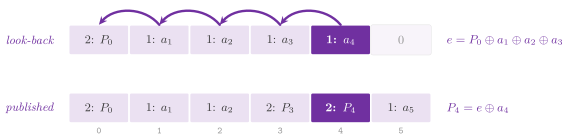
(at least 256 items), which the threads claim in increasing order from a counter. A thread reduces its tile \(c\) into its aggregate \(a_c\), which
leaves the tile in its cache, and publishes it with the flag 1. Then it
looks back at the tiles before it: from \(c - 1\) down, it adds on the left
the aggregate of each tile that has published only that, and stops at the
first one that has published its inclusive prefix \(P_{c'}\) (the flag 2).
Thus,
then it publishes \(P_c\) and writes the prefixes of its tile, reading it again from the cache (Algorithm 25.10, Figure 25.2). In all, the input is read from the memory once and the output written once, \(2 n\) moves. On one thread, or when the input fits one tile, the scan is a single sequential pass.
Algorithm 25.10. The inclusive and the exclusive scans by decoupled look-back (Merrill and Garland 2016a); the second differs in its line 16 only.
The look-back is the core of the scan; a tile whose call has failed publishes the flag 3, at which the tiles after it stop instead of waiting in the line 11 of Algorithm 25.10.
Lemma 25.7. The scan by decoupled look-back ends on any executor, also on one that runs its calls one after the other, and its prefixes are those of the scan from left to right.
Proof. A thread waits only for a tile before the one it holds, and the tiles are claimed in increasing order. Hence, a tile before \(c\) is held by a thread that runs, which claimed it before \(c\) was claimed. Then the least tile not done waits for no tile, since all the tiles before it have published their prefix; by induction on the tiles, each tile is done, also when the threads are fewer than the tiles or when one thread runs all of them in order. Also, the flags are stored with release after the values they announce and loaded with acquire before these are read, and therefore a value is read whole. Finally, the prefixes are right by (25.4) and the associativity of \(\oplus\), since the tiles added on the left are those after the last prefix met. \(\square\)
The look-back reads \(O( 1 )\) tiles on average when the threads go at the same pace, since the tile before is then about to publish its prefix, and at most \(c\) tiles. Unlike the reduction, the scan groups the operations by the tile at which each look-back stops, which depends on the timing of the threads. Hence, the prefixes are those of the scan from left to right only for an associative \(\oplus\); on floating point numbers they may differ from run to run in the last bits.
25.7 Merging and sorting¶
The parallel merge. multiwayMerge( ex , R , out , less ) of
ParallelMerge.h writes into out what the sequential multiwayMerge()
writes, i.e., the items of \(k\) sorted ranges \(R_1 , \ldots , R_k\), \(N\) in
all, in the order of the stable merge (on equal items the range of lower
index first). We cut the output into \(B = 4 p\) parts of about \(N / B\) items
(at least \(2^{14}\) each), and the sequential merge writes each part into its
place, in parallel. Their correctness rests on the following property of the
stable merge (Varman et al. 1991).
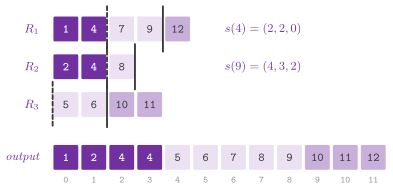
Lemma 25.8. Order the items by the triples \(( \mathit{item} , \mathit{range} , \mathit{position} )\). For each rank \(r \le N\) there is a unique split \(s( r ) = ( s_1( r ) , \ldots , s_k( r ) )\), with
such that the first \(s_i( r )\) items of each range \(i\) are the \(r\) least items, and the stable merge writes them, in its order, before the others.
Proof. We observe that the order of the triples is total and, within a range, it is the order of the positions, since the range is sorted. Hence, the \(r\) least triples form a prefix of each range, unique, and the lengths of the prefixes sum to \(r\). Also, the order of the triples is that of the stable merge, which on equal items takes the range of lower index first. \(\square\)
The part \(q\) of the output is then the merge of the pieces \([ s_i( r_q ) ,
s_i( r_{q + 1} ) )\) of the ranges, written from the rank \(r_q\), and the
parts are independent (Figure 25.3).
multisequenceSplit() finds \(s( r )\) by narrowing a window \([ \mathit{lo}_i
, \mathit{hi}_i )\) on each range (Algorithm
25.11). Its invariant is that the items before
\(\mathit{lo}_i\) are among the \(r\) least and those from \(\mathit{hi}_i\) on
are not. At each step, the pivot \(x\) is the middle item, at the position \(m\), of the
window of a range \(j\), chosen as the weighted median of the middles of the
windows by their widths. A binary search in each window counts the items
before \(( x , j , m )\), those \(\le x\) in the ranges \(i < j\) and those \(< x\)
in the ranges \(i > j\). If they are fewer than \(r\), \(x\) and all of them go to
the left, otherwise to the right.
The two functions are declared as
// declarations of <ADS/parallel/ParallelMerge.h>
template< std::random_access_iterator I , class C = std::less<> >
std::vector< std::size_t >
multisequenceSplit( const std::vector< std::pair< I , I > > & R ,
                    std::size_t r ,
                    C less = C() );
template< Executor E , std::random_access_iterator I ,
          std::random_access_iterator O , class C = std::less<> >
O multiwayMerge( E & ex , const std::vector< std::pair< I , I > > & R , O out ,
                 C less = C() );
Algorithm 25.11. The multisequence selection and the parallel merge (Varman et al. 1991).
Lemma 25.9. Each step of
multisequenceSplit() removes at least a quarter of the total width of the
windows; hence a split takes \(O( \log N )\) steps, i.e., \(O( k ( \log N +
\log k ) \log N )\) comparisons.
Proof. Let \(w\) be the total width, and order the windows by their middles \(( R_i[ m_i ] , i )\). By definition, the median \(j\) is the first window at which the widths summed in this order reach \(w / 2\); hence, the windows up to \(j\) weigh at least \(w / 2\), and so do those from \(j\) on. Let \(x\) go to the left. A window \(i\) whose middle is not after \(( x , j )\) has \(R_i[ m_i ] \le x\) if \(i < j\) and \(R_i[ m_i ] < x\) if \(i > j\), and therefore its count is past \(m_i\). Its \(\mathit{lo}_i\) thus rises past the middle, and it loses at least half of its width. The other case is symmetric, with \(\mathit{hi}_i\) falling to the middle for the windows from \(j\) on. Now, the total width starts at \(N\), is an integer and shrinks by a factor of at least \(3/4\) at each step, and it is 0 after at most \(\log_{4/3} N + 1\) steps. Each step costs \(k\) binary searches, \(O( k \log N )\) comparisons, and a sort of \(k\) middles, \(O( k \log k )\). \(\square\)
The splits are found in parallel, one per part, and cost far less than the merge, which makes \(O( N \log k )\) comparisons; with \(B = 4 p\) parts the merge takes \(O( ( N / p ) \log k )\) time plus the splits. The bound of Lemma 25.9 is that of the selection of Varman et al. 1991 up to a factor \(\log k\), which the simpler choice of the pivot costs.
The parallel sorts. sort( ex , A , less ) and
stableSort( ex , A , less ) of ParallelSort.h give the result of the
sequential sorts of the library, which they call on the parts they cut \(A\)
into. With fewer than kParallelSortThreads \(= 3\) threads, or fewer than
kParallelSort \(= 2^{15}\) items, they are those sequential sorts; on 2
threads, in fact, the passes of the distribution cost more than the second
thread saves. Their procedure is the samplesort of Sanders and Winkel
2004 as engineered in IPS4o (Axtmann et
al. 2022), preceded by two surveys of the
input (Algorithm 25.12).
The four sorts of ParallelSort.h are declared as
// declarations of <ADS/parallel/ParallelSort.h>
template< Executor E , class T , class C = std::less<> >
void sort( E & ex , std::vector< T > & A , C less = C() );
template< Executor E , class T , class C = std::less<> >
void stableSort( E & ex , std::vector< T > & A , C less = C() );
template< Executor E , VectorKey T >
void learnedSort( E & ex , std::vector< T > & A );
template< Executor E , VectorKey T >
void learnedStableSort( E & ex , std::vector< T > & A );
where VectorKey admits the integers and the floating point numbers
(chapter 12).
Algorithm 25.12. The parallel sorts; the recursion of line 18 is at most 3 deep.
We first run a parallel reduction by blocks. It finds whether \(A\) is sorted (then no item moves) or in decreasing order (strictly, for the stable sort; then it is reversed in parallel), by stretches of 32 pairs with no branch inside, which vectorize. A block stops at the first stretch out of both orders, and on most inputs the pass therefore reads little. Then a second survey cuts each of 8 blocks (or \(p\), if more) into its maximal runs, non-decreasing or strictly decreasing, and gives up at the ninth run of a block. If no block gave up, \(A\) is made of at most 8 runs per block. Its decreasing runs are reversed, and all the runs are merged stably by the parallel merge above through a buffer, in \(O( ( n / p ) \log r )\) time for \(r\) runs, where a distribution would forget that order.
Otherwise the items are distributed into \(k\) buckets whose concatenation is
sorted, by one of two classifiers. Let the items be numbers in their natural
order, and let \(\ell\) and \(u\) be the least and the greatest key of a sample
of 1024 items (the keys of radixKey(), with \(-0\) taken as \(+0\)). Then the
bucket of \(x\) is
with \(s\) the least shift that leaves at most 256 buckets, i.e., the 8 highest bits in which the keys of the sample differ; the keys out of the range of the sample go to the two buckets at the ends. We remark that the bits spread the keys only when the keys are spread, which is not the case of the floating point numbers of a few exponents, or of the integers of a law with a heavy tail. If a bucket gets more than 4 times its share of the sample (and 32 more), the numbers go to the other classifier. When the sample shows at most 32 distinct values that the bits do not separate, the numbers are counted instead (but by the stable sort of floating point numbers, whose \(-0\) and \(+0\) are equal and yet differ). Each is found among those values by counting the keys less than its key (32 comparisons in vectors), and \(A\) is filled with them in order, in 2 passes over \(A\); an item of another value sends \(A\) to the other classifier. Any other item is classified by \(k - 1\) splitters taken from a sorted random sample of \(16 k\) items, an oversampling that keeps the buckets within a small factor of \(n / k\) with high probability. These splitters lie in an implicit binary tree, which a search descends with no branch. If the sample repeats a splitter, the items equal to each splitter go to a bucket that needs no sort (the buckets of equality of IPS4o), and therefore \(k\) distinct keys cost \(O( n \log k )\). In both cases \(k\) is 256 for \(n \ge 2^{20}\), and otherwise the larger of \(4 p\) rounded up to a power of 2 and \(n / 4096\) rounded down to one (at most 256 for the comparisons).
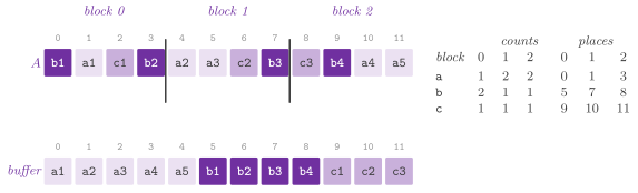
In all cases, the distribution is a parallel loop on \(B\) blocks of \(A\), each counting its items per bucket; when the classifier compares, the bucket of each item is kept, and an item is classified once. Then the prefix sums of the counts in the order (bucket, block) give each block the place of its items of each bucket in a buffer of \(n\) items, and a second parallel loop moves them there (Figure 25.4); the prefix sums are those of the line 16 of Algorithm 25.12, computed on one thread over the \(k B\) counts.
Lemma 25.10. The distribution is stable: two items of one bucket keep in the buffer the order they had in \(A\).
Proof. By construction, the prefix sums in the order (bucket, block) give the places of a bucket to the blocks in their order, and a block moves its items in their order to consecutive places. Two items of one block thus keep their order, and an item of an earlier block goes before the items of a later block in the same bucket. \(\square\)
Items copied as bytes, several to a line of the cache, go first to a line of
64 bytes per bucket on the stack of the thread, which is copied to the
buffer when full (the software write-combining of the radix sorts). In this way, the \(k\) streams of stores leave whole lines, instead of reading each line of
the buffer before writing an item into it. This buffer comes from
Scratch.h, which keeps on huge pages the block of the last call that gave
its room back, and gives it to the next call if it is large enough
(Algorithm 25.13). A fresh block costs, in the
faults that clear its pages, about as much as the moves of the items into
it, while the pages of a block already used are faulted in. A call that
finds the block taken by another call allocates a new one.
Algorithm 25.13. The room of the parallel algorithms, a cache of one entry.
Last, the threads claim the buckets from the largest down, the schedule LPT of Graham 1969, within \(4 / 3\) of the best on identical threads. A thread moves its bucket into a vector, sorts it by the sequential sort and moves it into its place in \(A\). A bucket of numbers of 32 or 64 bits in their natural order goes instead straight to its place, where the quicksort in the vector registers sorts it, unless a scan finds it already in order or made of few runs; a bucket of equal items is moved back as it is. A bucket larger than \(n / p\), which one thread would take too long on, is sorted first by the same parallel sort on all the threads, down to a depth of 3 recursions. With \(n\) items and \(p\) threads the sort moves each item about 4 times and makes \(O( n \log k )\) comparisons to classify. We bound the time by \(O( n / p + k p )\) for the classification (the counts are \(k B\) words) and \(O( ( n / p ) \log( n / k ) )\) for the buckets, when they are balanced.
The learned sorts learnedSort( ex , A ) and learnedStableSort( ex , A )
change the classifier only (Algorithm 25.14). On
numbers of 32 or 64 bits, the bucket of a key is read from a model of the
distribution function of a sample of 4096 keys (Kristo et al.
2020), a grid whose cell leaves 4
comparisons with no branch instead of the 8 dependent steps of the tree. If
the sample shows a distribution that the model does not fit, the sort falls
back on the classifiers above. Note that sort( ex , A ) does not use the
model unless one requests it, since on the measures made so far it did not beat the
bits and the tree beyond the noise of the machine.
Algorithm 25.14. The learned parallel sorts (Kristo et al. 2020).
25.8 Products of matrices¶
ParallelNumeric.h computes the products by a vector of the sparse matrices
CsrMatrix and SellMatrix, and the product of dense matrices of gemm(),
with the results of the sequential products bit for bit: each entry of the
output is computed by the same sequential code, with the same order of the
sums, by one thread. Consider a CsrMatrix (or a BasicCsrMatrix of any
types of values and indices) of \(m\) rows and \(\mathit{nnz}\)
nonzeros, with \(\mathit{start}( i )\) the first nonzero of the row \(i\). A row
costs its nonzeros plus the store of its sum, and therefore the rows before
\(i\) cost \(i + \mathit{start}( i )\), which grows with \(i\). Hence, the rows
are cut into \(B = \min\{ 4 p , m \}\) parts of equal \(m + \mathit{nnz}\), each
bound found by a binary search on that quantity, and each part is multiplied
on one thread (Algorithm 25.15). These bounds
are the diagonals of the merge path of Merrill and Garland
2016b, applied to whole rows.
The products are declared as
// declarations of <ADS/parallel/ParallelNumeric.h>
template< Executor E , class T , std::integral I , std::integral P >
void multiply( E & ex , const BasicCsrMatrix< T , I , P > & A , const T * x ,
               T * y );
template< Executor E , class T , std::integral I , std::integral P >
std::vector< T > multiply( E & ex , const BasicCsrMatrix< T , I , P > & A ,
                           const std::vector< T > & x );
template< Executor E , std::size_t C >
void multiply( E & ex , const SellMatrix< C > & A , const double * x ,
               double * y );
template< Executor E , std::size_t C >
std::vector< double > multiply( E & ex , const SellMatrix< C > & A ,
                                const std::vector< double > & x );
template< Executor E , class T >
void gemm( E & ex , std::size_t m , std::size_t n , std::size_t k , T alpha ,
           const T * A , std::size_t lda , const T * B , std::size_t ldb ,
           T beta ,
           T * C , std::size_t ldc );
template< Executor E , class T >
DenseMatrix< T > multiply( E & ex , const DenseMatrix< T > & A ,
                           const DenseMatrix< T > & B );
Algorithm 25.15. The product of a sparse matrix by rows by a vector, in place and as a new vector, and the same for a matrix by chunks of \(C\) rows.
Lemma 25.11. Each part of the product of a
CsrMatrix costs less than \(( m + \mathit{nnz} ) / B + 1 + \ell\), where
\(\ell\) is the largest number of nonzeros of a row.
Proof. Let \(\phi( i ) = i + \mathit{start}( i )\), \(T = m + \mathit{nnz}\) and \(t_q = \lfloor q T / B \rfloor\), and let the part \(q\) be the rows \([ r_0 , r_1 )\), nonempty (an empty part costs nothing). Here the binary searches give the first rows with \(\phi \ge t_q\) and \(\phi \ge t_{q + 1}\), whence \(\phi( r_0 ) \ge t_q\) and \(\phi( r_1 - 1 ) \le t_{q + 1} - 1\), the values being integers. Hence the cost of the part is \(\phi( r_1 ) - \phi( r_0 )\), where \(\phi( r_1 ) = \phi( r_1 - 1 ) + 1 + \ell_{r_1 - 1}\), \(\ell_i\) the nonzeros of the row \(i\); hence it is at most \(t_{q + 1} - t_q + \ell \le \lceil T / B \rceil + \ell < T / B + 1 + \ell\). \(\square\)
A row is never split among threads, which would change the order of its
sums; a row longer than a part thus forms a part with no other row, and usually only a
matrix with a few rows holding most of the nonzeros is unbalanced. A
SellMatrix is cut in the same way, its chunks of \(C\) rows taking the place
of the rows and their places, padding included, that of the nonzeros. Note
that the product moves \(12 \mathit{nnz} + 8 ( m + n )\) bytes (a value of 8
bytes and a column of 4 per nonzero, and the vectors \(x\) and \(y\)) for \(2
\mathit{nnz}\) operations. It is thus bound by the bandwidth of the memory,
and \(p\) threads gain at most the ratio of the bandwidth of the socket to
that of one core.
Unlike the sparse one, the product of dense matrices is bound by the operations, \(2 m n k\)
for \(C \gets \alpha A B + \beta C\) (Algorithm
25.16). With the backend of a CBLAS it is one
call of the CBLAS from the calling thread, as in the sequential gemm(). In
fact, the CBLAS runs on threads of its library (e.g., those of
OPENBLAS_NUM_THREADS), and the threads of both would multiply each other;
the result is that of the sequential call, as it is the same call. Without a
CBLAS, each of \(t = \min\{ p , m \}\) threads takes a range of the rows of
\(C\), as evenly as they go. It computes them by the loops of the sequential
product, blocked so that a block of \(B\) stays in the cache while the rows of
\(C\) run over it, and the sum of an entry runs in the order of the common
index on any split of the rows. We remark that the threads do not share a
packed panel of \(B\), as the many-threaded products of Smith et al.
2014 do: each thread reads the whole \(B\),
which costs bandwidth that a CBLAS saves.
Algorithm 25.16. The product of dense matrices.
25.9 Visits of graphs and the LCP array¶
The visit in breadth. The levels of a visit in breadth from \(s\) are
and a node of \(L_\ell\) is at distance \(\ell\) from \(s\).
bfsDistances( ex , g , s , gt ) of ParallelGraph.h builds each level of a
StaticGraph by (25.7) in either of two directions (Beamer, Asanović and
Patterson 2012). From the top down, the
nodes of the frontier \(L_\ell\) claim their neighbors not yet reached, by a
compare-and-swap of the distance from \(-1\) to \(\ell + 1\). Then the nodes
claimed by the blocks of the frontier are gathered into the next frontier,
each block keeping in a vector of its own the nodes that it claimed and the
sum of their degrees, which gives \(m_f\) for the next level.
From the bottom up, each node not yet reached looks among the arcs into it
for one whose tail is in the frontier, kept as a bitmap, and stops at the
first it finds. We let the visit go from the bottom up when the arcs out of the
frontier \(m_f\) exceed the arcs still to check \(m_u\) divided by \(\alpha =
15\), which typically happens on the few large levels of the graphs of small
diameter (e.g., the social networks). It goes back from the top down when
the frontier shrinks below \(n / \beta\), \(\beta = 18\) (Algorithm
25.17). From the bottom up, a step reads the arcs
into each node, i.e., those of \(g\) if it is unoriented and those of its
transpose gt if it is oriented; with no transpose an oriented graph is
visited from the top down only.
The two algorithms on graphs are declared as
// declarations of <ADS/parallel/ParallelGraph.h>
template< Executor E , class W , ArcLayout AL >
std::vector< int >
bfsDistances( E & ex , const StaticGraph< W , AL > & g , int s ,
              const StaticGraph< W , AL > * gt = nullptr );
template< Executor E , class W , ArcLayout AL >
std::vector< int >
connectedComponents( E & ex , const StaticGraph< W , AL > & g );
Algorithm 25.17. The visit in breadth that optimizes its direction (Beamer, Asanović and Patterson 2012).
Lemma 25.12. Both directions build the
level \(L_{\ell + 1}\) of (25.7), whatever the order of the threads; hence
bfsDistances() gives the distances of the sequential visit. With \(k\)
steps from the bottom up its work is \(O( ( n + m ) ( 1 + k ) )\), and its
depth is \(O( D \log n )\) on a graph of eccentricity \(D\) from \(s\), but for
the depth of the claims of a node of large degree.
Proof. From the top down, a node \(v\) not yet reached with a neighbor in \(L_\ell\) is claimed by some arc, since the claims fail only on the nodes already reached. Moreover, the compare-and-swap succeeds for one claimant only, which writes \(\ell + 1\) whoever it is, and a node of an earlier level keeps its distance. From the bottom up, a node not yet reached enters the level if and only if one of its arcs comes from the bitmap of \(L_\ell\), which is fixed during the step. As to the costs, from the top down each node enters one frontier, and the arcs out of it are read once, at that step; the steps from the top down thus read \(O( n + m )\) in all. A step from the bottom up scans all the \(n\) nodes and reads at most all the \(m\) arcs into them, hence \(O( n + m )\) each and \(O( ( n + m ) k )\) for \(k\) of them. There are at most \(D + 1\) levels, and each step is a parallel loop over the frontier or over the nodes, followed by the gathering of the blocks, a prefix sum of depth \(O( \log n )\); the loop over the arcs of one node runs on one thread, whence the proviso on the degrees. \(\square\)
The two directions thus differ in the arcs they read: from the top down the arcs out of the frontier, and from the bottom up those into the nodes not yet reached, up to their first hit; the thresholds \(\alpha\) and \(\beta\) keep \(k\) to the few large levels where these steps read fewer arcs than the top down would.
The connected components. connectedComponents( ex , g ) labels each
node with the least node of its component, on the concurrent union-find of
the library (§24.6). A link hooks the larger of
two roots under the smaller by a compare-and-swap, and tries again from the
new roots if another thread moved first (the hooks of Shiloach and Vishkin
1982). In addition, the sampling of Afforest
(Sutton, Ben-Nun and Barak 2018) skips
most of the links. Each node first links its first 2 neighbors, one round at
a time, after each of which the trees are compressed. A sample of 1024 nodes
then finds the root \(c\) most frequent among them, i.e., (with high
probability) the largest component, and only the nodes outside it link the
rest of their neighbors (Algorithm 25.18).
Algorithm 25.18. The connected components by the sampling of Afforest.
Lemma 25.13. On an unoriented graph the sets of the union-find at the end of Algorithm 25.18 are the connected components, and the label of each node is the least node of its component, whatever the order of the links.
Proof. By Lemma 24.7, the parent of a node is never larger than the node, since a hook puts a root under a smaller one and a compression replaces a parent by an ancestor. Hence, the parents form no cycle, and the root of a set is its least node. A set is contained in a component, since a link joins the ends of an arc. Conversely, an arc \(( v , u )\) with an end \(u\) outside the set of \(c\) is read from \(u\), since the graph is unoriented and \(u\) does not skip its arcs; an arc whose ends both skipped it joins two nodes already in one set. \(\square\)
The arcs inside the giant component, often most of them, are never read. An oriented graph is taken as unoriented, its arcs read from their tails only, and then no node is skipped, since the argument of Lemma 25.13 needs each arc to be seen from both ends.
The LCP array. The LCP array of a text \(T\) of \(n\) symbols and of its
suffix array \(\mathit{SA}\) holds the longest common prefixes of the suffixes
adjacent in \(\mathit{SA}\). lcpArray( ex , T , SA ) of ParallelText.h
reads it from the permuted array \(\mathit{PLCP}[ i ] = \mathrm{lcp}( i ,
\Phi[ i ] )\), where \(\Phi[ i ]\) is the suffix before \(i\) in the order of
\(\mathit{SA}\) (Kärkkäinen, Manzini and Puglisi
2009). We base the algorithm on the following property.
Lemma 25.14. For \(i \ge 1\) such that the suffix \(i - 1\) is not the least,
Hence a scan of a range of \(L\) consecutive suffixes of the text, which starts from \(h = 0\) and resumes each comparison at \(h - 1\), makes at most \(2 L + \max_i \mathit{PLCP}[ i ]\) comparisons of symbols.
Proof. Let the suffixes \(i - 1\) and \(\Phi[ i - 1 ]\) share a prefix of \(h > 0\) symbols (for \(h = 0\) the claim is trivial). Removing the first symbol, equal in both, keeps their order; hence the suffix \(\Phi[ i - 1 ] + 1\) comes before \(i\) in the order of the suffixes and shares \(h - 1\) symbols with it. Now, the suffixes that lie between two suffixes in the order share with both at least the prefix that these two share, and \(\Phi[ i ]\), the suffix right before \(i\), lies between \(\Phi[ i - 1 ] + 1\) (included) and \(i\); thus it shares at least \(h - 1\) symbols with \(i\). For the scan, each comparison either matches, and raises \(h\) by 1, or fails, at most once per suffix; \(h\) starts at 0, ends at most at \(\max_i \mathit{PLCP}[ i ]\), and falls by at most 1 per suffix, so that the matches are at most \(L + \max_i \mathit{PLCP}[ i ]\). \(\square\)
By (25.8) a scan of \(i\) in the order of the text can resume each comparison at \(h - 1\). Since \(h\) grows by at most \(n\) in all and decreases by at most 1 per suffix, the scan makes \(O( n )\) comparisons (Kasai et al. 2001). Our parallel version computes \(\Phi\), and at the end \(\mathit{LCP}[ r - 1 ] = \mathit{PLCP}[ \mathit{SA}[ r ] ]\), by parallel loops of scattered moves. In between, it cuts the scan into \(4 p\) parts of the text, each scanned from \(h = 0\) (Algorithm 25.19).
Inequality (25.8) is then not used across the borders of the parts, which
leaves the result the same; by Lemma 25.14,
summed over the \(4 p\) parts, the work is \(O( n + p \max_i \mathit{PLCP}[ i
] )\), and on a text of one repeated symbol, whose lcp are as long as the text,
the parts gain nothing. Furthermore, the scan in the order of the text reads
\(\Phi[ i ]\) and \(T[ \Phi[ i ] + h ]\) at random once per suffix, where the
algorithm of Kasai reads the rank and the suffix array at random.
lcpArrayPhi() does the same on a text of bytes and a suffix array of a
narrower type of index. Its comparisons take the first 4 symbols one by one,
since most lcp are short, and then 8 at a time by a load of 8 bytes, the
first different byte being found by the trailing zeros of the exclusive or;
it also fetches the text at \(\Phi[ i + 16 ]\) ahead of its use.
The two functions are declared as
// declarations of <ADS/parallel/ParallelText.h>
template< Executor E , class S >
std::vector< std::size_t > lcpArray( E & ex , const S & T ,
                                     const std::vector< std::size_t > & SA );
template< Executor E , class I >
std::vector< I > lcpArrayPhi( E & ex , std::string_view T ,
                              const std::vector< I > & SA );
the second for a text of bytes and a suffix array of indices of the type
I (chapter 15).
Algorithm 25.19. The parallel LCP array by
the permuted LCP (Kärkkäinen, Manzini and Puglisi
2009) on the scan of Kasai et al.
2001, and the comparison by words of
lcpArrayPhi().
25.10 Deterministic reservations¶
A greedy algorithm scans its items in a fixed order and decides each of them
on the state that the earlier ones left; e.g., the algorithm of Kruskal
keeps an edge if no earlier edge joined its ends. The deterministic
reservations of Blelloch, Fineman, Gibbons and Shun
2012 (speculativeFor() of
SpeculativeFor.h) run such a loop of iterations \(s , s + 1 , \ldots , e -
1\) on the threads of an executor. Each iteration \(i\) is split into two steps
of an object step. Here the step \(\mathrm{reserve}( i )\) reads the state, and
either finds that \(i\) has no work (it returns false, and \(i\) is done) or
writes \(i\) into a Reservation of each place that it would change, by a
priority write that keeps the least index there (reserve( i ), a
compare-and-swap; check( i ) returns whether \(i\) holds the place,
reserved() whether some iteration does, reset() frees it, and
checkReset( i ) frees it only if \(i\) holds it). Next, the step \(\mathrm{commit}( i )\) changes the state and returns true if \(i\) holds all its reservations,
or returns false to be tried in the next round; the holder of a reservation
frees it, and at the end of a round all of them are free. A round runs in
parallel the reserves of a prefix of \(r\) iterations not yet done, then their
commits. It keeps the failed ones, in their order and by a parallel pack, at
the head of the next prefix (Algorithm 25.20).
The loop, the concept of its step, the reservation of a place and the counts of a run are declared as
// declarations of <ADS/parallel/SpeculativeFor.h>
template< class S >
concept SpeculativeStep = requires( S & s , std::size_t i )
{
 { s.reserve( i ) } -> std::convertible_to< bool >;
 { s.commit( i ) } -> std::convertible_to< bool >;
 };

class Reservation
{
 public:
 static constexpr std::size_t NONE = std::numeric_limits< std::size_t >::max();
 void reserve( std::size_t i ) noexcept;
 bool check( std::size_t i ) const noexcept;
 bool reserved( void ) const noexcept;
 void reset( void ) noexcept;
 bool checkReset( std::size_t i ) noexcept;
 };

struct SpeculativeCounts
{
 long long rounds = 0;
 long long tried = 0;
 };

template< Executor E , SpeculativeStep S >
void speculativeFor( E & ex , S & step , std::size_t s , std::size_t e ,
                     std::size_t g = 50 , SpeculativeCounts * c = nullptr );
Algorithm 25.20. The deterministic reservations (Blelloch, Fineman, Gibbons and Shun 2012); \(r_{\mathrm{max}} = \lfloor ( e - s ) / g \rfloor + 1\) for the grain \(g\), 50 by default.
Lemma 25.15. Assume that (i) each \(\mathrm{reserve}( i )\) reserves every place that \(\mathrm{commit}( i )\) may change, but for the places that no other iteration changes or reserves; (ii) for each place \(p\) that \(i\) reads and each other iteration \(j\) that may change \(p\), either \(i\) reserves \(p\), or \(j < i\); (iii) \(\mathrm{commit}( i )\) changes the state and returns true if \(i\) holds all its reservations and every iteration \(j < i\) of the second case of (ii) was done before the round of \(i\), and otherwise it changes nothing and returns false. Then the least iteration of each round commits, and the state at the end is the one of the sequential loop, whatever the executor and the number of its threads.
Proof. A round takes the iterations not yet done in their order, the failed ones first; hence every iteration before the least one of a round is done before it, and an iteration \(j > i\) is in a round only if \(i\) is done or in the same round. In particular, the least iteration of a round wins all its priority writes, and therefore holds all its reservations; by (iii) it commits, and each round makes progress. Now let \(i\) commit in its round, and let \(p\) be a place that \(i\) reads or changes and \(j \ne i\) an iteration that may change \(p\). If \(i\) reserves \(p\), then \(j\) reserves \(p\) too whenever it is in a round, by (i); an iteration \(j < i\) in the round of \(i\) would then hold \(p\) in place of \(i\), and hence all the \(j < i\) that may change \(p\) are done before the round of \(i\), while a \(j > i\) in a round with \(i\) (this round or an earlier one) never holds \(p\) and changes nothing. If instead \(i\) does not reserve \(p\), then \(i\) does not change \(p\) (by (i), since \(j\) changes it), and hence \(i\) reads it; by (ii) \(j < i\), and by (iii) \(j\) was done before the round of \(i\). In both cases, when \(i\) reads \(p\) (in its reserve or in its commit), \(p\) holds the value that the iterations before \(i\) left and no later one has touched, i.e., the value of the sequential loop before \(i\); hence the commit of \(i\) writes what the sequential loop would write. Finally, the outcome of each step depends only on the state and on the least index written in each reservation, not on the timing of the threads; by induction on the rounds, the failures, the rounds and the sizes \(r\) of their prefixes are deterministic too. \(\square\)
The maximal matching of §25.11 meets the hypotheses with the first case of (ii) (an edge reserves the two ends that it reads and changes), and the maximal independent set with the second (a node reads only the states of its neighbors of earlier places, and waits while one is undecided); the forests of Kruskal need a lemma of their own (Lemma 25.16).
As to its size, a prefix starts with \(r = r_{\mathrm{max}}\). It halves when
more than a fifth of a round fails, but not below \(r_{\mathrm{max}} / 64 + 1\)
nor below the failed iterations, and it doubles, up to \(r_{\mathrm{max}}\),
when less than a tenth does; a round of fewer than 256 iterations runs on the
calling thread. Formally, the loop takes step as a model of the concept
SpeculativeStep (the two members reserve( i ) and commit( i ), each
returning a value convertible to bool), and, given a pointer to a
SpeculativeCounts, it adds there its rounds and the iterations tried, the
failed ones counted again. With \(W\) the work of the sequential loop and \(R\)
that of the iterations tried again, the work is \(O( W + R )\), and the depth is
that of the rounds, each of depth \(O( \log r )\) for the pack of the failures.
A violated precondition (a round in which the least iteration fails) would
make the loop run forever; the loop checks it by ADS_PRE, which throws
ADS::contract_violation when the contracts are checked (from the level 1),
and otherwise returns with the iterations of that round left undone. Table
25.4 follows the rounds of the maximal matching of
§25.11 on a small path.
Table 25.4. The greedy maximal matching of a path on the nodes \(0 , \ldots , 6\), whose edges \(e_j = [ j , j + 1 ]\) are taken in the order \(\pi = ( e_3 , e_0 , e_5 , e_1 , e_4 , e_2 )\), with a round of all six iterations (\(r = 6\)); \(R[ v ]\) is the reservation of the node \(v\) after the reserves of the round.
| Round | Iteration | Reserves | Holds | Outcome |
|---|---|---|---|---|
| 1 | 0: \(e_3\) | \(R[ 3 ] , R[ 4 ]\) | both | matched |
| 1 | 1: \(e_0\) | \(R[ 0 ] , R[ 1 ]\) | both | matched |
| 1 | 2: \(e_5\) | \(R[ 5 ] , R[ 6 ]\) | both | matched |
| 1 | 3: \(e_1\) | \(R[ 1 ] , R[ 2 ]\) | \(R[ 2 ]\) only | tried again |
| 1 | 4: \(e_4\) | \(R[ 4 ] , R[ 5 ]\) | none | tried again |
| 1 | 5: \(e_2\) | \(R[ 2 ] , R[ 3 ]\) | none | tried again |
| 2 | 3: \(e_1\) | none, 1 matched | done | |
| 2 | 4: \(e_4\) | none, 4 matched | done | |
| 2 | 5: \(e_2\) | none, 3 matched | done |
We obtain \(\{ e_3 , e_0 , e_5 \}\), the result of the sequential greedy algorithm on \(\pi\). In the order \(e_0 , e_1 , \ldots , e_5\), instead, each iteration of a round but the least would lose a node to its predecessor, and the rounds would be as many as the edges taken. In that order the iterations that wait for each other would form a chain as long as the path; for this reason the algorithms of the next section are run on a random order.
25.11 Greedy algorithms on graphs¶
ParallelGreedy.h builds on the reservations the greedy algorithms of
Table 25.5, each with the result of its
sequential version on the same order of the edges or of the nodes. On one
thread, or on fewer than 4096 items, the sequential algorithm runs instead.
randomOrder( n , seed ) gives a random permutation, the same on all
machines (the shuffle of Fisher and Yates on a SplitMix64 generator), on
which the chains of §25.10 are short.
Table 25.5. The greedy algorithms of
ParallelGreedy.h, on \(n\) nodes and \(m\) edges.
| Function | Order | Work |
|---|---|---|
parallelKruskal() |
\(( w( e ) , e )\), by the parallel sort | \(O( m \log m )\) |
filterKruskal() |
as above, sorting only the edges not filtered | \(O( m + n \log n \log( m / n ) )\) expected on random weights |
spanningForest() |
the order of the edges | \(O( m \, \alpha( m , n ) )\) plus the retries |
maximalIndependentSet() |
a permutation \(\pi\) of the nodes | \(O( n + m )\) expected on a random \(\pi\) |
maximalMatching() |
a permutation \(\pi\) of the edges | \(O( n + m )\) expected on a random \(\pi\) |
The forests. In parallelKruskal() the edge \(e_i = [ u , v ]\) of place
\(i\) in the order reserves the roots \(r_u\) and \(r_v\) of its ends in a
union-find if they differ, and its commit hangs under the other root a root
that it holds (Algorithm 25.21).
The algorithms of ParallelGreedy.h are declared as
// declarations of <ADS/parallel/ParallelGreedy.h>
std::vector< int > randomOrder( int n , unsigned long long seed );
template< Executor E , class W >
std::vector< int >
parallelKruskal( E & ex , int n , const std::vector< WeightedEdge< W > > & A );
template< Executor E , class W >
std::vector< int > filterKruskal( E & ex , int n ,
                                  const std::vector< WeightedEdge< W > > & A );
template< Executor E >
std::vector< int >
spanningForest( E & ex , int n ,
                const std::vector< std::pair< int , int > > & A );
template< Executor E , class W , ArcLayout AL >
std::vector< int >
maximalIndependentSet( E & ex , const StaticGraph< W , AL > & g ,
                       const std::vector< int > & pi );
template< Executor E >
std::vector< int >
maximalMatching( E & ex , int n ,
                 const std::vector< std::pair< int , int > > & A ,
                 const std::vector< int > & pi );
Algorithm 25.21. The two steps of an edge in
parallelKruskal() (Montresor 2025,
§14.3, on the reservations of
Blelloch, Fineman, Gibbons and Shun
2012).
The commit of Algorithm 25.21 needs one of the two reservations, not both, and therefore does not meet the hypothesis of Lemma 25.15 literally; the following lemma gives what replaces it.
Lemma 25.16. In each round of
parallelKruskal() the links form no cycle, and the edges taken are those
of the sequential algorithm of Kruskal on the same order.
Proof. A commit changes only the parent of a root that its iteration holds, and a root is held by at most one iteration, the least that reserved it. Suppose that the links of a round close a cycle of roots \(x_1 \to x_2 \to \cdots \to x_t \to x_1\), the link of \(x_j\) made by the iteration \(i_j\) that holds \(x_j\) and reserved \(x_{j+1}\). Now, the root \(x_{j+1}\) is held by \(i_{j+1}\), which won the priority write against \(i_j\); hence, \(i_{j+1} < i_j\) for all \(j\) cyclically, a contradiction. As to the second statement, we argue by induction on the rounds, the forest before a round being that of the sequential algorithm before the least iteration of the round. Let \(i\) commit holding, say, \(r_u\) (the case of \(r_v\) is symmetric). No iteration \(j < i\) of the round reserved \(r_u\), since it would hold it in place of \(i\); hence no such \(j\), whether it commits in this round or later, links the tree of \(r_u\), and in the sequential algorithm the tree of \(r_u\) before \(i\) is the one at the start of the round, distinct from that of \(r_v\). Thus the sequential algorithm takes \(e_i\), and links the two trees as the commit does. Conversely, the link of \(i\) changes neither the decision of a \(j < i\) that fails in this round, since the two roots of \(j\) differ from \(r_u\) and the link only adds the tree of \(r_u\) to that of \(r_v\), nor that of an iteration after \(i\), which the sequential algorithm decides after \(i\) as well. An iteration that finds \(r_u = r_v\) is refused by the sequential algorithm too, since the trees only merge. \(\square\)
The union-find of the forests links the roots with no rank, and its find()
halves the paths by writing a node to its grandparent. Its finds run only in
the reserves, while no link happens; a concurrent find() thus reads either
value of a halved parent, and reaches the same root. spanningForest() runs
the same steps on the edges in their given order, with no sort.
filterKruskal() (Osipov, Sanders and Singler
2009) splits the edges by a pivot \(p\),
the median of 1023 evenly spaced edges, into the light ones \(e < p\) and the
heavy ones. It solves the light ones first, and then drops by a parallel
filter the heavy edges whose ends the forest already joins, before their
recursion (Algorithm 25.22). A heavy edge
dropped would be refused by Kruskal too, since the light edges come first in
the order and the forest only grows. Hence the forest is the same, and
the edges dropped are never sorted.
Algorithm 25.22. Filter-Kruskal (Osipov, Sanders and Singler 2009) and the spanning forest in the order of the edges.
Independent sets and matchings. In maximalIndependentSet() the reserve
of the node \(v = \pi[ i ]\) looks at its neighbors of earlier places: one in
the set leaves \(v\) out, and one undecided makes \(v\) wait. A node never waits
for a later one, and therefore no reservation is needed; the commit only
publishes the state computed by the reserve. In maximalMatching() an edge
reserves its two ends if both are free, and is matched if it holds both
(Algorithm 25.23). On a random order, the
iterations that wait for each other form chains of length \(O( \log n )\) with
high probability (Blelloch, Fineman and Shun
2012 gave \(O( \log^2 n )\), and
Fischer and Noever 2018 the tight
bound). Hence, few iterations fail, and the rounds are few.
Algorithm 25.23. The two steps of a node of the maximal independent set and of an edge of the maximal matching (Blelloch, Fineman and Shun 2012).
25.12 Shortest paths by steps¶
The shortest paths from \(s\) with costs that are not negative are the least solution of
where \(\oplus\) is the sum of the computer, i.e., the sum for the integers
and the sum rounded for the floating point numbers. In both cases it is
monotone, \(a \le b \Rightarrow a \oplus w \le b \oplus w\), and
non-decreasing, \(a \oplus w \ge a\) for \(w \ge 0\). In ParallelShortestPaths.h, the stepping algorithms relax in parallel the active nodes whose
distance is below a threshold, and lower the distance of a head by an atomic
minimum, writeMin( x , v ), which reads \(x\) and, while \(v\) is smaller than
the value \(x'\) last read, tries \(\mathrm{CAS}( x , x' , v )\); it answers
whether it lowered \(x\), and a failed compare-and-swap reads the new \(x'\).
Lemma 25.17. Start from \(d( s ) = 0\) and \(d( v ) = \infty\) elsewhere, with \(s\) active, and repeat, in any order and with any number of threads, steps that take some active nodes, make them not active, and relax their arcs, each relaxation atomic and making its head active if it lowers its distance. When no node is active, \(d\) is the least solution of (25.9), i.e., the distances of the algorithm of Dijkstra.
Proof. At any moment \(d( u )\) is the value of a path from \(s\), summed by \(\oplus\) from \(s\), and therefore at least the least solution, which is the least such value. When no node is active, each arc was relaxed after the last decrease of its tail, which by the monotonicity left \(d( u ) \le d( v ) \oplus w( v , u )\) on it. Thus, \(d\) solves (25.9), and it is the least solution. Finally, the algorithm of Dijkstra computes the same solution, since by the two properties of \(\oplus\) its order of extraction never lowers the distance of a node already extracted. \(\square\)
A node made active while it is being relaxed must be relaxed again. Where a flag records whether a node is active, the flag is cleared before the distance is read, and a relaxation that lowers the distance reads the flag after it; both accesses are sequentially consistent, and therefore one of the two sees the other. Stepping algorithms differ in the nodes that a step takes. For instance, the algorithm of Dijkstra takes one, the least, and relaxes each arc once; that of Bellman, Ford and Moore by rounds takes all the active nodes, and relaxes an arc as many times as its tail improves.
The \(\Delta\)-stepping. deltaStepping( ex , g , s , delta ) takes the
active nodes in the bucket \(\lfloor d / \Delta \rfloor\) of the least active
distance, again and again while the bucket is not empty (Meyer and Sanders
2003). A node of a later bucket has a
distance at least the end of the bucket and, the costs being not negative,
it lowers no distance within the bucket. Hence, the nodes of the bucket are
at their final distances when it is empty, and the extra work is that of the
nodes relaxed before they reached them. For costs independent and uniform in
\([ 0 , 1 ]\) and \(\Delta\) of the order of the inverse of the largest degree
\(d\), Meyer and Sanders bound the expected work by \(O( n + m + d L )\) and the
depth by \(O( d L \log n + \log^2 n )\), \(L\) the largest distance. With
\(\Delta\) at the least cost one has the algorithm of Dijkstra by buckets,
with the least work and the most steps.
The two stepping algorithms are declared as below, and both return a vector
of g.bound() places, indexed by the names of the nodes: on a graph whose
nodes were deleted the names run up to bound(), beyond n(), and a name left
unused holds infinity(), as a node not reached does.
// declarations of <ADS/parallel/ParallelShortestPaths.h>
template< Executor E , Graph G >
std::vector< typename G::Weight > deltaStepping( E & ex , const G & g , int s ,
                                                 typename G::Weight delta );
template< Executor E , Graph G >
std::vector< typename G::Weight >
rhoStepping( E & ex , const G & g , int s ,
             std::size_t rho = std::size_t( 1 ) << 20 );
Algorithm 25.24. The \(\Delta\)-stepping (Meyer and Sanders 2003) on the buckets of each thread of the GAP benchmark suite (Beamer, Asanović and Patterson 2015).
We take the steps of the GAP benchmark suite. A thread appends the nodes that it improves to private buckets, with no flag. A node is thus in a bucket once per improvement, and it is skipped when its bucket comes if its distance has meanwhile fallen below the bucket (it was then relaxed in an earlier bucket at its last distance, which suffices by Lemma 25.17). A step relaxes the frontier of the bucket \(c\), the threads claiming 64 nodes at a time. Then each thread relaxes its bucket \(c\) while it holds fewer than 1000 nodes (the fusion of the buckets of Zhang et al. 2020). After that, the threads meet at a barrier, vote the next bucket, copy their parts of it into the frontier at the places that the counts of the others give them, and meet at a second barrier. Two barriers per step keep cheap the steps of a graph of large diameter, where most steps hold a few hundred nodes. As to the memory, the buckets of a thread are a window of 1024 buckets from a base, plus an overflow past it. When the least bucket voted is past the window, the threads spread the overflow over the next window (the open buckets of Julienne, Dhulipala, Blelloch and Shun 2017), and the memory does not grow with \(L / \Delta\). With \(\Delta\) above the least costs a node may improve many times within its bucket, and be put back into it each time. From the step where the entries put back into the bucket of the step are more than a quarter of those relaxed, each node keeps the distance at which it was last relaxed, and an entry that finds its node at that distance relaxes no arc. This is safe whatever the threads, since the arcs of a node at a distance are relaxed by the thread that stored it, before the barrier that ends the step. It costs, however, a read and a write per entry; for this reason it starts only when the entries put back show that it pays.
In the code, the threads of the \(\Delta\)-stepping are those of the calls of one bulk()
of the executor, which run the whole computation and meet at a barrier that
a call may join late: a thread that joins is counted at the next release, so
that the barrier waits only for threads already in it
(Algorithm 25.25). A thread that waits spins
for 1024 pauses and then sleeps on the word of the generation, which the
release wakes; spinning alone, an executor with more threads than the free
cores of a loaded machine (e.g., a runtime that takes all the cores of the
machine) passes each of the two barriers of a step only when every thread
has had its turn, and the tests of the stepping, on a machine loaded by
other jobs, did not end within the hour that ctest grants them.
Algorithm 25.25. The barrier of the \(\Delta\)-stepping, which a thread joins when the executor starts its call; \(c\) is the number of the threads counted, \(a\) that of those arrived, \(q\) that of those that joined since the last release, and \(\gamma\) the generation.
Lemma 25.18. The \(\Delta\)-stepping ends on
any executor, also on one that runs the calls of its bulk() one after the
other on one thread.
Proof. By Algorithm 25.25, the first call that joins starts the computation at once, counted alone. A later call is counted at the first release after its join, by the last thread that arrives, and waits until then. A barrier therefore waits only for calls that are running and counted, and these reach it, since between two barriers a thread waits for no other thread. Finally, the calls that join after the end find the computation over and return; in particular, on an executor that runs the calls in order, the first call does all the work. \(\square\)
The \(\rho\)-stepping. rhoStepping( ex , g , s , rho ) (Dong, Gu, Sun
and Zhang 2021) takes the \(\rho\) active
nodes of least distance, or all of them when they are no more than \(\rho\),
the threshold being estimated on a sample of 1024 of them (Algorithm
25.26). In this way the steps have frontiers of about
the same size whatever the scale of the costs. A node is active when its
distance fell since its arcs were last relaxed, and it is made active once,
by a flag. Then the prefix sums of the degrees cut the arcs of a step into
blocks of equal numbers of arcs. Furthermore, the nodes that a block makes active within
the threshold are relaxed by the same block at once, up to 1024 of them, as
in the fusion of Zhang et al. 2020, which
saves the steps of the chains of light arcs. On a graph whose frontier stays
below \(\rho\) (e.g., a grid or a road network) the algorithm is that of
Bellman, Ford and Moore by rounds, and a smaller \(\rho\) is needed there.
Each step costs \(O( \log n )\) depth for the gathering of its frontier, and
therefore the steps should rather be few.
Algorithm 25.26. The \(\rho\)-stepping (Dong, Gu, Sun and Zhang 2021).
By Lemma 25.17, the distances of both algorithms
depend neither on the executor nor on the order of the relaxations, and they
are those of the algorithm of Dijkstra value for value, also on floating
point costs. They are sums in the type of the costs, not checked for
overflow, and infinity() marks the nodes not reached. A node is relaxed
once by Dijkstra, and here as many times as its distance falls after it was
relaxed; a smaller \(\Delta\) or \(\rho\) makes this rarer, at the price of more
steps.
25.13 Channels between workers¶
The workers of run() (§25.5) talk through
channels. Each of \(p\) workers has an inbox, into which the others push
batches of messages and which only its owner drains. We require that the messages of a sender to a receiver come out in the order in which they were pushed, while
those of different senders interleave in any order. A batch of \(k\) messages
is pushed by one operation, and therefore the cost of the synchronization
(an atomic operation, a lock, a line of the cache that moves between two
cores) is paid once per batch. All the families of Channels.h share one interface, the concept ChannelFamily. tryPush( from , to , m ) pushes
the messages of the span \(m\) and returns how many it pushed (all of them,
but in a bounded family); drain( me , f ) calls \(f\) on the messages of the
inbox of me, moved, and returns how many; and port( i ) binds both to
the worker \(i\), as a ChannelPort whose tryPush( to , m ) and
drain( f ) pass \(i\) by themselves and whose index() gives it back. Table 25.6 compares the four
families.
Table 25.6. The families of channels: the cost of a push of a batch of \(k\) messages and of a drain of \(k\) messages, whether a push may refuse messages, and the memory for \(p\) workers.
| Family | Push | Drain | Bounded | Memory |
|---|---|---|---|---|
LockedChannels |
a lock, \(k\) copies, a store of the size | a load of the size; if not 0, a lock and a swap of two vectors, then \(k\) calls | no | the messages |
InboxChannels |
a vector of \(k\) copies, a cell, one compare-and-swap | one exchange, the list of the batches reversed, \(k\) calls | no | the messages, a cell and a vector per batch |
LaneChannels |
\(k\) stores with release, no read-modify-write | the \(p\) lanes in turn, a read of the count per block, \(k\) calls | no | \(p^2\) lanes of blocks |
MeshChannels |
\(k\) copies, one store of a tail | the \(p\) queues of the worker, a load of a tail and a store of a head each, \(k\) calls | yes, \(c\) per pair | \(p^2 c\) places |
The concept and the members that the four families share, here those of
MeshChannels, are
// declarations of <ADS/parallel/Channels.h>
template< class C >
concept ChannelFamily = requires( C & c , const C & k , std::size_t i ,
                                  std::span< const typename C::Message > m ,
                                  void ( &f )( typename C::Message && ) )
{
 { k.size() } -> std::convertible_to< std::size_t >;
 { c.tryPush( i , i , m ) } -> std::convertible_to< std::size_t >;
 { c.drain( i , f ) } -> std::convertible_to< std::size_t >;
 };

template< class Msg >
class MeshChannels
{
 public:
 using Message = Msg;
 static constexpr bool bounded = true;
 explicit MeshChannels( std::size_t p , std::size_t c = 1024 );
 std::size_t size( void ) const;
 std::size_t tryPush( std::size_t from , std::size_t to ,
                      std::span< const Msg > m );
 template< class F >
 std::size_t drain( std::size_t me , F && f );
 ChannelPort< MeshChannels > port( std::size_t i );
 };
The other families, LockedChannels< Msg , Lock = std::mutex >,
InboxChannels< Msg > and LaneChannels< Msg , B = 256 >, have
bounded false and a constructor of \(p\) only, and ChannelPort binds a
family to the worker \(i\), with tryPush( to , m ), drain( f ) and
index(). Finally, DefaultChannels< Msg , E > is the family that
ChannelsOf< E > chooses for the executor E, MeshChannels unless an
executor specializes it.
Algorithm 25.27. The push and the drain of the four families: under a lock, on a stack of Treiber, on lanes, and on the mesh.
Of the four, the inboxes under a lock are the baseline that any executor can build with
its lock_type, and the only family whose memory does not depend on the
pairs of workers; a sender meets the owner on the lock, and the senders meet
each other there. Its drain takes the lock only when the size published with
release is not 0, and swaps the vector with an empty one, and therefore the
messages are handled outside the lock. Instead, the stack of Treiber 1986 of InboxChannels (an MPSCInbox,
§24.4) makes the push of a batch lock-free, one
compare-and-swap whatever \(k\), and the drain one exchange whatever the
number of senders, at the price of an allocation per batch. Finally, the lanes of LaneChannels (an MPSCQueue with a lane per sender,
§24.3) and the mesh of MeshChannels give each
ordered pair of workers a separate queue, as in the farms and in the
all-to-all of FastFlow (Aldinucci et al.
2012). Two senders then never touch
the same line, and a push needs no read-modify-write. A drain, however,
scans the \(p\) queues of its worker, i.e., \(O( p )\) loads even when they are
empty, starting from a sender that turns at each drain. Also, the memory
grows as \(p^2\), which on the threads of one machine (tens of workers) is
cheap (Figure 25.5). Unlike the others, the mesh
is bounded: a push that finds its queue (an SPSCQueue of capacity \(c\),
1024 by default) full pushes what fits and returns the number, and the
mailbox of §25.15 keeps the rest.
DefaultChannels< Msg , E > is the family to use on the executor E: the
mesh on all the executors, which a specialization of ChannelsOf may
change. We base the choice on the measures of bench/runtime.cpp on the pool,
on OpenMP and on FastFlow with one worker per core. There the mesh was the
fastest family when the workers exchange batches, and in the round trips of
one message, while the exploration of a tree spread over the workers, whose
work per message dominates, was a tie. We do not report the figures of that
comparison here; they belong to the campaign on an idle machine of the
appendix on the benchmarks. The inboxes under the lock of the executor
remain the portable choice, whose memory does not grow with \(p^2\), and the
lanes and the stacks of batches remain for the senders that cannot bound
what they push.
25.14 The farm with feedback¶
A farm with feedback has a master, which emits tasks, and \(w\) workers,
which turn each task into a result that goes back to the master; the master
may emit more tasks from each result, and decides when the farm ends. This is
the master and workers of FastFlow, i.e., a farm whose emitter receives the
results of its workers on a channel of feedback (Aldinucci et
al. 2017).
feedbackFarm< T , R >( ex , w , start , onResult , work ) of Farm.h calls
start( emit ) once, and then onResult( r , emit ) on each result \(r\),
which returns false to stop the farm. Meanwhile the workers call work( t )
on the tasks, and the farm returns when all the calls have returned
(Algorithm 25.28).
The farm is declared as
// declarations of <ADS/parallel/Farm.h>
template< class T , class R , WorkerExecutor E , class S , class O , class W >
void feedbackFarm( E & ex , std::size_t w , S && start , O && onResult ,
                   W && work );
with an overload for FastFlowExecutor, which runs the farm of FastFlow.
Algorithm 25.28. The farm with feedback on
the run() of an executor, and its emitter on a farm of FastFlow.
On FastFlowExecutor the farm is a farm of FastFlow (ff_Farm) with an
emitter, \(w\) workers, no collector, the scheduling on demand and the channel
of feedback (wrap_around()); the tasks and the results are passed as
pointers, as FastFlow passes them. On the other executors it runs on their
run( w + 1 , f ), the master being the call 0 and the worker \(i\) the call
\(i + 1\). There the tasks wait in a queue of many producers and many consumers
(MPMCQueue, §24.4) until a worker is free,
which balances tasks of different costs, and the results come back on a
queue with a lane per worker (MPSCQueue). Tasks that do not fit in the
queue wait in a list of the master, which never blocks. With \(w = 0\), or on
Sequential, the master works out its tasks, in the order of their
emission.
The workers have the indices \(0 , \ldots , w - 1\) and the master the index
\(w\), which work( t , i ) and start( emit , w ) receive when they take
them. Each may thus keep a private state (an evaluator, a buffer, the
processor to which it is pinned) in a vector of \(w + 1\) places without a
lock. An index stays on one thread for the whole farm, and distinct indices
on distinct threads (Table 25.7). On FastFlow
each node of the farm is a thread of FastFlow; on the other executors Lemma
25.5 and its analogues of
§25.5 keep the calls of the run on distinct
threads.
Table 25.7. The thread of each index of the farm.
| Executor | Master, index \(w\) | Worker \(i\) |
|---|---|---|
FastFlowExecutor |
the emitter, a thread of FastFlow | the node \(i\), a thread of FastFlow |
ThreadPool, OpenMPExecutor |
the caller | the call \(i + 1\) of the run, a thread of the executor |
TBBExecutor |
the call 0 of the run, on a thread of the arena (the caller or not) | the call \(i + 1\), on a thread of the arena |
| any, \(w = 0\) | the caller, which is the master and the worker 0 | the caller |
Lemma 25.19. If work() returns on each
task and the master emits finitely many tasks, the farm ends; when it ends
because no task is left, the master has seen the results of all the tasks it
emitted.
Proof. We let the master count in \(m\) the tasks emitted whose results have not
come back, adding 1 at each emission and subtracting 1 at each result. A
worker that takes a task always sends back a result (empty if the farm was
stopped or the work threw). Hence, \(m\) is the number of the tasks in the
list of the master, in the queue or in the hands of a worker, plus that of
their results on their way back. While \(m > 0\) some task or result exists.
Since the free workers take the tasks and work() returns, the master
receives a result in finite time; it emits finitely many tasks, and
therefore \(m\) reaches 0, and then no result is left to receive. \(\square\)
When the master stops the farm instead, the tasks not yet taken are dropped,
and the workers end after the task they hold, whose result is dropped. Similarly, the first exception of onResult() or of work() stops the farm in the same
way and is thrown again once all the calls have returned.
25.15 The mailbox and the detection of the termination¶
In a computation by messages a worker is active while it has work, and passive otherwise; a passive worker becomes active only by receiving a message, and only an active worker sends. The computation has terminated when all the workers are passive and no message is on its way. This state lasts forever once reached, but no single worker sees it, since a worker with no work does not know whether a message for it is still on its way. Detecting the termination is the problem of Dijkstra and Scholten 1980, who solved it with an acknowledgment of each message and a tree of the active processes, for a computation that starts from one process. Mattern 1987 instead counted the messages sent and received, by waves that read the counters of all the processes.
Mailbox.h solves it for the \(p\) workers of a run() on any family of
channels (Algorithm 25.29). A worker me sends
by send( me , to , x ), which appends \(x\) to its outbox for to, and
pushes the outbox as a batch when it holds batch messages (64 by default).
Then flush( me ) pushes all its outboxes, and poll( me , f ) drains its
inbox, calling \(f\) on each message. Last, quiescent( me ), called by a
worker that has no work left, flushes its outboxes and returns whether the
computation has ended. ownerOf( k , p ), i.e., \(h( k ) \bmod p\), is the
worker that owns the key \(k\) when the keys (the nodes of a search, the
vertices of a graph) are spread by hashing.
The public members of the mailbox, with the policies of the coalescing of §25.15, are
// declarations of <ADS/parallel/Mailbox.h>
template< class K , class H = std::hash< K > >
std::size_t ownerOf( const K & k , std::size_t p , const H & h = H() );

struct NoCoalescing
{ };
template< class K , class M = void >
struct CoalesceBy
{
 using KeyOf = K;
 using Map = M;
 };

template< class Msg , ChannelFamily Ch = MeshChannels< Msg > ,
          class Co = NoCoalescing >
class Mailbox
{
 public:
 template< class... A >
 explicit Mailbox( std::size_t p , std::size_t batch = 64 , A &&... args );
 std::size_t size( void ) const;
 void send( std::size_t me , std::size_t to , Msg x );
 bool flush( std::size_t me );
 template< class F >
 std::size_t poll( std::size_t me , F && f );
 bool quiescent( std::size_t me );
 bool terminated( void ) const;
 void stop( void );
 bool stopped( void ) const;
 void rearm( void );
 template< class F >
 std::size_t leftovers( F && f );
 std::uint64_t sent( std::size_t me ) const;
 std::uint64_t batches( std::size_t me ) const;
 std::uint64_t merged( std::size_t me ) const;
 std::uint64_t received( std::size_t me ) const;
 Ch & channels( void );
 };
besides the send() with a merge, rearm( active ), audit() and
leftovers( me , f ) of §25.15 (the arguments
args go to the constructor of the channels). A worker of run() works
until quiescent() answers true, e.g., in a visit of a tree spread over
the workers by ownerOf(), each node \(v < 2^{16}\) having the children
\(2 v\) and \(2 v + 1\):
ADS::ThreadPool pool( 4 );
ADS::Mailbox< unsigned > mb( 4 );
std::atomic< long > nodes{ 0 };
pool.run( 4 , [ & ]( std::size_t me ) {
 std::vector< unsigned > S;
 if( ADS::ownerOf( 1u , 4 ) == me )
  S.push_back( 1 );
 for( ; ; ) {
  mb.poll( me , [ & ]( unsigned && v ) { S.push_back( v ); } );
  if( S.empty() ) {
   if( mb.quiescent( me ) )
    break;  // terminated
   continue;
   }
  const unsigned v = S.back();
  S.pop_back();
  ++nodes;
  if( v < ( 1u << 16 ) )
   for( unsigned c : { 2 * v , 2 * v + 1 } )
    mb.send( me , ADS::ownerOf( c , 4 ) , c );
  }
 } );  // nodes is 131071
Algorithm 25.29. The operations of
Mailbox; \(O_{\mathit{to}}\) is the outbox of the worker for to,
\(N_{\mathit{to}}\) its threshold, at first \(\mathit{batch}\), and \(C\) the
shared counter.
In the shared memory the counters of the workers can be one. Therefore the mailbox keeps a counter \(C\) of the activities and of the messages, on separate lines of the cache, which starts at \(p\) (all the workers active). A worker adds \(k\) to \(C\) before it pushes a batch of \(k\) messages, and subtracts those that a bounded channel refused (Figure 25.5). A passive worker that drains messages adds 1 before it handles the first of them, and becomes active; it subtracts the \(k\) messages it drained once it has handled them. A worker that has no work and has pushed all its outboxes becomes passive, and subtracts 1. Note that the messages still in an outbox are not counted; their sender, however, is active, and it becomes passive only after it has pushed them.
Lemma 25.20. At any time
with \(A\) the number of the active workers and \(M\) that of the messages pushed but not yet handled; and \(C = 0\) if and only if the computation has terminated and each worker has seen it, i.e., has subtracted its activity.
Proof. A change of \(A + M\) is preceded by the change of \(C\) that covers it: a batch is added before it is pushed, an activity is added before the messages that bring it are handled, and the messages and the activities are subtracted only after they have ended. Being atomic, the operations on \(C\) follow each other in one order, after each of which (25.10) holds. If \(C = 0\), (25.10) gives \(A = 0\) and \(M = 0\), and no outbox holds a message, since its owner would be active. Thus the computation has terminated, and \(C\) stays at 0, since an increase of \(C\) is made by an active worker or for a message. Conversely, once the computation has terminated, the messages have been handled and subtracted. Each worker, finding no work, pushes its empty outboxes and subtracts its activity, which brings \(C\) to 0. \(\square\)
A worker that sees \(C = 0\) therefore knows that the computation is over, and a passive worker learns it by a load of \(C\). In all, the detection costs one atomic addition per batch at its sender, one per drain at its receiver, and one per change of activity; the counter, which all the workers share, is thus touched once per batch. It is the deficit counting of Dijkstra and Scholten with the deficits of all the workers summed in one place, which the shared memory allows. By contrast, the recovery of credits of Mattern 1989, which splits a unit of weight among the messages and detects the end when the weight is back whole, also needs no wave, but pays an arithmetic of fractions per message where the counter pays one addition per batch.
No operation of the mailbox waits for another worker. A bounded family (the
mesh) may take only part of a batch, when the queue of the pair is full; the
rest stays in the outbox, not counted, while its owner stays active.
send() tries it again only when a batch more has come for that
destination, since the threshold \(N_{\mathit{to}}\) becomes the size of the
outbox plus a batch. A full queue thus costs the sender one push, i.e., two
atomic additions on \(C\), per batch. Also, flush() tries all the outboxes,
and returns false while one is not empty. Finally, the constructor takes \(p\), the batch and the arguments of the channels it builds (channels() gives them
back), size() gives \(p\), and sent( me ), batches( me ) and
received( me ) count the messages that me pushed, the pushes that the
channels took at least one message of, and the messages it drained.
Lemma 25.21. Let each worker whose
quiescent() returns false poll its inbox before it calls quiescent()
again. Then each message retained in an outbox is pushed in finite time, and
Lemma 25.20 holds as it is.
Proof. A worker with a message in an outbox fails its flush(), stays
active and holds its activity in \(C\). Hence, (25.10) and the argument of
Lemma 25.20 do not change: the retained messages
are not in \(M\), but their sender is in \(A\). A queue is full only of messages
pushed but not yet drained, and its receiver drains all its queues at each
poll. By hypothesis, the workers poll between two calls of quiescent(), and therefore a
full queue is emptied in finite time, after which the next flush() of the
sender pushes into it. A cycle of workers, each waiting to push into the
queue of the next, cannot block either, since none of them waits: each
polls, which empties the queue that its predecessor waits for. \(\square\)
A computation may also end before its termination, when one of its workers,
or another thread, knows that the rest of the work is useless (a limit on
the work done, or a bound that closes the search). stop() sets a flag that
all the operations read. From then on quiescent() and terminated()
return true, poll() drains no message, send() only appends to its outbox
and flush() pushes no batch. Note that the messages on their way are not lost. Once
the workers have returned from run(), leftovers() hands to a function
those of the outboxes and those of the inboxes (leftovers( me , f )
those left to the worker me, leftovers( f ) those of all), which a search puts back
into its frontier, where they bound the optimum of what was not explored.
Lemma 25.22. Whatever the moment of
stop(), also during the sends and the polls of the workers, each message
given to send() is handed to a function exactly once, by a poll() before
the stop or by leftovers() after the run.
Proof. A message is at any time in one of three places: an outbox, which
only its sender touches; a channel, between a push and a drain; or handed to
a function. It moves from the first to the second only by a push of its
sender, which copies it into the channel and removes it from the outbox in
the same operation of that thread. It moves from the second to the third
only by a drain of its receiver, which moves it out of the queue and calls
the function on it. A push or a drain started before the flag is set runs to
its end, and none starts after the flag is seen. When the workers have
returned, no message is moving. Then leftovers() empties the outboxes and
drains the channels on the thread that called run(), which the end of the
run orders after the operations of the workers, and hands each message of
the first two places once. \(\square\)
A mailbox also serves a sequence of computations separated by barriers, e.g.,
the phases of an episode of an incremental search, each of which ends by
quiescence before the next one starts. rearm( active ), called by one thread
at the barrier, sets the activity of each worker me to active( me ) and
\(C\) to the number of the active workers, and withdraws the stop; rearm()
makes them all active, as the constructor does (Algorithm
25.30). We keep the channels and the outboxes,
i.e., the \(p^2\) queues of the mesh with their buffers, so that a phase costs
\(O( p )\) instead of their construction. Its precondition is the quiescence of
the computation before: the outboxes are empty, and either \(C = 0\) or the
mailbox has stopped and leftovers() has emptied it (an audit drains the
inboxes to check it). We leave the barrier to the caller, e.g., the completion
function of a std::barrier or the end of a run(): every worker returns
from its last call of the computation before rearm(), and makes its first
call of the next one after it. Also, the counts of sent(), batches(),
merged() and received() go on across the computations.
Algorithm 25.30. rearm() of Mailbox,
with \(\mathit{active}_{\mathit{me}}\) the activity of the worker
\(\mathit{me}\).
Lemma 25.23. Let rearm() be called at a
barrier under its precondition. Then Lemma 25.20
and Lemma 25.22 hold for the computation that
follows it, with \(A\) the workers made active.
Proof. Under the precondition no message exists: the outboxes are empty,
and the channels are empty too, since \(C = 0\) gives \(M = 0\) by (25.10),
while after a stop leftovers() has drained them. Hence, after rearm(),
\(M = 0\) and \(C = A\), and (25.10) holds with equality, as at the
construction. Then the barrier orders the writes of rearm() before every
operation of the next computation, which thus starts from the state of a
new mailbox with \(A\) active workers; the arguments of the two lemmas do not
depend on how many workers are active at the start, provided each worker
that has work from the start is among them. \(\square\)
Coalescing. Between two pushes a worker of a search often sends several
messages for the same key (e.g., the relaxations of one state by its
neighbours, each with a distance), of which the receiver usually keeps only
the least. A mailbox of the policy CoalesceBy< K , M >, the third parameter
of the template, merges them in the outbox, before they take a place in the
channel and a call at the receiver; the default policy, NoCoalescing, adds
no member and no code. send( me , to , x , merge ) looks up the key
K()( x ) in a map M of the outbox (by default a std::unordered_map,
which allocates a node per new key, or a DenseHashMap or a FlatHashTable,
which do not, by their try_emplace() of §7.6),
which gives the place of the last message of that key sent with a merge since
the last push. If there is one, merge( pending , x ) either merges \(x\) into
it and returns true, or returns false; in the second case, as when the key is
not found, \(x\) is appended and becomes the last of its key (Algorithm
25.31). A merge with no result always merges, and
one probe of the map serves both the search and the update. Note that a push
that the channel takes \(j > 0\) messages of shifts the rest of the outbox by
\(j\) places, and therefore empties the map, while a push of which the channel
takes no message (the full queue of a mesh) keeps it. Last, merged( me )
counts the messages merged; with sent( me ) and the messages still in the
outboxes, it accounts for the calls of send(). A plain send( me , to ,
x ) of a mailbox that merges closes the run of the key of \(x\): by one probe
of the same map it marks the key closed (\(\bot\)), and the next message of
that key sent with a merge is then appended after \(x\) (and recorded), so
that no merge moves a message of the key ahead of \(x\); with NoCoalescing
the plain send() makes no probe, and its instructions are those it had
before the policies existed.
Algorithm 25.31. send() with a merge, with
\(S_{\mathit{to}}\) the map of the outbox for to and \(\kappa\) the key, and
audit() of Mailbox.
Lemma 25.24. Let the merges be made by
send() with a merge whose function does not throw and does not change the
key of the message pending. Then (i) the map gives, for each key, either
the place of the last message of that key sent with a merge since the last
push that took a message, if it is still in the outbox and no message of
that key was sent without a merge after it, or \(\bot\) if one was, and no
other place; hence, a message of a key is never merged into one sent before
a message of the same key sent without a merge. (ii)
Lemma 25.20, Lemma
25.21 and Lemma 25.23
hold as they are, and Lemma 25.22 holds with
each message given to send() either handed once or merged into a message
handed once. (iii) A message \(x\) merged into a pending message \(y\) reaches
the receiver with \(y\), in a batch pushed after the call that sent \(x\).
Proof. Only the owner touches the outbox and its map, and (i) holds at
the start, when both are empty. A merge removes the new message and moves
no place; an append with a merge records the last place of its key, past
every place recorded, and one without a merge also lies past them and marks
its key \(\bot\), so that the next append with a merge of that key, which
finds \(\bot\) and merges into nothing, lies past it. A push that takes
\(j > 0\) messages empties the map before a shifted place can be read, one that takes none
moves no message, and leftovers() empties the outbox and the map
together; hence, (i) is kept. For (ii), recall that the counter \(C\) counts
a message only from the addition before its push, so that the messages of
an outbox are not in \(C\) (cf. (25.10)). A merge removes \(x\) before it is
counted, and leaves \(y\) uncounted where it was; \(C\), \(A\) and \(M\) do not
change, and the argument of Lemma 25.20 stays
as it is. Also, a flush() faces an outbox no longer than without the
merge, and succeeds no later. After a stop the merges go on in the
outboxes, which leftovers() hands as they are. When the outboxes are
empty the maps are empty by (i), and rearm() thus leaves no place of a
past computation. For (iii), \(y\) is still in the outbox when \(x\) is sent,
and the push that later takes it is made by the same thread after that
call; the release of the push and the acquire of the drain then order the
writes made before the call with the handling of \(y\). \(\square\)
The merged message keeps the place of \(y\), and \(x\) therefore overtakes the messages of other keys sent between the two, but by (i) never a message of its own key sent without a merge. Among the messages of one key the order is that of the runs closed by a refused merge or by a plain send: once refused, \(x\) is the last of its key, and the later ones are merged into it or placed after it, while after a plain send of that key they all go past it. Whether the receiver may see one message in place of two is a property of the consumer, which we do not check (it holds, e.g., for the relaxations of a search by the least distance, since a dominated relaxation changes no distance; an invalidation between two relaxations of a state, instead, is sent without a merge, or refused by the merge, and in both cases stays between them).
Audits at a quiescent point. An incremental computation by messages
keeps a state that should equal the one we would compute from scratch. However,
the comparison is exact only where no message exists and no worker writes,
and audit( pred ) gives such a point, at the level of the audits of
Contract.h (§1.7.1). Called by one thread
where rearm() may be called, it checks the precondition of rearm(),
i.e., the outboxes empty, \(C = 0\) or the mailbox stopped, and the inboxes
drained. Then it checks pred( me ) for each worker, or pred() once, a
false value being a violated audit. We leave the predicate to the consumer, e.g.,
that each distance of a search is the least over its predecessors, or a
Shadow of Modification.h (§1.13) that
compares the incremental state with a recomputation. Below the level of the
audits the call compiles to no code; after a stop, leftovers() comes
first, since the audit drains the inboxes to check them.
Lemma 25.25. Let audit() be called at a
barrier, after each worker has returned from its last call of the
computation and before any makes its first call of the next one. If its
precondition holds, the predicate reads the state that the workers left,
with no message in a channel or in an outbox, and no worker writes while it
runs.
Proof. With the outboxes empty, a channel holds no message when \(C = 0\),
by (25.10), and none after a stop once leftovers() has drained them,
which the drain of the precondition checks. Also, the barrier orders the operations of the workers before the call, and the call before those of the
next computation. Hence, the thread of the audit reads the writes of all the
workers, and none of them races with its reads. \(\square\)
The predicate of a worker may thus read the state of the others, as the minimum over the predecessors of a state does, which a worker cannot do while the computation runs (at least, not without a lock).
25.16 Discussion and references¶
The model of work and depth and the greedy bound go back to Graham
1969 and Brent
1974; the scheduling by work stealing and
its bound are those of Blumofe and Leiserson
1999, engineered in Cilk (Frigo,
Leiserson and Randall 1998) and on the
deque of Chase and Lev 2005, and the
waiting by leapfrogging is that of Wagner and Calder
1993. In our pool, the jobs of bulk() push one token per thread instead of splitting a range recursively, which trades the
logarithmic spread of the tasks of a recursive split for a job that
allocates nothing. Lemma 25.4 shows that the
price is a startup linear in \(p\), which matters (arguably) only for loops of
a few blocks per thread. The scan by decoupled look-back is that of Merrill
and Garland 2016a, written there for
the graphics cards, against the two passes of Blelloch
1990. Our parallel merge rests on the multisequence selection of Varman et al.
1991, as in the MCSTL (Singler, Sanders
and Putze 2007). Our sorts follow the super scalar samplesort of Sanders and Winkel
2004 and the engineering of IPS4o and
IPS2Ra (Axtmann et al. 2022); the
latter, however, sorts in place, while the sorts of the library distribute
through a buffer kept between the calls. Their learned classifier is that of
Kristo et al. 2020. Our product of a sparse matrix by a vector cuts the merge path of Merrill and Garland
2016b at whole rows, which keeps the
results bit for bit at the price of the balance on matrices with very long
rows. The direction-optimizing visit is that of Beamer, Asanović and
Patterson 2012, the components follow
Afforest (Sutton, Ben-Nun and Barak
2018) on the hooks of Shiloach and
Vishkin 1982, and the LCP array
combines the permuted array of Kärkkäinen, Manzini and Puglisi
2009 with the scan of Kasai et al.
2001.
The deterministic reservations are those of Blelloch, Fineman, Gibbons and Shun 2012, and the analysis of the greedy algorithms in a random order is that of Blelloch, Fineman and Shun 2012 and Fischer and Noever 2018. Shun et al. 2015 extend it to the random permutation and to the contraction of lists and trees. Furthermore, the phase-parallel framework of Shen, Wan, Gu and Sun 2022 generalizes the scheme to the loops whose dependences are not conflicts on places (e.g., the longest increasing subsequence). For the greedy algorithms on graphs the reservations remain the method of the benchmark suites PBBS (Anderson et al. 2022) and GBBS (Dhulipala, Blelloch and Shun 2021), and filter-Kruskal is that of Osipov, Sanders and Singler 2009. The \(\Delta\)-stepping is that of Meyer and Sanders 2003 as implemented in the GAP benchmark suite (Beamer, Asanović and Patterson 2015), with the bucketing of Julienne (Dhulipala, Blelloch and Shun 2017) and the fusion of the buckets of GraphIt (Zhang et al. 2020); the \(\rho\)-stepping is that of Dong, Gu, Sun and Zhang 2021. Our runtime of the workers borrows from FastFlow (Aldinucci et al. 2017) the mesh of single-producer queues and the farm with feedback, and the counter of the mailbox is the deficit counting of Dijkstra and Scholten 1980 summed in one word, which the waves of Mattern 1987 replace across processes (see the next chapter). Finally, we leave the comparisons between the executors, the families of channels and the sorts, which this chapter describes without figures, to the benchmark campaign of the appendix on the benchmarks.
25.17 Exercises¶
Each exercise names the test of the library that solves it (run it with
ctest -R <name>).
- Write the executor of the calling thread alone and check that the
parallel algorithms give on it the results they give on a pool, also for
empty and nested calls and for calls that throw. Test:
engineered_parallel.parallel-executors. - Cut a loop into blocks that do not depend on the number of threads, and
show that a reduction of doubles by blocks gives the same result on all
the executors; then write the inclusive and exclusive scans by decoupled
look-back and prove that they end on an executor that runs its calls in
order. Test:
engineered_parallel.parallel-patterns. - Run \(p\) long-lived workers at the same time on \(p\) distinct threads,
also when they start nested jobs, and tell each worker whether it runs
on the caller. Tests:
engineered_runtime.worker-run,engineered_runtime.run-caller. - Give each executor a lock with
try_lock()that never waits. Test:engineered_runtime.worker-locks. - Run
bulk()on FastFlow with fewer indices than workers, and with a number of indices that changes from one call to the next, without the barrier of FastFlow hanging. Tests:engineered_runtime.fastflow-bulk-sizes,engineered_runtime.fastflow-loops. - Bind the workers of a pool to the processors given to the process, in
their order, and leave the thread of the caller as it was. Test:
engineered_search.affinity. - Find the split of \(k\) sorted ranges at the rank \(r\) of their stable
merge in \(O( k ( \log N + \log k ) \log N )\) comparisons, and merge the
ranges in parallel. Test:
engineered_parallel.parallel-merge. - Sort a vector in parallel by a stable distribution into buckets, with
the same result as the sequential sorts, on inputs already sorted, in
few runs, with few distinct keys and with many; then distribute the
numbers by a model of their distribution function. Tests:
engineered_parallel.parallel-sort,engineered_parallel.learned-parallel-sort. - Multiply a sparse matrix by a vector and two dense matrices in parallel,
with the results of the sequential products bit for bit. Test:
engineered_parallel.parallel-numeric. - Visit a graph in breadth in both directions, and label the connected
components with their least nodes by the sampling of Afforest. Test:
engineered_parallel.parallel-graph. - Compute the LCP array of a text in parallel from its permuted array.
Test:
engineered_parallel.parallel-lcp. - Run a loop of dependent iterations by deterministic reservations, with
the result of the sequential loop on all the executors. Test:
engineered_speculative.speculative-for. - Compute in parallel the forest of Kruskal, of filter-Kruskal and of the
greedy algorithm in the order of the edges, and the greedy maximal
independent set and maximal matching in a given order. Tests:
engineered_speculative.parallel-kruskal,engineered_speculative.parallel-mis-matching. - Compute the distances of the algorithm of Dijkstra by the
\(\Delta\)-stepping and by the \(\rho\)-stepping. Test:
engineered_parallel.parallel-stepping. - Realize the four families of channels between workers with one
interface. Test:
engineered_runtime.channels. - Write the farm with feedback on the workers of any executor, with the
indices of the master and of the workers on fixed threads, and stop it
from the master. Tests:
engineered_runtime.feedback-farm,engineered_runtime.farm-indices. - Detect the termination of a computation by messages with one shared
counter, with sends that never wait on bounded queues, and stop it with
each message handed exactly once. Tests:
engineered_runtime.mailbox-termination,engineered_runtime.mailbox-full,engineered_runtime.mailbox-stop,engineered_runtime.owner-of.