20. Complexity and intractable problems¶
[Source: include/ADS/complexity/Problems.h, Nondeterminism.h,
Domino.h, Reductions.h, EasyCases.h;
include/ADS/intractable/Pseudopolynomial.h, Approximation.h,
BranchAndBound.h, Heuristics.h, FifteenPuzzle.h]
We are concerned in this chapter with the problems for which no algorithm
of polynomial time is known, and with what one can do about them. The
headers of ADS/complexity follow chapter 18 of Montresor
2025: they give each problem of the
class NP its certificate and an enumeration that decides it in exponential
time, simulate the nondeterministic algorithms, realize the polynomial
reductions that make a chain of NP-complete problems, and solve a few
problems close to them in polynomial time. Those of ADS/intractable
follow its chapter 19, i.e., the ways of facing a problem that is NP-hard,
each of which gives up one of three things (the time polynomial in the
size of the input, the optimality of the solution, or the generality of
the instances). We organize the chapter as follows.
Sections 20.1 to 20.5
are devoted to the theory: the classes P and NP and the certificates, the
nondeterminism and its simulation, the enumerations, the reductions, and
the polynomial cases. Sections 20.6 to
20.10 are devoted to the strategies, in the
order of the book: the pseudopolynomial algorithms, the approximations,
the branch-and-bound, the heuristics and the search of the fifteen puzzle.
Throughout the chapter \(n\) is the number of the nodes, the cities, the
objects or the variables of an instance, and the words in small capitals
of the book are written in capitals (e.g., CLIQUE). In the sets of
§1.9, the headers of this chapter are all
base.
20.1 Problems, certificates and the classes P and NP¶
A decision problem \(\Pi\) is a set of instances, each with the answer YES or NO, and \(Y_\Pi\) is the set of the instances whose answer is YES. The problems of optimization (the largest clique, the shortest tour) become decision problems by a bound \(k\) on the value (whether a clique of \(k\) nodes exists), which is as hard up to a polynomial factor, since a binary search on \(k\) finds the optimum with a logarithmic number of questions. As usual, the size \(\lvert x \rvert\) of an instance is the length of a "reasonable" encoding of it, with the numbers written in binary; hence a number \(k\) counts \(\Theta( \log k )\) instead of \(k\), which is the distinction on which the pseudopolynomial algorithms of §20.6 rest. Then the class P holds the problems decided by an algorithm in time \(O( \lvert x \rvert^c )\) for a constant \(c\). The class NP holds those that have a polynomial certificate, i.e., a polynomial \(p\) and an algorithm \(V\) of polynomial time such that
(Montresor 2025, §18.1). The
functions cliqueCertificate(), tspCertificate(), satCertificate() of
Problems.h and legalTiling() of Domino.h are such algorithms \(V\), and
so are the postconditions of the other enumerations of Problems.h, each
with a certificate of polynomial size (a set of nodes, a tour, an
assignment, a covering); hence each problem of the area is in NP. Also,
\(\mathrm{P} \subseteq \mathrm{NP}\), since a polynomial algorithm is a
checker that ignores \(y\); whether the inclusion is strict is, as is well
known, open.
We now fix the representations that the headers share. A graph is an Adjacency, i.e.,
a square matrix of bool, symmetric when the graph is unoriented, whose
diagonal (a loop of a node) each problem ignores: a node with a loop may
be in an independent set, need not be in a cover, and takes a color like
any other. A formula in conjunctive normal form is a Cnf, a vector of
clauses, each a Clause, i.e., a vector of literals, \(+( v + 1 )\) for the variable \(v\) and
\(-( v + 1 )\) for its negation; a set of nodes, a path or a tour is a
Nodes, a vector of int; and a system of 0-1 integer programming is
\(A x \le b\). Also, the contracts check that the graphs are square (and symmetric
where the problem is unoriented), that the literals name the variables of
the formula and that the numbers of the numerical problems are not
negative, and each certificate returned by an enumeration is checked as a
postcondition.
20.2 Nondeterminism¶
A nondeterministic algorithm may call choice( k ), which returns one
of \(k\) alternatives, and it ends with success or failure; it answers YES
on \(x\) if some sequence of choices leads to success, and its time is that
of the longest sequence of choices (Montresor 2025,
§18.2). An algorithm of this kind
that runs in polynomial time is a certificate in disguise: the sequence of
the choices that leads to success is a \(y\) of (20.1), and, conversely, the
algorithm that chooses the bits of \(y\) one by one and then runs \(V( x , y
)\) succeeds if and only if (20.1) holds. Hence NP is also the class of the
problems decided in polynomial time by a nondeterministic algorithm,
whence its name.
In Nondeterminism.h, a nondeterministic algorithm is a function that
receives a Chooser and calls its choice( k ), returning true for
success and false for failure. Internally, the Chooser keeps the sequence \(P\) of the
pairs (choice, number of alternatives) of the current run and the number
\(t\) of the choices made in it (Algorithm 20.1).
A choice at a depth reached for the first time is 0, and one at a depth
already in \(P\) repeats the choice stored there. The function run( alg ) replays the
algorithm on each sequence of choices in lexicographic order, and stops at
the first success; after a failure, it drops from \(P\) the choices of the
run beyond the depth reached and, from the end, those that have no
alternative left, and it advances the last one that has
(Figure 20.1). This is the visit in depth of
the tree of the choices with a backtrack on the last choice still open
(Montresor 2025, §18.3).

Algorithm 20.1. The choice of a
Chooser, and the simulation of a nondeterministic algorithm by the
enumeration of its sequences of choices (Montresor 2025,
§18.3).
Lemma 20.1 (the simulation). A
nondeterministic algorithm that makes at most \(h\) choices of at most \(k\)
alternatives each, in time \(t\), is simulated by run() in time
Proof. The sequences of choices are the paths from the root of a tree of height at most \(h\) whose nodes have at most \(k\) children, and the tree has at most \(k^h\) leaves. Each run follows one path, in time \(O( t )\), and the next sequence differs from the last one in a suffix. Hence the runs are at most \(k^h\), and the bookkeeping of \(P\) costs \(O( h ) = O( t )\) per run. \(\square\)
With \(h\) and \(t\) polynomial in \(\lvert x \rvert\), (20.2) is \(2^{O( \lvert x
\rvert^c )}\); hence \(\mathrm{NP} \subseteq \mathrm{EXP}\), and no
simulation essentially faster than the visit of the tree is known for the
NP-complete problems of §20.4. If a pointer
runs is given, run() counts there the runs that it makes, which a
test uses to observe the bound (20.2); choices() returns the sequence of
the successful run after a YES, i.e., the certificate.
20.3 Certificates and enumerations¶
In fact, the enumerations of Problems.h and squareTiling() of Domino.h are
(20.2) specialized to each problem: a backtrack builds the certificate one
piece at a time and checks each partial certificate, so that a subtree
whose root already fails the check is skipped. Its tree of the choices is
that of the subsets, of the permutations or of the functions of the
problem, and Table 20.1 gives its size, i.e. (cf. (20.2)),
the time in the worst case up to the polynomial cost of a node, which is typically "small".
Table 20.1. The enumerations of
ADS/complexity and the trees of their choices; \(m\) is the number of the
processors, or of the tiles, and \(Y\) the family of the 3-sets.
| Problem | Function | Certificate | Leaves of the tree |
|---|---|---|---|
| CLIQUE, INDEPENDENT SET | clique(), independentSet() |
\(k\) nodes | \(\binom{n}{k}\) |
| VERTEX COVER | vertexCover() |
at most \(k\) nodes | \(\sum_{s \le k} \binom{n}{s}\) |
| GRAPH COLORABILITY | coloring() |
a color per node | \(k^n\) |
| BISECTION | bisection() |
\(n / 2\) nodes, 0 among them | \(\binom{n - 1}{n / 2 - 1}\) |
| TRAVELING SALESMAN, the Hamiltonian problems | tsp(), hamiltonianCircuit(), and so on |
a permutation | \(( n - 1 )!\) or \(n!\) |
| LONGEST PATH | longestPath() |
a simple path | \(O( ( n - 1 )! )\) |
| DEGREE-CONSTRAINED SPANNING TREE | boundedSpanningTree() |
\(n - 1\) edges | at most \(2^{\lvert E \rvert}\) |
| SATISFIABILITY, 0-1 INTEGER PROGRAMMING | satisfiable(), lp01() |
a 0-1 vector | \(2^n\) |
| SUBSET SUM, PARTITION, KNAPSACK | subsetSumExists(), partition(), knapsackDecision() |
a subset | \(2^n\) |
| MULTIPROCESSOR SCHEDULING | multiprocessorScheduling() |
a processor per program | \(m^n\) |
| EXACT COVER BY 3-SETS, 3-DIMENSIONAL MATCHING | exactCover3(), threeDimensionalMatching() |
a subset of the sets | \(2^{\lvert Y \rvert}\) |
| BOUNDED TILING | squareTiling() |
a tile per square | \(m^{n^2 - 1}\) |
Graphs. The function clique() (the enCricca() of the book) lists the sets of
\(k\) nodes in increasing order, and extends a set only by a node adjacent
to all of it; independentSet() is the same enumeration with the test
negated, and vertexCover() lists the sets by increasing size up to \(k\)
(Algorithm 20.2). Note that the enumeration of the sets
stops extending a partial set when the nodes left cannot complete it to
\(k\) nodes. The function coloring() (exercise 18.6) colors the nodes in order, and
numbers the colors in the order of their first use, so that two colorings
that differ by a renaming of the colors are not both tried; bisection()
looks for the halves of \(n / 2\) nodes that contain the node 0, so that
each partition is tried once, and cut by at most \(k\) edges. The
certificate cliqueCertificate() (the certificatoCricca() of the book)
checks in \(O( \lvert S \rvert^2 )\) that the set \(S\) has distinct nodes, at
least \(k\) of them, all adjacent.
Algorithm 20.2. The certificate of CLIQUE, and the enumerations of CLIQUE, INDEPENDENT SET, VERTEX COVER, GRAPH COLORABILITY and BISECTION (Montresor 2025, chapter 18 and exercise 18.6).
Tours and paths. The function tsp() (the enTsp() of the book) lists the
permutations that start with the city 0, which breaks the symmetry of the
rotations, and does not extend a partial tour longer than \(k\)
(Algorithm 20.3); the pruning is correct only
for distances not negative, which are a precondition (adding a constant
\(c\) to all the distances and \(n c\) to \(k\) keeps the answer, and makes them
so). Also, the four Hamiltonian problems share one backtracking, hamilton( P ),
which extends a path by the nodes adjacent to its last one, in increasing
order. It runs as hamiltonianCircuit() from \(P = ( 0 )\) and closed,
hamiltonianCycle() on the oriented edges (exercise 18.12),
hamiltonianPath() from each possible start, or from a given \(r\) to a
given \(t\) (exercise 18.13), and hamiltonianChain() on the unoriented
edges (exercise 18.14). The function longestPath() (exercise 18.15) looks for a simple
path from \(r\) to \(t\) of at least \(k\) edges, and does not extend a path that
reaches \(t\) too short, since it could not come back to \(t\). On an acyclic graph the same problem is polynomial: longestPathDag() computes the
longest path by one scan of the nodes in topological order (a path never
comes back to a node already scanned), in \(O( n^2 )\) on the matrix.
The function boundedSpanningTree() (exercise 18.16) takes each edge and then leaves
it, in order, never taking an edge that closes a cycle or exceeds a degree
\(k\), and stops when the edges left cannot complete a tree.
Algorithm 20.3. The certificate and the enumeration of TRAVELING SALESMAN, the backtracking of the Hamiltonian problems, and the paths and the trees of exercises 18.12 to 18.16.
Formulae and numbers. The function satisfiable() assigns the variables in order,
and checks a clause as soon as its largest variable is set, which cuts the
tree at the first clause made false; satCertificate() checks an
assignment in time linear in the size of the formula, and lp01() lists
the \(2^n\) vectors of 0-1 integer programming in lexicographic order
(Algorithm 20.4). Each numerical problem takes
each element and then leaves it: subsetSumExists() does not extend a sum
above \(k\), partition() looks for a subset of half the sum, and
knapsackDecision() (the enZaino() of the book, exercise 18.5) does not
extend a volume above the capacity. The function multiprocessorScheduling() tries each
program on each processor on which it fits within the time \(d\), but on one
empty processor only, since the empty processors are all equal; it
answers NO for \(d < 0\), even with no programs, since an idle processor is
loaded 0.
Algorithm 20.4. The certificate and the enumeration of SATISFIABILITY, 0-1 INTEGER PROGRAMMING, and the numerical problems of chapter 18 (Montresor 2025, chapter 18 and exercise 18.5).
Covers and matchings. The function exactCover3() (the enCopertura() of the
book, exercise 18.7) looks for sets of three elements of \(\{ 0 , \ldots , m
- 1 \}\) that partition it, taking each set that meets none of those chosen
and then leaving it; threeDimensionalMatching() reduces 3-DIMENSIONAL
MATCHING to it, by making the three coordinates of the triples disjoint
(the triple \(( w , x , v )\) becomes the set \(\{ w , q + x , 2 q + v \}\)).
The function bribes() (the mazzette() of the book, exercises 18.1 and 18.4) gives
the \(n\) bribes \(M\) to the \(n\) politicians in such a way that the party PS gets twice
as much as the party PDF, by the permutations of the bribes in
lexicographic order (Algorithm 20.5).
Algorithm 20.5. The exact cover by 3-sets, the 3-dimensional matching, and the bribes (Montresor 2025, exercises 18.1, 18.4 and 18.7).
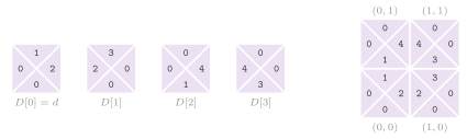
The square tiling. In BOUNDED TILING (the DOMINO LIMITATO of the
book), the \(n \times n\) squares of a board are to be covered with copies
of \(m\) oriented tiles, each split by its diagonals into four colored
quarters, never rotated, with the tile \(d = D[ 0 ]\) in the corner \(( 0 , 0
)\) and touching sides of the same color (Figure 20.2).
A Tile holds the colors of its four sides, and the square \(( i , j )\) is
the column \(i\) and the row \(j\) from the bottom left; a covering is a
Tiling, a matrix whose entry \(( i , j )\) is the index in \(D\) of the tile
of that square. The function legalTiling() is the certificate, in \(O( n^2 )\). The enumeration squareTiling() fills the squares by rows from
the bottom, and places a tile only if it fits its left and lower
neighbours, which prunes the enumeration of the \(m^{n^2 - 1}\) coverings at
the first wrong side (Algorithm 20.6).
Algorithm 20.6. The certificate and the enumeration of BOUNDED TILING (Montresor 2025, chapter 18).
We remark that the pruning of the enumerations usually changes the time in practice, but never the bound of Table 20.1: there are instances (e.g., those with no solution and no early failure) on which the tree is visited in full.
20.4 Reductions and NP-completeness¶
A polynomial reduction of \(A\) to \(B\) is a function \(f\), computable in polynomial time, such that
written \(A \propto B\) (Montresor 2025, §18.4).
Lemma 20.2. The relation \(\propto\) is transitive, and \(A \propto B\) with \(B \in \mathrm{P}\) gives \(A \in \mathrm{P}\).
Proof. An algorithm of polynomial time writes an output of polynomial size, and therefore \(\lvert f( x ) \rvert \le q( \lvert x \rvert )\) for a polynomial \(q\). Hence a polynomial algorithm for \(B\) run on \(f( x )\), and a second reduction applied to \(f( x )\), take time polynomial in \(\lvert x \rvert\), since a polynomial of a polynomial is a polynomial. \(\square\)
A problem is NP-hard if each problem of NP reduces to it, and NP-complete if it is also in NP; one NP-complete problem in P would give \(\mathrm{P} = \mathrm{NP}\), and, by Lemma 20.2, a problem of NP to which a known NP-complete problem reduces is NP-complete in its turn.
Theorem 20.1 (Cook; Levin). SATISFIABILITY is NP-complete.
We refer to Cook 1971 and Levin
1973 for the proof, which writes, for a
nondeterministic algorithm of polynomial time and an input \(x\), a formula
of polynomial size whose variables describe the contents of the memory at
each step and whose clauses force each step to follow from the one before
it; the formula is satisfiable if and only if a sequence of choices leads
to success. The book starts the chain from BOUNDED TILING instead, whose
rows of tiles can encode the successive configurations of a computation in
the same way (the tiles of Wang 1961),
and reduces it to the other problems, as Karp
1972 did from SATISFIABILITY. Altogether, the functions
of Reductions.h, and those of Problems.h that delegate to one another,
realize the chain of Table 20.2, each in the
time needed to write its output.
Table 20.2. The reductions realized in
ADS/complexity (Montresor 2025, §18.5 and
§18.7).
| From | To | Where | Function |
|---|---|---|---|
| BOUNDED TILING | CLIQUE | Theorem 18.2 | dominoToClique() |
| BOUNDED TILING | SATISFIABILITY | Theorem 18.3 | dominoToSat() |
| BOUNDED TILING | 0-1 INTEGER PROGRAMMING | Theorem 18.4 | dominoToLp01() |
| CLIQUE | INDEPENDENT SET | Theorem 18.5 | complement() |
| INDEPENDENT SET | VERTEX COVER | exercise 18.11 | the complement of the set, \(k' = n - k\) |
| HAMILTONIAN CIRCUIT | TRAVELING SALESMAN | Theorem 18.6 | hamiltonToTsp() |
| PARTITION | MULTIPROCESSOR SCHEDULING, SUBSET SUM, KNAPSACK | Theorems 18.7 to 18.9 | halfSum() |
| HAMILTONIAN CIRCUIT | DIRECTED HAMILTONIAN CIRCUIT | exercise 18.12 | both the orientations of each edge |
| DIRECTED HAMILTONIAN CIRCUIT | DIRECTED HAMILTONIAN PATH | exercise 18.13 | cycleToPath() |
| DIRECTED HAMILTONIAN CIRCUIT | HAMILTONIAN PATH | exercise 18.14 | cycleToChain() |
| DIRECTED HAMILTONIAN PATH | LONGEST PATH | exercise 18.15 | \(k = n - 1\) |
| HAMILTONIAN PATH | DEGREE-CONSTRAINED SPANNING TREE | exercise 18.16 | \(k = 2\) |
| 3-DIMENSIONAL MATCHING | EXACT COVER BY 3-SETS | chapter 18 | threeDimensionalMatching() |
Each reduction rests on a correspondence between the certificates of the
two problems, which we now state for the reductions from the tiling, the
others being (somewhat) simpler. In all of them, the node, or the variable, of the tile \(h\) in the
square \(( i , j )\) is \(u_{hij}\), at the place \(( h n + i ) n + j\) given by
tileVar().
Lemma 20.3. In the graph of
dominoToClique(), with \(m n^2\) nodes, the cliques of \(n^2\) nodes are the
legal coverings when \(n \ge 2\); hence BOUNDED TILING \(\propto\) CLIQUE, in
time \(\Theta( m^2 n^4 )\).
Proof. The graph joins \(u_{hij}\) to all the nodes of the squares not adjacent to \(( i , j )\), and to the nodes of the adjacent squares whose tile fits next to \(h\), and it leaves isolated the nodes of \(( 0 , 0 )\) but \(u_{000}\). Two nodes of one square are never joined, and therefore a clique of \(n^2\) nodes takes one tile per square, the tile \(d\) in \(( 0 , 0 )\); two of its tiles in adjacent squares are joined, i.e., they fit, and the clique is a legal covering. Conversely, the nodes of a legal covering are pairwise joined. Finally, the adjacency matrix has \(( m n^2 )^2\) entries. For \(n = 1\) an isolated node \(u_{h00}\), \(h \ne 0\), is a clique of one node too, but there both answers are YES (the tile \(d\) alone covers the board), and the reduction still satisfies (20.3). \(\square\)
The function dominoToSat() writes the same conditions as clauses on the variables
\(u_{hij}\), true if the tile \(h\) is in \(( i , j )\). They are the unit clause
\(u_{000}\), at least one tile and at most one tile in each square, and,
for each pair of adjacent squares and each pair of tiles that do not fit
there side by side, the clause that forbids both. The function dominoToLp01() writes
them as linear constraints: \(x_{000} = 1\), one tile per square (each
equation as two inequalities), and \(x_{hij}\) plus the tiles that do not fit
next to it in a neighbouring square at most 1; the example of the text
writes one inequality per pair, which is the same, since a square holds one
tile (Algorithm 20.7).
Algorithm 20.7. The reductions of BOUNDED TILING to CLIQUE, to SATISFIABILITY and to 0-1 INTEGER PROGRAMMING (Theorems 18.2 to 18.4 of Montresor 2025).
The other reductions of the chain are simpler
(Algorithm 20.8). The first, complement(), gives the
complement graph, which has the edge \([ u , v ]\), \(u \ne v\), exactly when
\(G\) does not, and hamiltonToTsp() gives the distance 1 on the edges of
\(G\) and 2 elsewhere, with \(k = n\). The bound of halfSum() is half the sum
of the numbers, or \(-1\) if the sum is odd, and the three numerical
problems take the numbers themselves as the times of the programs on two
processors with the deadline \(s / 2\), as the elements of SUBSET SUM, and
as the profits and the volumes of KNAPSACK with the capacity and the
target \(s / 2\). The function cycleToPath() splits the node 0 into a new node \(n\),
which takes the edges out of 0, and the node 0, which keeps the edges into
it. Finally, cycleToChain() makes each node \(v\) of the graph of
cycleToPath() a chain \(v_{in} - v_{mid} - v_{out}\), each edge \(( u , v
)\) an edge \([ u_{out} , v_{in} ]\), and adds a pendant node joined to
\(n_{in}\) and one joined to \(0_{out}\), \(3 ( n + 1 ) + 2\) nodes in all. Both
drop the loops of \(G\), as the problems of Problems.h ignore them.
Algorithm 20.8. The reductions of CLIQUE to INDEPENDENT SET, of HAMILTONIAN CIRCUIT to TRAVELING SALESMAN, of PARTITION to the numerical problems, and of the directed Hamiltonian circuit to the paths.
Lemma 20.4. Each function of Algorithm 20.8, and the complement of the set with \(k' = n - k\), satisfies (20.3) for the pair of problems of its row of Table 20.2, in time linear in the size of its output.
Proof. A set \(S\) is independent in \(G\) if and only if any two of its
nodes are joined in the complement graph, i.e., \(S\) is a clique there.
Also, \(S\) is independent if and only if \(V \setminus S\) covers the edges,
since an edge left uncovered by \(V \setminus S\) has both its ends in \(S\);
hence \(G\) has an independent set of \(k\) nodes if and only if it has a
cover of \(n - k\) nodes. With the distances of hamiltonToTsp(), a tour
has \(n\) edges of length at least 1, and its length is at most \(n\) if and
only if all its edges are edges of \(G\), i.e., the tour is a Hamiltonian
circuit of \(G\). If the sum \(s\) of the numbers is odd, no subset has the sum
\(s / 2\), and the bound \(-1\) has no YES in any of the three problems, whose
numbers are not negative. Otherwise, a subset of sum \(s / 2\) leaves the
other half to the second processor, or out of the knapsack, and
conversely a schedule within \(s / 2\) on two processors, a subset of sum
\(s / 2\) or a knapsack of volume at most \(s / 2\) and profit at least \(s / 2\)
splits the numbers into two halves of equal sum. For cycleToPath(), a
Hamiltonian cycle of \(G\) read from the node 0, \(0 , v_1 , \ldots ,
v_{n-1} , 0\), becomes the path \(n , v_1 , \ldots , v_{n-1} , 0\), whose
first edge is an edge out of 0 moved to \(n\), and conversely. For
cycleToChain(), a directed Hamiltonian path \(n = w_0 , w_1 , \ldots ,
w_n = 0\) gives the path that starts at the pendant node of \(n_{in}\), runs
along each chain \(w_{i,in} , w_{i,mid} , w_{i,out}\), passes from
\(w_{i,out}\) to \(w_{i+1,in}\) by the edge of \(( w_i , w_{i+1} )\), and ends
at the pendant node of \(0_{out}\). Conversely, in a Hamiltonian path of the
unoriented graph the two pendant nodes, of degree 1, are the two ends,
and each node \(v_{mid}\), of degree 2 and not an end, is passed between
\(v_{in}\) and \(v_{out}\). Hence the path, from the pendant node of \(n_{in}\),
runs along the chain of \(n\) from \(n_{in}\) to \(n_{out}\); from a node
\(u_{out}\) it can only go to a node \(v_{in}\) with \(( u , v )\) an edge of
the graph of cycleToPath() (or to the final pendant node, if \(u = 0\)),
and from \(v_{in}\) along the chain of \(v\) to \(v_{out}\). By induction the
chains are crossed in the order of a directed Hamiltonian path from \(n\)
to 0. Each function writes each entry of its output a constant number of
times. \(\square\)
The same tool proves lower bounds within P. Sorting reduces to the convex
hull (sortToHull(), Algorithm 20.9), which
maps each number \(a_i\) to the point \(( a_i , a_i^2 )\) of a parabola
(Montresor 2025, §18.5). Note that
the squares of the numbers must fit in a long, which is a precondition.
Algorithm 20.9. The reduction of sorting to the convex hull.
Lemma 20.5. The distinct points \(( a_i , a_i^2 )\) are all vertices of their convex hull, and its boundary in counterclockwise order from the leftmost vertex lists them by increasing \(a_i\). Hence an algorithm that computes the convex hull of \(n\) points with \(o( n \log n )\) comparisons would sort \(n\) numbers with \(o( n \log n )\) comparisons, and the convex hull costs \(\Omega( n \log n )\) comparisons in the worst case.
Proof. For a point \(( b , b^2 )\) of the set, the line \(y = 2 b x - b^2\) leaves all the other points \(( a , a^2 )\) strictly above it, since \(a^2 - 2 b a + b^2 = ( a - b )^2 > 0\); hence \(( b , b^2 )\) is the only point of the set that minimizes \(y - 2 b x\), i.e., a vertex of the hull. The points below the segment that joins the leftmost and the rightmost point are the lower chain of the hull, which a counterclockwise traversal visits from the leftmost to the rightmost vertex by increasing abscissa, and no point lies above that segment, by the convexity of \(x^2\); thus the traversal from the leftmost vertex is the sorted order. Equal numbers give the same point, and the order of the distinct values, with their multiplicities counted in \(O( n )\) by a scan, is the sorted sequence. The map and the reading of the hull cost \(O( n )\), and the lower bound \(\Omega( n \log n )\) of the sorting by comparisons applies. \(\square\)
20.5 Polynomial cases¶
The square tiling is NP-complete, while the tiling of a strip \(1 \times n\) is in P (Montresor 2025, §18.5). A strip is a walk of \(n - 1\) edges from \(d\) in the graph \(H\) whose nodes are the \(m\) tiles and whose edges \(( d_u , d_v )\) join a tile to those that fit on its right.
Lemma 20.6 (the linear tiling). A strip of \(n\) tiles from \(d\) exists if and only if
\(L( d )\) being the number of the edges of the longest path from \(d\).
The function linearTiling() decides (20.4) in \(O( m^2 )\) time, whatever \(n\) is.
Proof. A walk may go round a reachable cycle as many times as it needs, and so has any length; without a reachable cycle, each walk from \(d\) is a path, and its length is at most \(L( d )\). One visit in depth of \(H\) from \(d\) finds a reachable cycle as a back edge, i.e., an edge to a node still open, and computes \(L\) in the postvisit, since without cycles the longest path from \(u\) is one edge plus the longest from a successor. The visit examines the \(m^2\) pairs of tiles of the implicit matrix of \(H\) once each. \(\square\)
Note that \(n\) enters the input with \(\log n\) bits, and an enumeration of the strips would take time exponential in it; the visit, instead, does not depend on \(n\) at all (Algorithm 20.10).
Algorithm 20.10. The linear tiling by a visit in depth of the graph of the tiles.
In its conclusion, Montresor 2025
pairs several NP-complete problems with a polynomial one that differs from
it in a detail, and EasyCases.h realizes the polynomial halves that the
other areas do not (Table 20.3).
Table 20.3. The polynomial halves of the pairs of table 19.1 of the book, and where the library realizes them.
| NP-complete | Polynomial | Where |
|---|---|---|
| SATISFIABILITY, three literals per clause | two literals per clause | twoSat() |
| 3-COLORABILITY | 2-COLORABILITY | twoColoring() |
| 3-DIMENSIONAL MATCHING | 2-DIMENSIONAL MATCHING | bipartiteMatching() |
| CLIQUE | CLIQUE on an interval graph | intervalClique() |
| BOUNDED TILING | the linear tiling | linearTiling() of Domino.h |
| HAMILTONIAN CIRCUIT | the Eulerian cycle | eulerianCycle() of EulerianCycle.h |
| KNAPSACK | the fractional knapsack | fractionalKnapsack() (§13.11) |
| DEGREE-CONSTRAINED SPANNING TREE | the minimum spanning tree | kruskal() of MinimumSpanningTree.h |
| LONGEST PATH | the shortest path | shortestPaths() of ShortestPaths.h |
Theorem 20.2 (Aspvall, Plass and Tarjan). A formula of clauses of at most two literals is satisfiable if and only if no variable \(v\) lies in the strongly connected component of \(\neg v\) in the graph of the implications, which has the edges \(( \neg a , b )\) and \(( \neg b , a )\) for each clause \(a \vee b\); the assignment that makes \(v\) true when the component of \(v\) comes after that of \(\neg v\) in a topological order of the components satisfies the formula.
Proof. A path of implications from \(v\) to \(\neg v\) and one back would force \(v\) to be both true and false. Conversely, write \(\kappa( a )\) for the place of the component of the literal \(a\) in the topological order, so that an edge \(( a , b )\) gives \(\kappa( a ) \le \kappa( b )\). Suppose that the assignment of the statement sets a literal \(a\) true and a successor \(b\) of it false, i.e., \(\kappa( \neg a ) < \kappa( a )\) and \(\kappa( b ) < \kappa( \neg b )\). Since the graph is symmetric under negation (it has \(( \neg b , \neg a )\) whenever it has \(( a , b )\)), one has \(\kappa( \neg a ) < \kappa( a ) \le \kappa( b ) < \kappa( \neg b ) \le \kappa( \neg a )\), which is impossible. A clause \(a \vee b\) made false would give such a pair, the edge \(( \neg a , b )\) from a true literal to a false one (Aspvall, Plass and Tarjan 1979). \(\square\)
The function twoSat() takes a clause of one literal \(a\) as \(a \vee a\), builds the
graph of the \(2 n\) literals (the literal \(\pm( v + 1 )\) at the node \(2 v\)
or \(2 v + 1\), by literalNode()) with each implication once. Then it ranks
each strongly connected component by its first node in the order of
decreasing finish time of the visit in depth of topsort(), which is a
topological order of the components by
Lemma 20.7 below
(Algorithm 20.11). All this takes \(O( n + m
)\) time for \(m\) clauses (up to the logarithmic factor of the set that
removes the repeated implications).
Algorithm 20.11. The polynomial halves: 2-SATISFIABILITY, 2-COLORABILITY, the bipartite matching, and the cliques of an interval graph.
Similarly, a graph is 2-colorable if and only if it has no odd cycle,
which the visit in breadth of twoColoring() finds as an edge between two
nodes of the same color, in \(O( n^2 )\) on the adjacency matrix (the
diagonal ignored, as by coloring()). A bipartite matching is a maximum
flow with unit capacities from a source to the left nodes, along the
edges, to a sink (bipartiteMatching(), by the reduction of section 15.2
of the book). On intervals of the line, finally, a set that meets pairwise
has a common point, and the largest clique of the graph of the intervals
\([ a , b )\) built by intervalGraph() is counted by a sweep of the sorted
ends in \(O( n \log n )\) (intervalClique(), the right ends before the left
ones at equal abscissa).
Lemma 20.7. (i) If the components \(C\)
and \(C'\) of a graph are joined by an edge from \(C\) to \(C'\), the node of \(C\)
that finishes last in a visit in depth finishes after each node of \(C'\);
hence ranking the components by their first node in the order of
decreasing finish time is a topological order of the components. (ii)
twoColoring() returns a coloring with no edge between two nodes of the
same color if the graph has no odd cycle, and nil otherwise. (iii)
intervalClique() returns the largest number of intervals through one
point, which is the size of the largest clique of the graph of
intervalGraph(); an empty interval meets no other one.
Proof. (i) Let \(x\) be the first node of \(C \cup C'\) that the visit discovers. If \(x \in C\), all the nodes of \(C \cup C'\) are still new and reachable from \(x\), and hence they finish before \(x\). If \(x \in C'\), no node of \(C\) is reachable from \(C'\) (otherwise \(C\) and \(C'\) would be one component), and all the nodes of \(C'\) finish before the visit discovers a node of \(C\). In both cases a node of \(C\) finishes after all the nodes of \(C'\), and so the first node of \(C\) in the decreasing order precedes those of \(C'\). (ii) In the visit in breadth from a root \(r\), the color of a node is the parity of its distance from \(r\), and the distances of two adjacent nodes differ by at most 1. Hence an edge between two nodes of the same color joins two nodes at the same distance \(d\), and the two paths from \(r\) in the tree of the visit, with that edge, form a closed walk of \(2 d + 1\) edges, which contains an odd cycle; a graph with an odd cycle has no coloring with 2 colors, since the colors would alternate along the cycle. If the visit returns, each edge has been examined from both its ends with different colors. (iii) Two intervals \([ a , b )\) and \([ a' , b' )\) meet if and only if \(a < b'\) and \(a' < b\). For a set of intervals that meet pairwise, the largest left end \(a^*\) is below each right end, and hence belongs to all of them (the property of Helly in one dimension); thus the largest clique is the largest number of intervals through one point, and conversely the intervals through one point meet pairwise. In the sweep, after the events of the abscissae up to \(x\), the right ends at \(x\) first, \(c\) is the number of the intervals \([ a , b )\) with \(a \le x < b\), i.e., through \(x\); the values of \(c\) between two such moments are not larger than one of them, and an empty interval \([ a , a )\) adds \(-1\) before \(+1\) at \(a\). \(\square\)
20.6 Pseudopolynomial algorithms¶
We now turn to the strategies for the problems that are NP-hard. A problem of optimization requires, for an instance \(x\), a feasible solution of least cost (or of largest value) among the set \(F( x )\) of the feasible ones; \(x^*\) is an optimal solution and \(\mathit{OPT} = c( x^* )\) its cost. When the decision version is NP-complete, no algorithm is known that finds \(x^*\) in polynomial time on each instance, and each strategy gives up something. An algorithm is pseudopolynomial if its time is bounded by a polynomial in the size \(d\) of the instance and in its largest integer \(\#\) (Montresor 2025, §19.1); since \(\#\) may be exponential in \(d\), such an algorithm is polynomial only on the instances whose numbers are "small". For SUBSET SUM, with \(M[ i ][ j ]\) true if some of the first \(i\) elements sum to \(j\),
since a subset of the first \(i\) elements either avoids the \(i\)-th or takes
it once. The function subsetSumDP() of Pseudopolynomial.h fills (20.5) in \(O( n k )\)
time with one row of \(k + 1\) bits, written from the right, so that \(M[ j -
A_i ]\) is still the value of the row before
(Algorithm 20.12). The row is a vector of
Bits, which may be std::vector< bool > (the default),
boost::dynamic_bitset or the BitVector of the library, with the same
cells written. If a pointer rows is given, the function appends there the
row after each element. The function subsetSumSet() keeps all the rows, and reads a
subset backwards (an element is needed when the row above does not have
the sum), in \(O( n k )\) time and space; partitionDP() (exercise 19.1) is
the same with half the sum.
Algorithm 20.12. SUBSET SUM and PARTITION by dynamic programming (Montresor 2025, §19.1 and exercise 19.1).
Lemma 20.8. After the \(i\)-th element
\(a = A_i\) of line 4, \(M[ j ] = M[ i ][ j ]\) of (20.5) for \(0 \le j \le k\);
hence subsetSumDP() decides SUBSET SUM in \(O( n k )\) time and \(k + 1\)
bits.
Proof. Before the first element, \(M[ j ]\) is true only for \(j = 0\), the sum of the empty subset. Let the claim hold after the element \(i - 1\). In the pass of line 4 for \(a = A_i\), the entry \(j\) is written after the entries above it and before those below it; hence, when \(M[ j ]\) is written, \(M[ j - a ]\), with \(j - a \le j\), still holds \(M[ i - 1 ][ j - a ]\) (for \(a = 0\) the two are the same entry, and the or leaves it as it was). The entry \(j\) thus becomes \(M[ i - 1 ][ j ]\) or \(M[ i - 1 ][ j - a ]\), which is (20.5), while the entries \(j < a\), not written, keep \(M[ i - 1 ][ j ] = M[ i ][ j ]\). Finally, (20.5) is correct, since a subset of the first \(i\) elements either avoids the \(i\)-th or takes it once. \(\square\)
With more parts, the same idea gives the other dynamic programmings of
the header (Algorithm 20.13). In bottino()
(exercise 19.5), three thieves share jewels of prices \(P[ i ]\) so that
each takes a third of the value \(m\). There \(S[ i ][ j ][ h ]\) records
whether the first \(i\) jewels give \(j\) to the first thief and \(h\) to the
second, the third taking what is left; since the prices are not negative \(j\) and
\(h\) range in \([ 0 , m / 3 ]\), i.e., \(O( n m^2 )\) entries. In
schedulingDP() (exercise 19.2), the vectors of the loads of the \(m\)
processors reachable with the first \(i\) programs, each load at most \(d\),
are at most \(( d + 1 )^m\) after each program, and the time is \(O( n ( d + 1
)^m )\), pseudopolynomial for \(m\) fixed.
Algorithm 20.13. The loot of the three thieves, and MULTIPROCESSOR SCHEDULING by the vectors of the loads.
A problem is strongly NP-complete if it stays NP-complete on the instances with \(\#\) bounded by a polynomial in \(d\) (CLIQUE, whose numbers are bounded by \(n\), TRAVELING SALESMAN, 3-PARTITION), and weakly otherwise (SUBSET SUM, PARTITION, KNAPSACK); cf. Garey and Johnson 1978.
Theorem 20.3. A strongly NP-complete problem has no pseudopolynomial algorithm unless \(\mathrm{P} = \mathrm{NP}\).
Proof. On the instances with \(\# \le q( d )\), \(q\) a polynomial, the time of a pseudopolynomial algorithm is a polynomial in \(d\) and \(q( d )\), i.e., in \(d\); such an algorithm would solve in polynomial time a restriction that is NP-complete. \(\square\)
When a program may be interrupted and resumed on another processor, the scheduling becomes easy. No schedule is shorter than
since each program runs for its time and the \(m\) processors do at most \(m
d\) work, and the rule of McNaughton 1959
(mcNaughton(), exercise 19.3) reaches (20.6) by filling the processors
one after the other up to \(d\), in \(O( n + m )\) time
(Algorithm 20.14).
Lemma 20.9. The schedule of mcNaughton()
runs each program for its time within \([ 0 , d ]\), and never on two
processors at once; hence it is optimal, and realTimeScheduling()
succeeds if and only if \(C_i \le T_i\) for each \(i\) and \(\sum_i C_i / T_i
\le m\).
Proof. A program split between the processors \(q\) and \(q + 1\) runs on
\(q\) from some time \(s\) to \(d\), and on \(q + 1\) from 0 to \(t_i - ( d - s )\);
since \(t_i \le d\), one has \(t_i - ( d - s ) \le s\), and the two pieces do
not overlap in time. Also, the total work \(\sum_i t_i \le m d\) fits in the \(m\)
processors, and the loop of line 5 never runs out of processors with work
left. The length \(d\) is the lower bound (20.6), and hence optimal. For
realTimeScheduling(), \(d \le 1\) if and only if \(\max_i C_i / T_i \le 1\)
and \(\sum_i C_i / T_i \le m\). When \(d > 1\), no schedule of a period
exists, again by (20.6). \(\square\)
With \(t_i = C_i / T_i\) and \(d = 1\), the same rule schedules a period of
the periodic tasks of REAL-TIME SCHEDULING without a priority rule
(realTimeScheduling(), exercise 19.4), the task \(i\) running for the
fraction \(C_i / T_i\) of each period, which succeeds if and only if \(C_i \le
T_i\) for each \(i\) and \(\sum_i C_i / T_i \le m\). Schedules are lists of
Pieces, each the program and the interval \([ \mathit{start} ,
\mathit{end} )\) in which it runs, and the contracts check them as a
postcondition.
Algorithm 20.14. The rule of McNaughton, and REAL-TIME SCHEDULING (Montresor 2025, exercises 19.3 and 19.4).
20.7 Approximation algorithms¶
An algorithm is an approximation with relative error \(e\) if it gives a feasible \(x'\) with
on each instance, and an approximation scheme if it takes \(\epsilon >
0\) in input and satisfies (20.7) with \(e = \epsilon\) in a time polynomial
in \(d\) for each fixed \(\epsilon\) (fully polynomial if also in \(1 /
\epsilon\)) (Montresor 2025, §19.2).
All the guarantees of Approximation.h rest on a lower bound of
\(\mathit{OPT}\) that the algorithm can compare with its own cost
(Table 20.4).
Table 20.4. The approximations of
Approximation.h (Montresor 2025, §19.2 and exercises 19.6 and
19.8); \(N\) and \(N^*\) are the boxes
used and the fewest possible.
| Problem | Function | Guarantee | Time |
|---|---|---|---|
| BIN PACKING | firstFit() |
\(N < 2 N^*\) | \(O( n^2 )\) |
| TRAVELING SALESMAN, triangular | deltaTsp() |
\(c( x' ) \le 2 \, \mathit{OPT}\) | \(O( n^2 \log n )\) |
| SUBSET SUM | apSubsetSum() |
\(e < 1 / ( h + 1 )\) | \(O( h n^{h+1} )\) |
| VERTEX COVER | vertexCoverApprox() |
\(\lvert S \rvert \le 2 \, \mathit{OPT}\) | \(O( n^2 )\) |
| KNAPSACK | knapsackApprox() |
\(c( x' ) \ge ( 1 - \epsilon ) \mathit{OPT}\) | \(O( n^3 / \epsilon )\) |
Bin packing. The function firstFit() puts each object of volume in \([ 0 , k ]\)
in the first box with room for it, the objects in the order given (ff) or
by decreasing volume (ffd), and opens a new box when none has room
(Algorithm 20.15).
Algorithm 20.15. The first fit, and its decreasing variant, for BIN PACKING.
Lemma 20.10. If some object has a positive volume, the first fit uses \(N < 2 N^*\) boxes.
Proof. No two boxes have contents that sum to at most \(k\), since the objects of the later one would have fitted in the earlier one. If \(N \ge 2\), summing the contents of the \(N\) pairs of consecutive boxes (the last with the first) counts each box twice, and twice the total volume \(V\) exceeds \(N k\); since \(N^* \ge V / k\), one has \(N < 2 V / k \le 2 N^*\). If \(N = 1\), then \(N^* = 1\). \(\square\)
In practice, the decreasing order of ffd usually helps, and it improves the constant, to \(11 / 9\) asymptotically (Johnson et al. 1974). Since a box is found by a scan, the time is \(O( n N )\), i.e., \(O( n^2 )\) in the worst case.
The triangular salesman. The function deltaTsp() builds a minimum spanning tree
\(T\) of the complete graph of the symmetric distances (by kruskal() on
the \(n ( n - 1 ) / 2\) edges, whence the time \(O( n^2 \log n )\)), and
returns the cities in the preorder of \(T\) from 0, the children by
increasing name (Algorithm 20.16;
Rosenkrantz, Stearns and Lewis 1977).
The function tourCost() gives the cost of a circuit.
Lemma 20.11. If the distances satisfy the
triangle inequality, the circuit of deltaTsp() costs at most \(2 \,
\mathit{OPT}\).
Proof. The tree \(T\) weighs no more than any circuit, which is a spanning path plus an edge of nonnegative cost, and the walk that goes twice along each edge of \(T\) costs \(2 w( T ) \le 2 \, \mathit{OPT}\). Then the preorder visits the cities in the order of their first visit by the walk, and each shortcut over the cities already visited costs no more than the stretch of the walk that it replaces, by the triangle inequality. \(\square\)
The bound is reached, up to a vanishing term, by the two concentric polygons of figure 19.3 of the book. We remark that the triangle inequality is checked by an audit in \(O( n^3 )\), with a relative tolerance for the floating point. Without it there is no constant at all, as follows.
Theorem 20.4. For no constant \(s \ge 1\) does TRAVELING SALESMAN have a polynomial algorithm with \(c( x' ) \le s \, \mathit{OPT}\), unless \(\mathrm{P} = \mathrm{NP}\).
Proof. With the distances of tspGap(), 1 on the edges of \(G\) and \(s n\)
elsewhere, a Hamiltonian circuit of \(G\) is a tour of cost \(n\), while any
other tour costs more than \(s n\); an algorithm within \(s\) would therefore
return a tour of cost at most \(s n\) if and only if \(G\) has a Hamiltonian
circuit, and decide HAMILTONIAN CIRCUIT in polynomial time. \(\square\)
Algorithm 20.16. The salesman with the triangle inequality, and the distances of Theorem 19.2 of the book.
Subset sum. For the optimization version of SUBSET SUM (the largest
sum at most \(k\)), apSubsetSum() tries each set of at most \(h\) elements,
in the order of the text (by size, then lexicographically on the elements
in decreasing order), and completes it greedily on the elements in
decreasing order (Algorithm 20.17).
Lemma 20.12. Let \(z^* \le k\) be the
optimum. The sum \(z\) found by apSubsetSum() is either \(z^*\), or
the time is \(O( h n^{h+1} )\).
Proof. Let \(S^*\) be optimal. If \(\lvert S^* \rvert \le h\), the algorithm tries \(S^*\) itself. Otherwise it tries the \(h\) largest elements of \(S^*\), and the greedy completion either takes all of \(S^*\) or leaves out an element \(a\) of \(S^*\), not larger than those \(h\), with \(z + a > k \ge z^*\). Since \(( h + 1 ) a \le z^*\), one has \(z > z^* - a \ge z^* ( 1 - 1 / ( h + 1 ) )\). As for the time, the \(O( n^h )\) sets of at most \(h\) elements are each built in \(O( h )\) and completed in \(O( n )\). \(\square\)
Algorithm 20.17. The approximation of SUBSET SUM, the cover by the ends of a matching, and the approximation scheme of KNAPSACK.
Vertex cover. The function vertexCoverApprox() (exercise 19.6) takes both the
ends of each edge \([ u , v ]\), \(u < v\), whose ends are both out of the
cover so far.
Lemma 20.13. vertexCoverApprox()
returns a vertex cover \(S\) with \(\lvert S \rvert \le 2 \, \mathit{OPT}\),
in \(O( n^2 )\) time on the adjacency matrix.
Proof. An edge whose ends are not both out of \(S\) when it is examined has an end in \(S\), and the edges examined later only add nodes; an edge examined with both ends out of \(S\) puts them in. Hence \(S\) is a cover. The edges that put their ends in \(S\) share no end, since each of them had both ends out of \(S\), i.e., they form a matching \(M\), and \(\lvert S \rvert = 2 \lvert M \rvert\). Any cover has an end of each edge of \(M\), and these ends are distinct; hence \(\mathit{OPT} \ge \lvert M \rvert\). The loop examines the \(n ( n - 1 ) / 2\) pairs \(u < v\). \(\square\)
Knapsack. The function knapsackApprox() (exercise 19.8) is the scheme of Ibarra
and Kim 1975: it keeps the objects that
fit by themselves, divides their profits by \(K = \max\{ 1 , \epsilon \, p_{\max}
/ n' \}\), \(n'\) being their number and \(p_{\max}\) their largest profit, and
rounds them down; then it finds, by dynamic programming, the least volume
\(V[ i ][ s ]\) of the first \(i\) objects of rounded profit \(s\), and returns
the set of largest rounded profit within the capacity.
Lemma 20.14. knapsackApprox() returns a
set of profit at least \(( 1 - \epsilon ) \, \mathit{OPT}\), in \(O( n^3 /
\epsilon )\) time.
Proof. Rounding a profit down to a multiple of \(K\) loses less than \(K\), and therefore less than \(n' K\) on any set, which is \(\epsilon \, p_{\max}\) if \(K > 1\) (and nothing if \(K = 1\), since the profits are integers). The set optimal for the rounded profits is thus within \(\epsilon \, p_{\max} \le \epsilon \, \mathit{OPT}\) of the optimum, since each of the objects kept fits alone. As for the time, the table has a column per rounded profit, at most \(n' \cdot n' / \epsilon\) of them, and a row per object. \(\square\)
20.8 Branch-and-bound¶
A branch-and-bound visits the tree of the partial solutions of the enumeration of chapter 19 (backtracking), and skips a subtree when a lower bound of the costs in it is not below the best cost found (Montresor 2025, §19.3).
Lemma 20.15 (the bound). If \(\mathit{lb}( S ) \le c( x )\) for each complete solution \(x\) that extends the partial solution \(S\), then skipping \(S\) when
loses no solution better than the best found so far, and the visit returns an optimum.
Proof. A solution \(x\) in the subtree of a skipped \(S\) has \(c( x ) \ge \mathit{lb}( S ) \ge \mathit{minCost}\), and the best found so far is at least as good. The solutions not skipped are all compared. \(\square\)
Note that the guarantee holds whatever the order of the visit and the bound, and the
time in the worst case stays that of the enumeration; what changes is the
number of the nodes in practice, which bbTsp(), littleTsp(),
maxWeightClique() and the knapsacks report in *generated, if given.
The salesman, depth first. The function bbTsp() chooses the cities of the circuit
one after the other from \(S[ 0 ] = 0\), in increasing order, depth first,
starting from the circuit start if one is given
(Algorithm 20.18). A child is generated for
each city not in \(S\), and visited only if its bound is below the best; a
complete circuit is the bound of its last node, i.e., its cost.
The function tspLowerBound() computes two bounds, chosen by TspBound. Let \(S = S[ 0 .. i ]\) be the path chosen, \(C_i\) its length and \(R\) the cities out of \(S\). We write \(A\) for the least distance from a city of \(R\) back to \(S[ 0 ]\), \(B\) the least
distance from \(S[ i ]\) to a city of \(R\), and \(D_h\), for \(h \in R\), the least
cost \(D[ p ][ h ] + D[ h ][ q ]\) of entering and leaving \(h\) over the
cities \(p \ne q\) different from \(h\).
Lemma 20.16. Both
with \(T_R\) a minimum spanning tree of \(R\) (the ceiling only on integer distances, and the second bound for symmetric distances), satisfy the hypothesis of Lemma 20.15.
Proof. A circuit that extends \(S\) goes on from \(S[ i ]\) through all the cities of \(R\) and back to \(S[ 0 ]\), with \(\lvert R \rvert + 1\) edges. Each city of \(R\) is entered once and left once, which costs at least \(D_h\); the sum of the \(D_h\) counts each edge of the rest of the circuit between two cities of \(R\) twice, and the first and the last edge once, which cost at least \(B\) and \(A\). Hence the rest costs at least half the sum, and the cost is an integer on integer distances. For the 1-tree, the rest is a path through the cities of \(R\), i.e., a spanning tree of \(R\), plus its first and last edge. \(\square\)
Our first bound is that of the text (TspBound::BOOK), which uses the
least distances into and out of each city over all the cities, as in its
example (\(\mathit{lb} = 18\) for \(S = 1 , 3\) of figure 19.5 of the book;
there the least distance \(A\) is taken from \(S[ 0 ]\), which is the same for
symmetric distances). We remark that two values of figure 19.6 of the
book do not follow from this formula (21 for \(1 , 2 , 3\) and for \(1 , 5\),
where it gives 19 and 20), and we found no rule that gives all the values
of the figure. With the formula and the circuit \(1 , 4 , 3 , 2 , 5\) of cost
21 to start from, the tree has 25 nodes instead of 23 (30 with no circuit
to start from), and it ends with the same circuit \(1 , 3 , 2 , 5 , 4\) of
cost 19 (we suspect a slip in the figure, although we cannot exclude another rule). The second bound is that of the
1-tree of Held and Karp 1971 (exercise
19.10), which replaces the sum by the weight of a minimum spanning tree of
the cities out of \(S\). Also, spanningTreeWeight() and oneTree() compute the
tree of a set of cities and the minimum 1-tree of a city (a minimum
spanning tree of the others plus the two least edges of that city), which
bounds the optimum from below, since each circuit is a 1-tree.
Algorithm 20.18. The salesman by branch-and-bound with the bound of the text or of the 1-tree (Montresor 2025, §19.3.1 and exercise 19.10).
The salesman, by the reduction of the matrix. The function littleTsp() (exercise
19.11, the algorithm of Little et al. 1963)
branches on including or excluding an edge, the entry 0 of the reduced
matrix whose exclusion raises the bound the most, visits the nodes by
least bound with a priority queue, and bounds a node by reducing the rows
and the columns of its matrix to a least entry 0
(Algorithm 20.19). Subtracting a constant
from a row or a column lowers the cost of each circuit by that constant,
since a circuit uses one entry of each row and one of each column. Hence the sum of the constants subtracted is a lower bound, and the entries 0
left are the edges that a circuit of that cost would use. Including an edge
\(( i , j )\) marks its row and its column as done and sets to \(\infty\) the
edge that would close a subcircuit, and excluding it sets \(M[ i ][ j ] =
\infty\).
Algorithm 20.19. The algorithm of Little, Murty, Sweeney and Karel (Montresor 2025, exercise 19.11).
Lemma 20.17. Let the circuits of a node \(x\) be those that contain the edges included in \(x\), the set \(I_x\), and no edge excluded in \(x\). Then \(c( H ) = \mathit{lb}_x + \sum_{e \in H \setminus I_x} M_x[ e ]\) for each circuit \(H\) of \(x\), with \(M_x \ge 0\) on the rows and the columns not done; hence \(\mathit{lb}_x \le c( H )\), and the first node of \(n\) edges extracted in line 5 is an optimal circuit.
Proof. At the root \(I_x\) is empty, \(\mathit{lb}_x = 0\) and \(M_x = D\) before the reduction. Subtracting \(\mu\) from a row not done lowers by \(\mu\) the entry of that row that each circuit of \(x\) uses outside \(I_x\) (there is exactly one, since no edge of \(I_x\) leaves that row), and adds \(\mu\) to \(\mathit{lb}_x\); the same holds for a column, and the minima subtracted leave the entries not negative. In the child \(y\), the edge \(( i , j )\) enters \(I_y\) with \(M_x[ i ][ j ] = 0\), so that the sum does not change, and the edge set to \(\infty\) would close a subcircuit, which no circuit of \(y\) contains. In the child \(z\) no circuit uses \(( i , j )\), and its entry does not appear in the sum. A child whose reduction fails has a row or a column with no finite entry, i.e., no circuit, and is dropped. The circuits of \(x\) are those of \(y\) and those of \(z\); hence the circuits of the root are, at any time, those of the nodes in \(Q\) and those already returned. A node of \(n\) edges has a single circuit, with \(H \setminus I_x = \emptyset\) and \(c( H ) = \mathit{lb}_x\). When such a node is extracted, each other circuit belongs to a node of \(Q\) whose bound is at least \(\mathit{lb}_x\), and therefore costs at least \(\mathit{lb}_x\). \(\square\)
Cliques and knapsacks. The function maxWeightClique() (exercise 19.9) extends a
set by the candidates adjacent to all of it, and prunes it when its weight
plus that of all its candidates is not above the best. The function knapsackBB()
(exercise 19.12) takes the objects by decreasing profit per volume, each
in and then out, and prunes a node when the fractional knapsack of the
objects left within the capacity left (§13.11)
does not beat the best. This is an upper bound of the best profit of the
objects left, since the fractional greedy is optimal for the relaxation
(Lemma 13.26). The function
knapsackBacktrack() is the
same visit with the objects in their order and the simple bound, the sum
of the profits still to decide. In turn, knapsackGreedy() is the heuristic that
takes the objects by decreasing profit per volume while they fit, which is
not optimal in general (Algorithm 20.20). The test beyond.knapsack-heuristics checks that the two visits find the
optimum of knapsack() and that the greedy finds no more.
Algorithm 20.20. The clique of largest weight, and KNAPSACK by branch-and-bound, by backtracking and by the greedy choice (Montresor 2025, exercises 19.9 and 19.12).
20.9 Heuristics¶
A heuristic gives a feasible solution with no guarantee on its cost
(Montresor 2025, §19.4); it is
judged by its time and by its results in practice, and the contracts of
Heuristics.h check that each result is feasible, not that it is "good".
Constructive heuristics. The constructive heuristics of the header are
greedy (Algorithm 20.21). The function greedyTsp()
keeps the lightest edges that leave each city with at most two of them
and close no cycle, as kruskal() does with an MFSET (chapter 11), and
so it ends with a Hamiltonian chain, which the edge of its two ends
closes; the sort of the \(n ( n - 1 ) / 2\) edges gives \(O( n^2 \log n )\).
The function greedySuperstring() (exercise 19.13) is the same greedy on the oriented
edges weighed by the overlaps of the strings (overlap( a , b ), the
longest suffix of \(a\) that is a prefix of \(b\)), which leaves oriented
paths, after dropping the strings contained in another. The function dsatur()
(exercise 19.19, Brélaz 1979) colors
first the node that sees the most colors among its neighbours, i.e., the
most constrained, with the least color not on its neighbours, in \(O( n^3 )\).
The function starAlignment() (exercise 19.18, after Gusfield
1993) aligns \(k\) strings against the
center, i.e., the string with the largest sum of the global scores against
the others. This takes \(O( k^2 \ell^2 )\) time for strings of length at most \(\ell\).
Algorithm 20.21. The greedy heuristics: the salesman, the superstring, the coloring by saturation degree and the star alignment (Montresor 2025, §19.4.1 and exercises 19.13, 19.18 and 19.19).
The bisection by buckets. The function minMaxGreedy() (the min-max-greedy of the
book) grows the two halves \(V_0\) and \(V_1\) of a bisection in turn, from a
node \(a\) in \(V_0\) and a node \(b\) in \(V_1\), each time with the node out of
them that has the fewest edges to the other half and, among those, the
most to its own (Algorithm 20.22). The
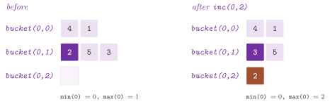
structure Buckets of exercise 19.17 keeps, for \(k = 0 , 1\), the nodes not
placed by the number \(h\) of their edges to \(V_k\). There bucket( k , h ) is a vector of nodes, whose size is dim( k , h ), each node knows its place in its two buckets, and
min( k ) and max( k ) are the least and the largest bucket not empty
(Figure 20.3). The function inc( k , u ) moves \(u\) to
the next bucket of side \(k\), by taking it out of its bucket (the last node
of the bucket fills its place) and appending it to the next one. In
turn, choose( k ) scans the least bucket of the other side for the node with the most
edges to \(V_k\), contains( u ) is true if \(u\) is still to be placed and
count( k , u ) gives its edges to \(V_k\). The size of the cut that
results, i.e., the number of edges between the two sides, is
cutSize( G , side ).
Lemma 20.18. insert(), remove() and
inc() cost \(O( 1 )\) amortized time, and minMaxGreedy() takes \(O( n^2 )\)
time on the adjacency matrix, \(O( n )\) choices of \(O( n )\) time each.
Proof. A node leaves a bucket in \(O( 1 )\) by its place, which the node
moved into it inherits (line 5 of remove() in
Algorithm 20.22). Furthermore, the bounds
\(\mathit{min}( k )\) and \(\mathit{max}( k )\) move by a scan (line 6)
only when a bucket empties. In
minMaxGreedy() all the nodes are inserted at the start, with the count
0, and the counts only grow. Hence \(\mathit{min}( k )\) never decreases, and
its scans move it forward at most \(n + 1\) places in all, while
\(\mathit{max}( k )\) grows by one at most per inc(), and its scans move
it down at most as many places as it grew, plus \(n + 1\). Each node placed updates the counts of its
neighbours, \(O( n )\) on the matrix, and each choice scans one bucket.
\(\square\)
Algorithm 20.22. The min-max-greedy for
the BISECTION, and the removal of a node from a Buckets (Montresor 2025,
§19.4.1 and exercise 19.17).
Local search. A local search starts from a solution \(\pi\) and moves
to a better solution of its neighbourhood \(I( \pi )\) while there is one. It ends at a local optimum, since the cost decreases strictly at each step
and the solutions are finitely many (Montresor 2025,
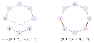
§19.4.2). For the salesman, the
neighbourhood \(I_2( \pi )\) of twoOpt() holds the circuits obtained by
removing two edges of \(\pi\) that do not touch, and reconnecting the two
paths in the only other way, i.e., by reversing the stretch between them
(Figure 20.4; Lin
1965), which gives
the pairs of edges less the \(n\) that touch. Since the change of cost of a move
depends only on the four edges that change, a step of the search, which takes the
best circuit of the neighbourhood, costs \(O( n^2 )\)
(Algorithm 20.23). The function twoOptMove( pi , i , j )
applies one move, reversing \(\pi[ i + 1 .. j ]\), and the costs of the
circuits visited go to *trace, if given.
Algorithm 20.23. The local search on \(I_2\), the size of \(I_k\), and the local search for PARTITION (Montresor 2025, §19.4.2 and exercises 19.15 and 19.16).
The function kOptNeighbours() (exercise 19.15) counts \(\lvert I_k( \pi ) \rvert\), the
circuits that share \(n - k\) edges with \(\pi\), by enumerating all the
circuits in \(O( n! )\), which checks (20.11) for \(k = 2\).
The function partitionLocalSearch() (exercise 19.16) does the same for PARTITION, with
the moves of one element and the swaps of two, each changing the
difference of the sums by twice the elements moved, the best move first,
in \(O( n^2 )\) per step. Arguably, the classical local search for the bisection,
whose moves swap two nodes, is that of Kernighan and Lin
1970; the library does not implement
it.
20.10 The fifteen puzzle¶
In the FIFTEEN PUZZLE (the GIOCO DEL QUINDICI of the book), \(n^2 - 1\) tiles
numbered from 1 lie on an \(n \times n\) grid with a hole, a move slides a
tile next to the hole into it, and the goal has the tiles in increasing
order and the hole last (Montresor 2025, §19.5).
A configuration is a Board, the tile of each square by rows, 0 the hole;
puzzleGoal() gives the goal and puzzleMoves() the configurations one
move away. The function solvePuzzle() is the branch-and-bound of the text, whose
nodes are the configurations and whose children are those one move away.
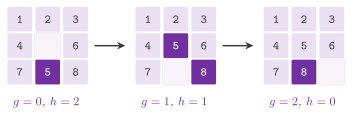
The cost of a node \(x\), \(g( x )\),
is the number of moves from the root, its lower bound \(h( x )\) is the sum
of the distances of the tiles from their places (manhattan()), and the
next node visited is the one of least \(f( x ) = g( x ) + h( x )\), by a
Fibonacci heap (Figure 20.5). The least
level met of each configuration is kept in a map, the parameter Map of
solvePuzzle() (std::map by default, or another map of the standard
library or of Boost, or a hash table of ADS), which changes the time but
not the nodes visited. This is the
algorithm A* of Hart, Nilsson and Raphael
1968 (Algorithm 20.24).
Algorithm 20.24. The fifteen puzzle by A*, by the visit in breadth and by backtracking, and the test of solvability (Montresor 2025, §19.5).
*Lemma 20.19 (A with a consistent bound).** If \(h\) is 0 at the goal and
then the first goal extracted from the queue is reached in the fewest moves, and each configuration is expanded at most once.
Proof. A move changes the place of one tile by one square, and so
changes manhattan() by at most 1, which is (20.12). Summing (20.12) along
a path to the goal shows that \(h\) never exceeds the moves left, and adding
\(g\) shows that \(f\) never decreases along a path. Let \(\delta( y )\) be the
fewest moves from the start to \(y\). We first show that a configuration \(y\)
is extracted (and not skipped as stale) only with \(g( y ) = \delta( y )\).
Otherwise, on a shortest path to \(y\) let \(z\) be the first configuration not
yet expanded with \(g( z ) = \delta( z )\); its predecessor was, and so \(z\)
is in the queue with \(g( z ) = \delta( z )\) and
\(f( z ) = \delta( z ) + h( z ) \le \delta( y ) + h( y ) < g( y ) + h( y )\)
by (20.12) along the path, and \(z\) would have been extracted before \(y\).
Hence each configuration \(y\) is expanded once: after it is expanded with
\(g( y ) = \delta( y )\), the map holds \(\delta( y )\), and any later entry
of \(y\) has \(g > \delta( y )\), since line 8 inserts \(y\) only with a level
smaller than the one stored, hence once with the level \(\delta( y )\); line
5 skips such an entry. Applied to the first
goal \(x\) extracted, \(g( x ) = \delta( x )\), i.e., it is reached in the
fewest moves. \(\square\)
We made the map a parameter of solvePuzzle(), std::map by default, and
the same search therefore runs with the maps of the standard library, of Boost or of
the library (e.g., FlatHashTable) and visits the same nodes; if a pointer
visited is given, the function counts there the nodes extracted. Beyond
the text, two searches work with any goal, e.g., the spiral one of
puzzleSpiralGoal() (Algorithm 20.24).
The function puzzleBFS() is the case \(h = 0\), the visit in breadth, whose first goal
reached is one of the fewest moves, and which examines many more
configurations than A*. In turn, puzzleDFS() is the backtracking that goes back
when a configuration is already on the current path or the moves exceed a
bound, and it finds a solution of at most that many moves if there is
one, not necessarily the shortest.
Lemma 20.20. Let \(I\) be the number of the inversions of the tiles read by rows, the hole left out, and \(r\) the row of the hole. A move keeps the parity of \(I\) when \(n\) is odd, and that of \(I + r\) when \(n\) is even; hence half of the configurations cannot reach the goal.
Proof. A move of the hole along a row leaves the order of the tiles unchanged. A move along a column moves one tile past the \(n - 1\) tiles between its two places in the order by rows, which changes \(I\) by an amount of the parity of \(n - 1\), and changes \(r\) by one. With \(n\) odd, \(n - 1\) is even; with \(n\) even, \(I\) and \(r\) change parity together. Exchanging two tiles changes the parity of \(I\) and leaves \(r\), and it therefore maps the configurations of one parity one to one onto those of the other. The two classes thus have the same size, and those of the parity other than that of the goal cannot reach it. \(\square\)
The function solvable() compares that parity with the one of the goal (Johnson and
Story 1879), which is also sufficient,
as they proved; solvePuzzle() calls it first, and answers nothing on a
configuration that cannot reach the goal, instead of exhausting the half
of the configurations that it can reach.
20.11 The interface¶
We collect here, header by header, the declarations of the namespace ADS
that a user calls in this chapter, without the contracts, the documentation
and the members that only the implementation uses; each block points to the
section that describes its functions, and the example at the end shows the
main structures at work. The program of the example compiles against the
headers as it stands, and its assertions hold.
// declarations of <ADS/complexity/Domino.h>
struct Tile
{
 int up , right , down , left;
 };
using Tiling = std::vector< std::vector< int > >;
bool legalTiling( const std::vector< Tile > & D , int n , const Tiling & T );
std::optional< Tiling > squareTiling( const std::vector< Tile > & D , int n );
bool linearTiling( const std::vector< Tile > & D , long n );
EasyCases.h (§20.5).
// declarations of <ADS/complexity/EasyCases.h>
int literalNode( int l );
std::optional< std::vector< bool > > twoSat( const Cnf & F , int n );
std::optional< std::vector< int > > twoColoring( const Adjacency & G );
std::vector< std::pair< int , int > >
bipartiteMatching( int p , int q ,
                   const std::vector< std::pair< int , int > > & E );
Adjacency intervalGraph( const std::vector< std::pair< long , long > > & I );
int intervalClique( const std::vector< std::pair< long , long > > & I );
// declarations of <ADS/complexity/Nondeterminism.h>
class Chooser
{
 public:
 int choice( int k );
 template< class A >
 bool run( A && alg , long * runs = nullptr );
 std::vector< int > choices( void ) const;
 };
Problems.h (§20.1).
// declarations of <ADS/complexity/Problems.h>
using Adjacency = std::vector< std::vector< bool > >;
using Clause = std::vector< int >;
using Cnf = std::vector< Clause >;
using Nodes = std::vector< int >;
bool cliqueCertificate( const Adjacency & G , const Nodes & S , int k );
std::optional< Nodes > clique( const Adjacency & G , int k );
std::optional< Nodes > independentSet( const Adjacency & G , int k );
std::optional< Nodes > vertexCover( const Adjacency & G , int k );
std::optional< std::vector< int > > coloring( const Adjacency & G , int k );
std::optional< Nodes > bisection( const Adjacency & G , int k );
template< class T >
bool tspCertificate( const std::vector< std::vector< T > > & D , T k ,
                     const Nodes & P );
template< class T >
std::optional< Nodes > tsp( const std::vector< std::vector< T > > & D , T k );
std::optional< Nodes > hamiltonianCircuit( const Adjacency & G );
std::optional< Nodes > hamiltonianCycle( const Adjacency & G );
std::optional< Nodes > hamiltonianPath( const Adjacency & G , int r = -1 ,
                                        int t = -1 );
std::optional< Nodes > hamiltonianChain( const Adjacency & G );
std::optional< Nodes > longestPath( const Adjacency & G , int r , int t ,
                                    int k );
int longestPathDag( const Adjacency & G , int r , int t );
std::optional< std::vector< std::pair< int , int > > >
boundedSpanningTree( const Adjacency & G , int k );
bool satCertificate( const Cnf & F , const std::vector< bool > & x );
std::optional< std::vector< bool > > satisfiable( const Cnf & F , int n );
std::optional< std::vector< int > >
lp01( const std::vector< std::vector< long > > & A ,
      const std::vector< long > & b , int n );
std::optional< Nodes > subsetSumExists( const std::vector< long > & A ,
                                        long k );
std::optional< Nodes > partition( const std::vector< long > & A );
std::optional< Nodes > knapsackDecision( const std::vector< long > & p ,
                                         const std::vector< long > & v ,
                                         long C ,
                                         long k );
std::optional< std::vector< int > >
multiprocessorScheduling( const std::vector< long > & t , int m , long d );
std::optional< Nodes >
exactCover3( const std::vector< std::array< int , 3 > > & Y , int m );
std::optional< Nodes >
threeDimensionalMatching( const std::vector< std::array< int , 3 > > & M ,
                          int q );
std::optional< std::vector< long > > bribes( std::vector< long > M ,
                                             const std::vector< bool > & ps );
// declarations of <ADS/complexity/Reductions.h>
int tileVar( int h , int i , int j , int n );
std::pair< Adjacency , int > dominoToClique( const std::vector< Tile > & D ,
                                            int n );
Cnf dominoToSat( const std::vector< Tile > & D , int n );
std::pair< std::vector< std::vector< long > > , std::vector< long > >
dominoToLp01( const std::vector< Tile > & D , int n );
Adjacency complement( const Adjacency & G );
std::vector< std::vector< long > > hamiltonToTsp( const Adjacency & G );
long halfSum( const std::vector< long > & A );
Adjacency cycleToPath( const Adjacency & G );
Adjacency cycleToChain( const Adjacency & G );
std::vector< Point > sortToHull( const std::vector< long > & a );
// declarations of <ADS/intractable/Approximation.h>
std::vector< int > firstFit( const std::vector< long > & A , long k ,
                             bool decreasing = false );
template< class T >
T tourCost( const std::vector< std::vector< T > > & D , const Nodes & S );
template< class T >
Nodes deltaTsp( const std::vector< std::vector< T > > & D );
std::vector< std::vector< long > > tspGap( const Adjacency & G , long s );
std::pair< long , Nodes > apSubsetSum( const std::vector< long > & A , long k ,
                                      int h );
std::pair< long , Nodes > knapsackApprox( const std::vector< long > & p ,
                                         const std::vector< long > & v ,
                                         long C ,
                                         double eps );
Nodes vertexCoverApprox( const Adjacency & G );
// declarations of <ADS/intractable/BranchAndBound.h>
enum class TspBound { BOOK , ONE_TREE };
template< class T >
T spanningTreeWeight( const std::vector< std::vector< T > > & D ,
                      const Nodes & V );
template< class T >
T oneTree( const std::vector< std::vector< T > > & D , int r );
template< class T >
T tspLowerBound( const std::vector< std::vector< T > > & D , const Nodes & S ,
                 TspBound how = TspBound::BOOK );
template< class T >
std::pair< T , Nodes >
bbTsp( const std::vector< std::vector< T > > & D , const Nodes & start = {} ,
       TspBound how = TspBound::BOOK , long * generated = nullptr );
template< class T >
std::pair< T , Nodes > littleTsp( const std::vector< std::vector< T > > & D ,
                                 long * generated = nullptr );
std::pair< long , Nodes > maxWeightClique( const Adjacency & G ,
                                          const std::vector< long > & w ,
                                          long * generated = nullptr );
std::pair< long , Nodes > knapsackBB( const std::vector< long > & p ,
                                     const std::vector< long > & v , long C ,
                                     long * generated = nullptr );
std::pair< long , Nodes > knapsackBacktrack( const std::vector< long > & p ,
                                            const std::vector< long > & v ,
                                            long C ,
                                            long * generated = nullptr );
std::pair< long , Nodes > knapsackGreedy( const std::vector< long > & p ,
                                         const std::vector< long > & v ,
                                         long C );
// declarations of <ADS/intractable/FifteenPuzzle.h>
using Board = std::vector< int >;
Board puzzleGoal( int n );
int manhattan( const Board & B , int n );
std::vector< Board > puzzleMoves( const Board & B , int n );
Board puzzleSpiralGoal( int n );
std::optional< std::vector< Board > > puzzleBFS( const Board & B ,
                                                 const Board & goal , int n ,
                                                 long * visited = nullptr );
std::optional< std::vector< Board > >
puzzleDFS( const Board & B , const Board & goal , int n , int nmax );
bool solvable( const Board & B , int n );
template< class Map = std::map< Board , int > >
std::optional< std::vector< Board > > solvePuzzle( const Board & B , int n ,
                                                   long * visited = nullptr );
// declarations of <ADS/intractable/Heuristics.h>
template< class T >
std::pair< std::vector< std::pair< int , int > > , Nodes >
greedyTsp( const std::vector< std::vector< T > > & D );
Nodes twoOptMove( Nodes pi , int i , int j );
template< class T >
Nodes twoOpt( const std::vector< std::vector< T > > & D , Nodes pi ,
              std::vector< T > * trace = nullptr );
long kOptNeighbours( int n , int k );
std::vector< int > partitionLocalSearch( const std::vector< long > & A ,
                                         std::vector< int > side );
class Buckets
{
 public:
 explicit Buckets( int n );
 void insert( int u );
 void remove( int u );
 void inc( int k , int u );
 bool contains( int u ) const;
 int count( int k , int u ) const;
 const Nodes & bucket( int k , int h ) const;
 int dim( int k , int h ) const;
 int min( int k ) const;
 int max( int k ) const;
 int choose( int k ) const;
 };
std::vector< int > minMaxGreedy( const Adjacency & G , int a , int b );
int cutSize( const Adjacency & G , const std::vector< int > & side );
int overlap( const std::string & a , const std::string & b );
std::string greedySuperstring( const std::vector< std::string > & P );
std::pair< int , std::vector< std::pair< std::string , std::string > > >
starAlignment( const std::vector< std::string > & P );
std::vector< int > dsatur( const Adjacency & G );
// declarations of <ADS/intractable/Pseudopolynomial.h>
template< class Bits = std::vector< bool > >
bool subsetSumDP( const std::vector< long > & A , long k ,
                  std::vector< std::vector< bool > > * rows = nullptr );
std::optional< Nodes > subsetSumSet( const std::vector< long > & A , long k );
std::optional< Nodes > partitionDP( const std::vector< long > & A );
std::optional< std::vector< int > >
schedulingDP( const std::vector< long > & t , int m , long d );
struct Piece
{
 int program;
 double start , end;
 };
std::pair< double , std::vector< std::vector< Piece > > >
mcNaughton( const std::vector< double > & t , int m );
std::optional< std::vector< std::vector< Piece > > >
realTimeScheduling( const std::vector< double > & C ,
                    const std::vector< double > & T , int m );
std::optional< std::vector< int > > bottino( const std::vector< long > & P );
#include "ADS/complexity/Nondeterminism.h"
#include "ADS/complexity/Problems.h"
#include "ADS/intractable/Approximation.h"
#include <cassert>

int main( void )
{
 ADS::Adjacency G( 4 , std::vector< bool >( 4 , true ) );
 G[ 0 ][ 3 ] = G[ 3 ][ 0 ] = false;  // K4 less an edge
 assert( ADS::clique( G , 3 ) && ! ADS::clique( G , 4 ) );
 ADS::Chooser ch;  // guess a root of 49
 const bool yes = ch.run( []( ADS::Chooser & c ) {
  const int x = c.choice( 10 );
  return( x * x == 49 );
  } );
 assert( yes && ( ch.choices() == std::vector< int >{ 7 } ) );
 auto [ profit , S ] =
   ADS::knapsackApprox( { 60 , 100 , 120 } , { 10 , 20 , 30 } , 50 , 0.1 );
 assert( profit >= 198 );  // ( 1 - 0.1 ) 220
 }
20.12 Discussion and references¶
We followed Montresor 2025 closely: the classes P and NP, the nondeterministic algorithms, the reductions and the chain from BOUNDED TILING are those of Montresor 2025, chapter 18, and the strategies for the intractable problems those of its chapter 19. As is well known, the NP-completeness of SATISFIABILITY is due to Cook 1971 and, independently, to Levin 1973, the chain of the classical problems to Karp 1972, and the tiles to Wang 1961; Garey and Johnson 1979 remains the reference for the problems and their reductions, and Garey and Johnson 1978 for the strong NP-completeness. The linear algorithm for 2-SATISFIABILITY is that of Aspvall, Plass and Tarjan 1979. Among the strategies, the rule of McNaughton 1959 is one of the first results on preemptive scheduling; the analysis of the first fit is that of Johnson et al. 1974, the double tree for the triangular salesman that of Rosenkrantz, Stearns and Lewis 1977, and the approximation scheme of the knapsack that of Ibarra and Kim 1975. Also, the branch-and-bound by the reduction of the matrix is that of Little et al. 1963, and the bound of the 1-tree that of Held and Karp 1971; the neighbourhoods \(I_k\) go back to Lin 1965, and the local search for the bisection to Kernighan and Lin 1970. The coloring by saturation degree is due to Brélaz 1979, the star alignment to Gusfield 1993, the algorithm A* to Hart, Nilsson and Raphael 1968, and the parity of the fifteen puzzle to Johnson and Story 1879. The set cover, of which the cover of a segment of §13.11 is the case on the line, is approximated within \(\ln n\) by the greedy of Chvátal 1979. All the headers of the two areas are covered by the chapter.
20.13 Exercises¶
Each exercise names the test of the library that solves it (run it with
ctest -R <name>).
- Simulate a nondeterministic algorithm by the enumeration of its
sequences of choices, and count the runs. Test:
ch18.sec18.2.nondeterminism. - Write the certificates of CLIQUE, TRAVELING SALESMAN and
SATISFIABILITY, and decide the three problems by enumeration. Test:
ch18.sec18.examples. - Decide whether a graph can be colored with \(k\) colors, trying each
coloring once up to a renaming of the colors (Montresor 2025, exercise
18.6). Test:
ch18.ex18.6. - Decide KNAPSACK by an enumeration pruned on the volume. Test:
ch18.ex18.5. - Decide EXACT COVER BY 3-SETS by an enumeration that skips the sets
that meet those chosen. Test:
ch18.ex18.7. - Give the bribes to the politicians so that one party gets twice the
other. Tests:
ch18.ex18.1,ch18.ex18.4. - Reduce BOUNDED TILING to CLIQUE, to SATISFIABILITY and to 0-1 INTEGER
PROGRAMMING, and check the answers on the coverings found by
enumeration. Test:
ch18.sec18.7.domino. - Reduce CLIQUE to INDEPENDENT SET, HAMILTONIAN CIRCUIT to TRAVELING
SALESMAN and PARTITION to the numerical problems. Test:
ch18.sec18.7.reductions. - Reduce INDEPENDENT SET to VERTEX COVER. Test:
ch18.ex18.11. - Reduce the directed Hamiltonian circuit to the directed Hamiltonian
path, and to the unoriented one. Tests:
ch18.ex18.13,ch18.ex18.14. - Find the longest path of an acyclic graph in polynomial time, and
reduce the Hamiltonian path to the longest path of a general graph.
Test:
ch18.ex18.15. - Decide the linear tiling in \(O( m^2 )\) time, whatever \(n\) is. Test:
ch18.sec18.5.linear-tiling. - Prove that the convex hull costs \(\Omega( n \log n )\) by a reduction
of sorting. Test:
ch18.sec18.5.hull-sort. - Solve 2-SATISFIABILITY in linear time by the strongly connected
components of the graph of the implications. Test:
conclusion.table19.1.sat. - Find the largest clique of an interval graph. Test:
conclusion.intervals. - Solve SUBSET SUM in pseudopolynomial time with one row of bits, and
read a subset back from the table. Test:
ch19.sec19.1.subset-sum. - Schedule \(n\) programs on \(m\) processors by the dynamic programming on
the loads, and by the rule of McNaughton when they may be interrupted.
Tests:
ch19.ex19.2,ch19.ex19.3. - Share a loot among three thieves. Test:
ch19.ex19.5. - Show that the first fit uses fewer than twice the boxes of the
optimum. Test:
ch19.sec19.2.bin-packing. - Approximate the triangular salesman within a factor 2 by the double
tree, and show that no constant factor is possible in general. Tests:
ch19.sec19.2.delta-tsp,ch19.sec19.2.gap. - Approximate SUBSET SUM within \(1 / ( h + 1 )\). Test:
ch19.sec19.2.ap-subset-sum. - Approximate VERTEX COVER within a factor 2, and KNAPSACK within \(1 -
\epsilon\) in time polynomial in \(n\) and \(1 / \epsilon\). Tests:
ch19.ex19.6,ch19.ex19.8. - Solve the salesman by branch-and-bound with the bound of the text
and with the bound of the 1-tree. Tests:
ch19.sec19.3.bb-tsp,ch19.ex19.10. - Solve the salesman by the algorithm of Little, Murty, Sweeney and
Karel. Test:
ch19.ex19.11. - Find a clique of largest weight by branch-and-bound. Test:
ch19.ex19.9. - Solve KNAPSACK by branch-and-bound with the fractional bound, and
compare the nodes with those of the backtracking. Test:
ch19.ex19.12. - Build a circuit by the greedy on the edges and improve it by the local
search on \(I_2\). Tests:
ch19.sec19.4.greedy-tsp,ch19.sec19.4.local-search. - Count the neighbourhood \(I_k\) of a circuit. Test:
ch19.ex19.15. - Realize the structure with buckets of the min-max-greedy, and use it
for the bisection. Tests:
ch19.ex19.17,ch19.sec19.4.bisection. - Find a common superstring by the greedy on the overlaps, and color a
graph by saturation degree. Tests:
ch19.ex19.13,ch19.ex19.19. - Solve the fifteen puzzle in the fewest moves by A* with the bound of
the distances, and decide whether a configuration can reach the goal.
Test:
ch19.sec19.5.fifteen.