9. Priority queues¶
[Source: include/ADS/priority/PriorityQueue.h, QueueCustomization.h,
ListPriorityQueue.h, TreePriorityQueue.h, HeapPriorityQueue.h,
DaryHeap.h, IndexedDaryHeap.h, IndexedHeapPair.h,
LinkedHeapPriorityQueue.h, MeldableHeap.h,
FibonacciHeapPriorityQueue.h, PairingHeap.h, RadixHeap.h,
DialQueue.h, BucketQueue.h, MinMaxHeap.h, LoserTree.h,
MultiwayMerge.h, SequenceHeap.h, OrderKey.h]
We are concerned in this chapter with the priority queue, i.e., a
multiset of items, each with a priority taken from a totally ordered set,
from which the item of least priority is read and removed, while new items
come in at any time and, in some realizations, the priority of an item
already in the queue may be lowered. A computation needs one when it must
always proceed from the "most urgent" of a set of candidates that changes
as it proceeds, as with the nodes of a graph in the algorithms of Dijkstra
and Prim (cf. chapter 14), the events of a simulation
in the order of their times, the open nodes of a best-first search, or the
first items of \(k\) sorted sequences in a merge. In ADS/priority we realize it on lists and on a balanced search tree
(§9.2), on the heap in a vector, with two or
with \(d\) children per node (§9.3 and
§9.4), on heaps whose items are named by an
index or linked by pointers (§9.5), and on
three heaps of trees whose bounds are amortized or expected: the
randomized meldable heap (§9.6), the Fibonacci
heap (§9.7) and the pairing heap
(§9.8). Then come the queues whose keys are small
integers that never go below the last one extracted
(§9.9), the queues that give both the least and
the greatest item (§9.10), the merge of \(k\)
sorted sequences by a tournament (§9.11), and a
priority queue built for the caches of a real machine
(§9.12), and §9.13
compares the realizations on what each one is meant for. Our first two
heaps, the binary heap and the meldable heap, follow
Morin 2013, chapter 10 section by
section, with all the exercises of that chapter, and the heaps with
decrease-key follow Montresor 2025, §10.1 and
§11.5. In the sets of
§1.9, FibonacciHeapPriorityQueue.h,
HeapPriorityQueue.h, ListPriorityQueue.h, LoserTree.h,
MeldableHeap.h, PriorityQueue.h (the concepts of the book) and
TreePriorityQueue.h are base and the other headers of this chapter are
advanced, among them QueueCustomization.h (the customization points of
the queues, which PriorityQueue.h includes).
9.1 The interface¶
The PRIORITYQUEUE of Montresor 2025,
§10.1 holds a multiset of \(n\) items,
each item \(x\) with a priority \(p( x )\), and has five operations:
insert( x , p ) adds the item \(x\) with the priority \(p\) and returns a
handle \(y\) of it (a cell, a node, an index: what the realization needs to
find the item again), min() reads an item of least priority, deleteMin()
removes it and returns it, empty() is true when there is no item, and
decrease( y , p ) lowers to \(p\) the priority of the item of the handle \(y\).
Writing \(Q\) for the multiset of the pairs \(( x , p( x ) )\), their meaning is
fixed by
together with \(\mathrm{insert}( Q , x , p ) = Q \cup \{ ( x , p ) \}\) and with
\(\mathrm{decrease}( y , p )\) replacing the pair of the item of \(y\) by
\(( x , p )\) under the precondition \(p \le p( x )\); min() and deleteMin()
are undefined on the empty queue. Items of equal priority leave in no given
order unless a realization fixes one (only the merges of
§9.11 and the bucket queue of
§9.9 fix one). In ADS/priority/PriorityQueue.h,
the concept AddressablePriorityQueue requires these operations and the three
types Item, Priority and Handle, and its models are ListPriorityQueue,
TreePriorityQueue, HeapPriorityQueue, IndexedDaryHeap,
FibonacciHeapPriorityQueue and PairingHeap. The concept PriorityQueue
drops the handles and decrease(), and reads the queue through the
customization points queue_insert(), queue_min() and queue_deleteMin()
of ADS/priority/QueueCustomization.h (which PriorityQueue.h includes),
which call the members of the book when the queue has them and otherwise the
free functions of the same names found by the lookup of the arguments, and
which also take the spelling of the standard library
(§1.14), with queue_item_t< Q > the type of
its items; hence LinkedHeapPriorityQueue, DaryHeap, BucketQueue,
DialQueue, RadixHeap and std::priority_queue model it as well. The
algorithms that take a priority queue (the shortest paths and the minimum
spanning trees of chapter 14) are written once for both
kinds, a decrease being a new insertion on a queue without handles. The
priority Queue of Morin 2013, §10 is
the same type without handles and without decrease(): add( x ) and
remove(), which the heaps of plain items in this chapter call push( x )
and pop(), with top() for the least item. Thus the realizations with
handles share the interface of the book, e.g., for
HeapPriorityQueue< T , P > of capacity \(c\) (capacity()),
// declarations of <ADS/priority/HeapPriorityQueue.h>
template< class T , std::totally_ordered P = int , int D = 2 >
 requires( D >= 2 )
class HeapPriorityQueue
{
 public:
 using Handle = PriorityItem *;
 explicit HeapPriorityQueue( int n );
 bool empty( void ) const;
 int size( void ) const;
 int capacity( void ) const;
 const T & min( void ) const;
 const P & minPriority( void ) const;
 T deleteMin( void );
 Handle insert( const T & x , const P & p );
 void decrease( Handle y , const P & p );
 std::vector< P > priorities( void ) const;
 static int parent( int i );
 static int child( int i , int j );
 };
while the heaps of plain items, e.g., DaryHeap< T , Better , D >, take the
names of Morin 2013 and of the standard
library:
// declarations of <ADS/priority/DaryHeap.h>
template< class T , class Better = std::less< T > , unsigned D = 4 ,
          bool BottomUp = false , class A = HugePageAllocator< T > >
class DaryHeap
{
 public:
 explicit DaryHeap( Better better = Better() , const A & alloc = A() );
 void push( const T & x );
 const T & top( void ) const;
 T pop( void );
 T erase( std::size_t i );
 const T * secondTop( void ) const;
 std::vector< T > smallest( std::size_t k ) const;
 bool empty( void ) const;
 std::size_t size( void ) const;
 void reserve( std::size_t n );
 void clear( void );
 template< std::input_iterator I , std::sentinel_for< I > S >
 void assign( I first , S last );
 static constexpr std::size_t parent( std::size_t i );
 static constexpr std::size_t child( std::size_t i , std::size_t j );
 };
For instance, a search A* that keeps its open nodes as triples
\(( f , g , v )\) with lazy deletion (the default std::less puts the least
triple on top) reads
ADS::DaryHeap< std::tuple< long , long , int > > open;  // least f first
open.push( { 9 , 2 , 1 } );
open.push( { 7 , 0 , 0 } );
auto [ f , g , v ] = open.pop();  // f == 7 , v == 0
The pairing heap and the Fibonacci heap also declare
enable_stable_references true (cf. Capabilities.h,
§1.14), since their items stay in their
nodes, which the handles point to.
A queue without handles (DaryHeap, MeldableHeap without its handles,
MinMaxHeap, SequenceHeap and the queues of integer keys) has no
decrease(), and an item whose priority improves is then pushed again, while
its stale copy is skipped when it comes out. This lazy deletion keeps up to
\(m\) items in the queue for \(m\) decreases instead of \(n\), but it makes the
items plain values, which can be compared without following a pointer and
moved without updating a handle, and it is what a search on a large graph
typically does. Several of these queues are ordered by a predicate
better( a , b ), true if \(a\) must come out before \(b\), with std::less
giving the least item first and std::greater the greatest. A queue is
monotone if no priority pushed is smaller than the last one extracted,
\(\ell\): Dijkstra's algorithm with nonnegative costs is monotone, since the
distance of a node extracted is not smaller than that of the node extracted
before it, and so is the simulation of discrete events, whose events never
schedule others in the past. In §9.9, the monotone
queues use this property to find the minimum without comparisons.
Throughout the chapter, \(n\) is the number of items, \(d\) (or \(D\), as a
parameter of a template) the number of children of a node of a heap, \(h\)
the height of a heap (the number of its levels less one), \(m\) a number of
operations, and \(k\) the number of sequences merged. A cost is amortized
when it bounds the average over any sequence of operations from the empty
queue, a single operation possibly costing more; we prove such costs by a
potential \(\Phi \ge 0\), zero on the empty queue (Tarjan
1985). Table 9.1
summarizes the costs. As for the names of the types, each class gives
Item and, when it has them, Priority and Handle. The handle is a
pointer to the PriorityItem of HeapPriorityQueue or to the Node of
the heaps with pointers, the position of a cell in ListPriorityQueue and
an integer elsewhere. The queues of integer keys and of indices name their
keys Key (and Bound, in IndexedHeapPair), and their pairs of a key
and an item Entry. The other types of the headers (e.g., the Run and
the Group of SequenceHeap, the Layer, Run, Runs, Cell and
Index of BucketQueue, the unsigned word U of the radix keys, the
allocator traits of MeldableHeap) are private details of the
representations, which we name only where a representation is described.
Finally, every queue with a view has begin(), end(), cbegin(),
cend() and the member types of a constant container of the standard
library (value_type, size_type, difference_type, reference,
const_reference, and iterator equal to const_iterator). The order of
each view is given with its queue.
Table 9.1. The realizations of the priority
queues in ADS/priority and the costs of their operations (\(^*\)
amortized, \(^\dagger\) expected, \(^\ddagger\) amortized when each layer is
filled and then emptied and the first keys are monotone, by Lemmas
9.15 and 9.16); \(n\) is the number of items, \(d\) the
arity of a heap, \(W\) the bits of an integer key, \(B\) those of a digit and
\(N\) the buckets of the window of DialQueue.
| Realization | min() |
insert() |
deleteMin() |
decrease() |
|---|---|---|---|---|
ListPriorityQueue, sorted |
\(O( 1 )\) | \(O( n )\) | \(O( 1 )\) | \(O( n )\) |
ListPriorityQueue, unsorted |
\(O( n )\) | \(O( 1 )\) | \(O( n )\) | \(O( 1 )\) |
TreePriorityQueue |
\(O( \log n )\) | \(O( \log n )\) | \(O( \log n )\) | \(O( \log n )\) |
HeapPriorityQueue, IndexedDaryHeap |
\(O( 1 )\) | \(O( \log_d n )\) | \(O( d \log_d n )\) | \(O( \log_d n )\) |
LinkedHeapPriorityQueue |
\(O( 1 )\) | \(O( \log n )\) | \(O( \log n )\) | none |
IndexedHeapPair (key and bound) |
\(O( 1 )\), both | \(O( \log_d n )\) | \(O( d \log_d n )\) | \(O( d \log_d n )\) |
DaryHeap |
\(O( 1 )\) | \(O( \log_d n )\) | \(O( d \log_d n )\) | none |
MeldableHeap |
\(O( 1 )\) | \(O( \log n )^\dagger\) | \(O( \log n )^\dagger\) | none (erase() \(O( \log n )^\dagger\)) |
FibonacciHeapPriorityQueue |
\(O( 1 )\) | \(O( 1 )\) | \(O( \log n )^*\) | \(O( 1 )^*\) |
PairingHeap |
\(O( 1 )\) | \(O( 1 )^*\) | \(O( \log n )^*\) | \(O( 2^{2 \sqrt{\log \log n}} )^*\) |
RadixHeap (monotone) |
as pop() |
\(O( 1 )\) | \(O( W / B + 2^B W / ( 64 B ) )^*\) | none |
DialQueue (monotone, band \(C < N\)) |
as pop() |
\(O( 1 )\) | \(O( 1 + N / 64 )\) | none |
BucketQueue (two small keys) |
\(O( 1 )^\ddagger\) | \(O( 1 )\) | \(O( 1 )^\ddagger\) | none |
MinMaxHeap, IntervalHeap |
\(O( 1 )\), and the max | \(O( \log n )\) | \(O( \log n )^*\), and the max | none |
SequenceHeap |
\(O( 1 )\) | \(O( \log n )^*\) | \(O( \log n )^*\) | none |
Each list pays a scan at one of the two operations, and we may therefore
prefer it only for a few items, or when one operation is much rarer than
the other (e.g., a queue that is filled once and emptied once). A tree has the bounds of a heap with larger constants, but it
also visits the items in order. Usually, a heap in a vector is the
realization of choice; the heaps of trees lower the cost of decrease()
or add the merge of two queues, which a heap in a vector makes in linear
time only.
9.2 Lists and trees¶
ListPriorityQueue keeps the pairs \(( p , x )\) in a doubly linked List
(cf. chapter 2), and its third parameter Sorted
chooses between the two lists of Montresor 2025,
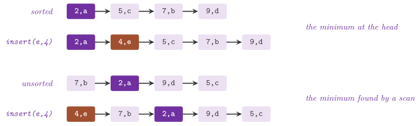
§10.1.1. On the sorted list the
least item is the head, and min() and deleteMin() cost \(O( 1 )\).
Instead, insert() scans from the head for the first cell of larger priority
and inserts before it, which keeps the items of equal priority in the
order of their insertions; decrease() takes the cell out and inserts it
again, both in \(O( n )\) time, and since the item then lies in a new cell it
writes the new position into the handle, which it takes by reference. On the unsorted list insert() puts the new
cell at the head and decrease() changes the priority in place, in
\(O( 1 )\), while min() and deleteMin() scan the whole list for the
first cell of least priority (Figure 9.1). In
both, the handle is the position of the cell, which the list keeps valid
while the cell is in it (on the sorted list, until a decrease() moves the
item and updates the handle).
The public members of ListPriorityQueue are the following:
// declarations of <ADS/priority/ListPriorityQueue.h>
template< class T , std::totally_ordered P = int , bool Sorted = true >
class ListPriorityQueue
{
 public:
 using Handle = typename List< Pair >::Pos;
 bool empty( void ) const;
 int size( void ) const;
 const T & min( void ) const;
 T deleteMin( void );
 Handle insert( const T & x , const P & p );
 void decrease( Handle & y , const P & p );
 };
Algorithm 9.1. The operations of
ListPriorityQueue (Montresor 2025,
§10.1.1); \(L\) is the list.
TreePriorityQueue keeps the items in a Red-Black tree (cf.
chapter 8) under the keys \(( p , i )\), where \(i\) is the
number of the insertion of the item (Montresor 2025,
§10.1.2). Indeed, the number makes the keys
distinct, since a search tree is a dictionary and two items of the same
priority would otherwise collide, and it orders the items of equal priority
by their insertions. Its handle is \(i\), and a vector \(\mathit{pr}\)
of the priorities by number gives the key under which decrease() finds
the node, removes it and inserts it again with the new priority. Since the least
item is the leftmost node and the height of the tree is
\(O( \log n )\), each operation takes \(O( \log n )\) time (min() included,
since the tree does not cache its leftmost node).
The public members of TreePriorityQueue are the following:
// declarations of <ADS/priority/TreePriorityQueue.h>
template< class T , std::totally_ordered P = int >
class TreePriorityQueue
{
 public:
 using Handle = long;
 bool empty( void ) const;
 int size( void ) const;
 const T & min( void ) const;
 T deleteMin( void );
 Handle insert( const T & x , const P & p );
 void decrease( Handle y , const P & p );
 };
Of the realizations of the chapter, only the tree and the sorted list
have a view (i.e., the range begin(), end() of the standard interface)
that gives the items in increasing order of priority. The views of the
heaps give the items "in no useful order" but for the first.
9.3 The binary heap¶
A complete binary tree is one whose levels are full but for the last, whose nodes are as far to the left as possible. Such a tree needs no pointer: its nodes can be laid out in a vector by levels, from the root and from left to right within a level (the breadth-first order), and the place of a node then determines the places of its parent and of its children. We name the layout after Eytzinger, who used it in 1590 for the family trees of the princes of Europe (Eytzinger 1590; Morin 2013, §10.1), and it is shown in Figure 9.2.
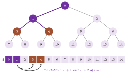
Lemma 9.1. In the layout of Eytzinger of a complete \(d\)-ary tree, the children of the place \(i\) are the places \(d i + 1 , \ldots , d i + d\), and the parent of the place \(i > 0\) is \(\lfloor ( i - 1 ) / d \rfloor\); for \(d = 2\), the left child is \(2 i + 1\), the right one \(2 i + 2\) and the parent \(\lfloor ( i - 1 ) / 2 \rfloor\).
Proof. In the breadth-first order the children of a node come after those of the nodes before it. Hence the places before the first child of \(i\) hold the root and the children of the places \(0 , \ldots , i - 1\), i.e., \(1 + d i\) places, and the first child of \(i\) is the place \(d i + 1\), followed by the others. Conversely, the place \(c = d i + j\) with \(1 \le j \le d\) gives \(\lfloor ( c - 1 ) / d \rfloor = i\), since \(0 \le j - 1 < d\). \(\square\)
A heap is a tree whose nodes are heap-ordered: no node has a priority smaller than that of its parent, and hence the root holds a minimum. In the binary heap of Williams 1964, a complete binary tree in the layout of Eytzinger is heap-ordered. It is thus a vector \(A[ 0 .. n - 1 ]\) with
Note that (9.2) is much weaker than the order of a sorted vector: it puts no constraint on two items neither of which is an ancestor of the other. It can therefore be restored, after a change, along a single path from the root, which is short since the tree is complete.
Lemma 9.2. A heap of \(n \ge 1\) items with \(d\) children per node has height
i.e., \(h = \lfloor \log_2 n \rfloor\) for \(d = 2\) and \(h = \Theta( \log_d n )\) in general.
Proof. The levels \(0 , \ldots , h - 1\) are full and hold \(1 + d + \cdots + d^{h - 1} = ( d^h - 1 ) / ( d - 1 )\) items, fewer than \(n\), while the levels \(0 , \ldots , h\), if full, would hold \(( d^{h + 1} - 1 ) / ( d - 1 ) \ge n\) items. Hence \(d^h < ( d - 1 ) n + 1 \le d^{h + 1}\), and taking the logarithms gives (9.3). For \(d = 2\) this reads \(2^h \le n < 2^{h + 1}\). \(\square\)
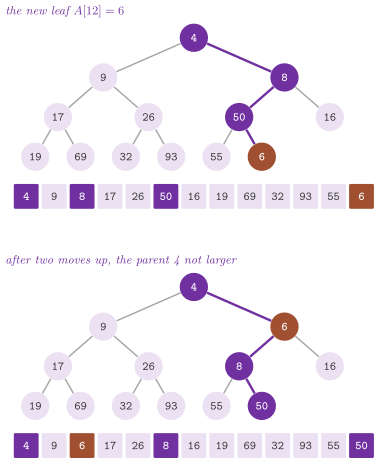
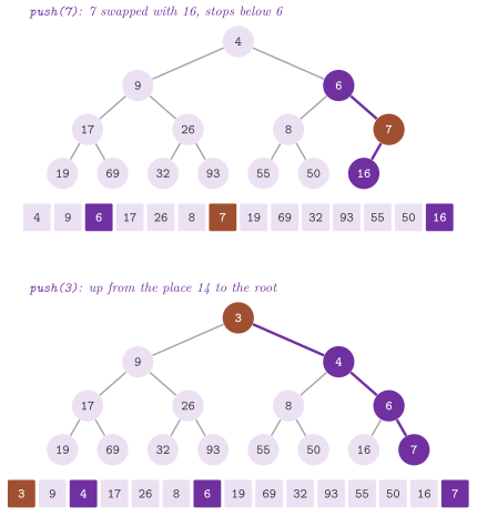
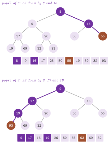
We can now describe the operations. An item pushed goes to the first free
place, \(A[ n ]\), which is a leaf and keeps the tree complete; (9.2) can then fail only between the new item
and its parent, and the item is moved up, swapping it with its parent
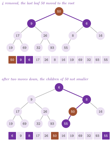
while it is smaller (Figure 9.3). To remove the
minimum, the last item \(A[ n - 1 ]\) is moved to the root, which keeps the
tree complete, and is then moved down, swapping it with the smaller of its
children while that child is smaller than it
(Figure 9.4). Algorithm 9.2
gives both for \(d\) children per node as HeapPriorityQueue makes them,
the walk down being the minHeapRestore() of Montresor 2025,
§10.1.3.
Algorithm 9.2. The operations of
HeapPriorityQueue (Montresor 2025,
§10.1.3): \(H[ 0 .. n - 1 ]\) is the
vector of the items, each of which records its place \(\mathit{pos}\).
Lemma 9.3. If (9.2) holds before them,
insert(), decrease() and deleteMin() leave a heap, the first two
after at most \(h\) swaps of one comparison each and the third after at most
\(h\) swaps of \(d\) comparisons each; hence they cost \(O( \log_d n )\),
\(O( \log_d n )\) and \(O( d \log_d n )\) time.
Proof. During the walk up from the place \(i\), (9.2) holds everywhere but possibly between \(A[ i ]\) and its parent; moreover, the parent of \(i\) is not larger than the children of \(i\), since the item at \(i\) is the only one that changed and it only decreased. A swap of \(A[ i ]\) with its larger parent moves the only violation one level up, and the walk stops at the root or where the parent is not larger. In the walk down, (9.2) holds everywhere but possibly between \(A[ i ]\) and its children; the smaller child, moved up, is not larger than its sibling and not smaller than the old parent of \(i\), and the violation moves one level down. A level costs one comparison up and \(d\) down (\(d - 1\) among the children, one with the item), and there are at most \(h\) levels (Lemma 9.2). \(\square\)
The handle that insert() returns is the item itself, allocated once,
which records its place in the vector; each swap updates the places of
the two items it moves, and thus decrease() finds its item in \(O( 1 )\)
and moves it up as insert() does (Montresor 2025, exercise
10.6 for \(d > 2\)). Beyond the book,
the items come from an ObjectPool of the queue (cf.
chapter 5), which takes back the item of
deleteMin() for the next insert(), so that an item costs no call to
the allocator and the items in use stay close in memory. As in the book,
the capacity \(c\) is fixed when the queue is built, and an insert() into
a full queue violates its precondition. Its template takes the item, the priority and \(d\), 2 by default; priorities() gives the
priorities in the order of the vector, against which the tests compare the
figures of the book.
We can now summarize the binary heap in the form of Morin 2013, Theorem 10.1.
Theorem 9.1. A binary heap realizes the
priority queue with push() and pop() in \(O( \log n )\) time and top()
in \(O( 1 )\); on a vector that doubles when full, any sequence of \(m\)
pushes and pops from the empty heap spends \(O( m )\) time in all the
enlargements.
Proof. The first part is Lemma 9.3 with \(d = 2\). The second is the argument of Lemma 3.3, since a push adds one place and an enlargement moves the items of a full vector. \(\square\)
Since a heap holds its items in a vector, it can be built from \(n\) given
items faster than by \(n\) pushes: the construction of Floyd
1964, the heapBuild() of Montresor
2025, §10.1.4, takes the items in
any order and moves each internal node down, from the last one to the
root, since the leaves are heaps of one item already. This is the
assign() of DaryHeap (§9.4), whose
pseudocode follows, and the first phase of heapsort (cf.
chapter 12).
Lemma 9.4. The construction of Floyd makes a heap of \(n\) items with \(d\) children per node in \(O( n )\) time, with at most \(d^2 n / ( d - 1 )\) comparisons, i.e., \(4 n\) for \(d = 2\).
Proof. When the node \(i\) is moved down, its subtrees are heaps, since their roots have larger places and were moved down before it; the walk down of Lemma 9.3 then makes the subtree of \(i\) a heap. A node of height \(j\) (the length of the longest path from it to a leaf) costs at most \(d j\) comparisons. Its subtree is full down to the depth \(j - 1\) below it and has a node at the depth \(j\), i.e., it holds at least \(( d^j - 1 ) / ( d - 1 ) + 1 \ge d^j / ( d - 1 )\) nodes, and the subtrees of the nodes of height \(j\) are disjoint; hence at most \(( d - 1 ) n / d^j\) nodes have height \(j\), and the comparisons are at most \(\sum_{j \ge 1} d j ( d - 1 ) n / d^{j} = d ( d - 1 ) n \cdot ( 1 / d ) / ( 1 - 1 / d )^2 = d^2 n / ( d - 1 )\). \(\square\)
A heap of \(n\) items is thus built in linear time, whereas reading the items of a heap in order costs \(\Omega( n \log n )\) comparisons (cf. chapter 12): the order of a heap holds much less information than that of a sorted vector, which is also why a heap can be kept up to date with a logarithmic number of comparisons per operation.
Two exercises of Morin 2013, §10.3 illustrate a binary heap. We solve them in Figure 9.5 and Figure 9.6, on the heaps that end Figure 9.3 and Figure 9.4.
9.4 Heaps with d children and plain items¶
DaryHeap< T , Better , D , BottomUp > is the heap of
§9.3 with \(D\) children per node, \(D = 4\) by default,
whose items are plain values ordered by better(), with no handle and no
decrease(). Its items are meant to be "small" and to carry their keys (e.g.,
the two costs of a node of a search and a pointer to it), and a comparison
then never follows a pointer. Also, the vector of a large heap is on huge
pages (cf. chapter 5), and a walk from the root to a leaf
does not miss the translation buffer at each level. With \(D = 2\) it is the
BinaryHeap of Morin 2013, §10.1, with any
\(D\) it is the DaryHeap of Morin 2013, exercise
10.5, and its static functions parent( i )
and child( i , j ) are the formulae of Lemma 9.1,
which solve Morin 2013, exercise 10.4.
Our code differs from that of Morin 2013,
§10.1 in three points, each of which
saves work on a real machine. First, the walks move a hole instead of
swapping the item at each level: the item is kept aside, each step copies
one item into the hole and moves the hole, and the item is written once
where the walk stops, one write per level instead of the three of a swap.
Second, the item travels as a value, never stored in the vector and read
back, which would stall the forwarding of the store to the load at each
level. Third, the vector is not shrunk when it is a third full, as in the
book, so that a heap keeps the memory of its largest size and never copies
its items to shrink. The walk down (the core of pop() and of the
construction) compares the children with each other and the best of them
with the item, \(D\) comparisons per level (lines 4 to 7 of the pseudocode
of pop() above).
The choice of \(D\) trades the comparisons of pop() against the levels
that both operations walk, which is the analysis that Morin 2013,
exercise 10.5 is about.
Lemma 9.5. A push() into a \(D\)-ary heap of
\(n\) items makes at most \(\log_D( ( D - 1 ) n + 1 )\) comparisons, and a
pop() at most \(D\) times as many; hence a pop() makes about
\(D \log_D n = ( D / \log_2 D ) \log_2 n\) comparisons, which is least for
\(D = 3\) among the integers, and is the same for \(D = 4\) as for \(D = 2\).
Proof. The bounds are those of Lemma 9.3 with the height of Lemma 9.2. The function \(D / \log_2 D\) takes the values 2, \(3 / \log_2 3 \approx 1.89\), 2 and \(5 / \log_2 5 \approx 2.15\) for \(D = 2 , 3 , 4 , 5\), and it increases for \(D \ge 3\), since its derivative has the sign of \(\ln D - 1\). \(\square\)
This is why \(D = 4\) is the default. A heap of four children per node is
half as deep as a binary one: a push walks half as many levels, and a pop
makes no more comparisons than in the binary heap. Furthermore, the four
children of a node are consecutive, 64 bytes for items of 16 bytes, and
they span at most two lines of the cache. Note that the code does not
align them: the children of \(i\) start at the place \(4 i + 1\), i.e., at 16
bytes past a multiple of 64 when the vector starts on a line, so that with
items of 16 bytes they always straddle two lines; the analyses of the
caches that count one miss per level shift the array by three places to
align them (LaMarca
and Ladner 1996; Larkin, Sen and
Tarjan 2014). When the decreases
dominate, as in the algorithm of Dijkstra with a heap that has
decrease(), the best \(D\) is larger.
Lemma 9.6. With \(m\) decreases and \(n\) extractions, a \(d\)-ary heap costs
which for \(m \ge n\) and \(d = \max\{ 2 , \lceil m / n \rceil \}\) is \(O( m \log_{2 + m / n} n )\), i.e., \(O( m )\) on the graphs with \(m = \Omega( n^{1 + \varepsilon} )\) for a constant \(\varepsilon > 0\) (Johnson 1975).
Proof. (9.4) is Lemma 9.3 summed over the operations. With \(d\) as stated, \(n d \le m + 2 n\), and both terms are \(O( ( m + n ) \log_d n ) = O( m \log_d n )\), while \(\log_d n \le 2 \log_{2 + m / n} n\) since \(2 + m / n \le 2 d \le d^2\); if \(m = \Omega( n^{1 + \varepsilon} )\), then \(\log_d n = O( 1 / \varepsilon )\). \(\square\)
With BottomUp, pop() takes the walk from the bottom up of Floyd
1964 and Wegener
1993. The hole of the root moves down
to a leaf along the best children, with \(D - 1\) comparisons per level and
none with the item that will fill it; the last item then moves up from
that leaf as in push(). Since it was a leaf, the last item usually
belongs near the bottom, the climb is short, and the walk saves about one
comparison per level. It may lose when the item would have stopped halfway
down, as in the hold model of the simulations, where the item removed is
followed by a push of a similar key. Both walks are checked by the test
heaps.dary-heap-bottom-up, against
std::priority_queue.
Beyond the book, DaryHeap solves three exercises of Morin 2013,
§10.3, which we take in his order. We begin
with the removal of the item in a given place, erase( i ) (exercise 10.3).
Lemma 9.7. Let the item at the place \(i\) of a
heap be removed and the last item \(x\) be put in its place. If \(x\) is smaller
than the parent of \(i\), the walk up from \(i\) restores the heap, and otherwise
the walk down does; only one walk is needed, and erase( i ) costs
\(O( D \log_D n )\) time.
Proof. The items below \(i\) are not smaller than the item removed, which
is not smaller than the parent of \(i\). If \(x\) is smaller than that parent,
it is smaller than all the items below \(i\), and (9.2) fails only between
\(x\) and its ancestors, which the walk up mends as in push(). Otherwise
\(x\) is not smaller than its parent, and (9.2) fails only between \(x\) and
its children: \(x\) may come from another subtree, where it was larger than
the items below \(i\), and the walk down mends it as in pop(). \(\square\)
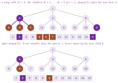
Figure 9.7 shows a heap with \(D = 3\) and the case of
the walk down. As for why erase( i ) is of little use, the places of the
items change at each operation and the heap gives no handle to follow them. A
caller must thus first search for the place of an item, in \(O( n )\) time, more
than any operation of the heap costs. In IndexedDaryHeap
(§9.5) the items know their places, and the same
removal costs \(O( D \log_D n )\) in all.
Exercise 10.9 is about the second least item, which secondTop() gives as the
best of the children of the root in \(O( D )\) time (a null pointer if the heap
has fewer than two items): any other item has one of the children of the root
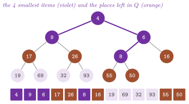
as an ancestor, and is not smaller than it. Exercise 10.10 is about the \(k\)
least items in order, which smallest( k ) gives without changing the heap,
by a second heap \(Q\) of places that starts with the root and receives the
children of each place it gives.
Lemma 9.8. smallest( k ) gives the \(k\) least
items of a \(D\)-ary heap in order, in \(O( k D \log ( k D ) )\) time, i.e.,
\(O( k \log k )\) for a constant \(D\); its heap \(Q\) never holds more than
\(k ( D - 1 ) + 1\) places.
Proof. By induction on the items given: \(Q\) always holds the places whose parent has been given but which have not been given themselves (the root at the start). Any item not yet given has an ancestor in \(Q\), which is not larger than it, and therefore the least item of \(Q\) is the least item not yet given. A step removes one place from \(Q\) and puts in at most \(D\); hence \(|Q| \le 1 + k ( D - 1 )\), and an operation of \(Q\) costs \(O( \log ( k D ) )\). \(\square\)
Figure 9.8 shows the answer for \(k = 4\) on the
binary heap of Figure 9.3, and the five places left
in \(Q\), which are exactly \(k ( D - 1 ) + 1\). Of course, the \(k\)-th least item
of the exercise is the last item that smallest( k ) gives.
The merge of \(k\) sorted lists of Morin 2013, exercise
10.11 is another use of the heap of plain
items. A heap of the pairs (first item, list) gives the next item of the merge
at each pop(), which is followed by a push() of the next item of the same
list. Since the heap holds at most \(k\) pairs, the merge of \(n\) items costs
\(O( n \log k )\). In the test ods_ints.ods.ex10.11.k-way-merge we make it
with a DaryHeap and compare the result with that of multiwayMerge(), which
does it with fewer comparisons per item (§9.11).
Finally, assign( first , last ) replaces the items of the heap by those of a
range, arranged by the construction of Floyd (Lemma
9.4), and leaves the heap unchanged if a copy throws.
reserve( n ) and clear() are those of the vector, and the view gives the
items in the order of the vector, the root first.
9.5 Heaps of indices and heaps with pointers¶
The algorithms on graphs know their items by number: the nodes
\(0 , \ldots , n - 1\). IndexedDaryHeap< K , D > is a \(D\)-ary heap of such
ids, \(D = 4\) by default, whose items are the pairs Entry of a key and an id.
With the key inline, a comparison never leaves the vector of the heap. A
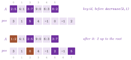
second vector \(\mathit{pos}\) holds the places of the ids (\(-1\) for an id that
is not in the heap), and takes the place of the handles of
HeapPriorityQueue: each move of an item updates the place of its id, and the
operations on an id start from its place, read in \(O( 1 )\). With \(s\) items in
the heap, push( id , k ) and decrease( id , k ) move the item up in
\(O( \log_D s )\) time, while pop() and top() work as in DaryHeap.
increase( id , k ) moves the item down as pop() moves the last item, in
\(O( D \log_D s )\), and update( id , k ) takes either way as the new key
requires. Finally, erase( id ) puts the last item in the place of the id and
moves it up or down by Lemma 9.7 (Figure
9.9).
The public members of IndexedDaryHeap are the following:
// declarations of <ADS/priority/IndexedDaryHeap.h>
template< class K , unsigned D = 4 , class Policy = NoObservers ,
          class A = std::allocator< K > >
class IndexedDaryHeap
{
 public:
 struct Entry
 {
  K key;
  int id;
  };
 using Handle = int;
 template< class... O >
 explicit IndexedDaryHeap( int n = 0 , O &... o );
 void reset( int n );
 void grow( int n );
 int ids( void ) const;
 bool empty( void ) const;
 std::size_t size( void ) const;
 bool contains( int id ) const;
 const K & key( int id ) const;
 void push( int id , const K & k );
 void decrease( int id , const K & k );
 void increase( int id , const K & k );
 void update( int id , const K & k );
 void erase( int id );
 bool pushOrDecrease( int id , const K & k );
 const Entry & top( void ) const;
 Entry pop( void );
 void clear( void );
 Handle insert( int id , const K & k );
 int min( void ) const;
 int deleteMin( void );
 Subject & subject( void );
 template< class O >
 int attach( O & o )
  requires( Subject::dynamic );
 void detach( int id )
  requires( Subject::dynamic );
 };
Its space is that of the \(s\) entries and of the \(n\) places, i.e., \(e s + 4 n\)
bytes for entries of \(e\) bytes and ids of 4 bytes: \(e = 8\) for keys of 4 bytes
and \(e = 16\) for keys of 8, the entry being padded to the alignment of its
key. With 32-bit keys and \(D = 4\), the four children of a node take half a
line of the cache. pushOrDecrease( id , k ) pushes an id that is not in the
heap and lowers the key of one that is (the relaxation of an edge in the
algorithm of Dijkstra), and returns whether the key changed. contains(),
key(), ids(), reset( n ) (the heap of \(n\) ids emptied, its memory kept),
grow( n ) and clear() complete the interface. grow( n ) raises the range
of the ids to \([ 0 , n )\) keeping the items, the new ids absent; the vector
\(\mathit{pos}\) at least doubles when it is full, so that a search that numbers
its nodes as it generates them grows the heap with them in \(O( 1 )\) amortized
time per node (test engineered_search.indexed-heap-grow). Also, the heap
models the concept PriorityQueue, the ids being their own handles:
insert() is push(), min() the id of top() and deleteMin() that of
pop(). Hence the algorithms of chapter 14 run on it
unchanged (test engineered_graph.indexed-dary-heap). A search may also need
to take a node out of its frontier, or to make it worse when a bound prunes
it, which erase() and increase() do (test
engineered_search.indexed-heap-erase). The last parameter, Policy, is the
subject policy of §1.13, by which the heap
tells its insertions, erasures and changes of key, and on demand the moves of
its items (§1.15.1); with NoObservers, the
default, its code is that of the plain heap.
Some searches choose a node by one key and must know at each moment the least
of a second key over the whole frontier. A bounded suboptimal search expands
by an inflated cost or by the estimated distance to the goal, and needs the
least lower bound \(f_{\min}\) of the open nodes to stop or to certify its
factor of suboptimality (Pearl and Kim
1982; Thayer and Ruml
2011). Similarly, a branch and bound by
best estimate selects by an estimate and prunes by the least bound.
IndexedHeapPair< K , Bd , D > keeps the same ids in two IndexedDaryHeap,
\(H_K\) by the keys and \(H_B\) by the bounds. top() and topKey() read the
root of \(H_K\), minBound() and minBoundId() that of \(H_B\), and bound()
the bound of an id. Also, push( id , k , b ) pushes into both heaps,
update( id , k , b ) and erase( id ) change both, and pop() (resp.
popMinBound()) pops from one heap and erases the same id from the other by
Lemma 9.7. The other members, contains(), key(),
size(), ids(), reset( n ) and clear(), are those of IndexedDaryHeap,
read or applied to both heaps.
The public members of IndexedHeapPair are the following:
// declarations of <ADS/priority/IndexedHeapPair.h>
template< class K , class Bd = K , unsigned D = 4 >
class IndexedHeapPair
{
 public:
 explicit IndexedHeapPair( int n = 0 );
 void reset( int n );
 int ids( void ) const;
 bool empty( void ) const;
 std::size_t size( void ) const;
 bool contains( int id ) const;
 const K & key( int id ) const;
 const Bd & bound( int id ) const;
 void push( int id , const K & k , const Bd & b );
 void update( int id , const K & k , const Bd & b );
 void erase( int id );
 int top( void ) const;
 const K & topKey( void ) const;
 const Bd & minBound( void ) const;
 int minBoundId( void ) const;
 int pop( void );
 int popMinBound( void );
 void clear( void );
 };
Thus an operation costs two walks, \(O( D \log_D s )\), but for push(),
which costs two walks up. The alternative is a heap of the bounds with lazy
deletion, in which the ids popped by the key stay until they reach its
top. It saves the second walk of pop(); however, it may keep \(O( m )\)
stale entries for \(m\) operations, which minBound() must skip, and an id
pushed again needs a stamp to tell its copies apart. Instead, the pair keeps \(s\)
entries in each heap, and the bound of an id is always the one it has (test
engineered_search.indexed-heap-pair). We remark that a frontier read in
order from its least item and changed anywhere is better kept in an
ordered dictionary with iterators, such as the B-tree of
chapter 8. A frontier that is only popped is better
kept in a heap, whose items need no order beyond the least one.
LinkedHeapPriorityQueue< T , P , L > keeps the shape of the binary heap on
nodes linked to their parent and to their two children, instead of on a
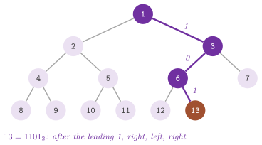
vector. In the numbering by levels from 1 (that of Eytzinger shifted by one),
the node \(k\) has the children \(2 k\) and \(2 k + 1\). Hence the path from the
root to the node \(k\) is spelled by the bits of \(k\) after the leading one, 0
for the left child and 1 for the right one (Figure
9.10). In \(O( \log n )\) steps, insert() finds the
parent of the new leaf \(n + 1\) and deleteMin() the last leaf \(n\). Items move
up and down by swapping the contents of the nodes, as in the vector, and each
operation takes \(O( \log n )\) time; there is no decrease(), which would need
a handle that follows the contents.
The public members of LinkedHeapPriorityQueue are the following:
// declarations of <ADS/priority/LinkedHeapPriorityQueue.h>
template< class T , std::totally_ordered P = int , bool L = false >
class LinkedHeapPriorityQueue
{
 public:
 LinkedHeapPriorityQueue( void );
 bool empty( void ) const;
 int size( void ) const;
 const T & min( void ) const;
 const P & minPriority( void ) const;
 void insert( const T & x , const P & p );
 T deleteMin( void );
 };
With L true the heap keeps instead a pointer to the last leaf and finds
the place of the next one by walking the tree (nextParent() above). The
new leaf is the right sibling of the last one if this is a left child.
Otherwise one goes up while on a right child, then, unless at the root, to
the right sibling, and down along the left children. After deleteMin()
the new last leaf is found symmetrically. Both walks take \(O( \log n )\)
steps and need no count of the nodes, which is the form of the exercise of
the linked heap (test beyond.linked-heap). The nodes come from an
ObjectPool of the queue, as in HeapPriorityQueue (test
heaps.linked-heap-pool). Its view walks the tree in symmetric order by a
PathIterator, to which the class Shape gives the root, the children
(left() and right()) and the contents of a node (read()); this order is of no use but for visiting all
the items.
9.6 The randomized meldable heap¶
A heap in a vector cannot merge with another heap faster than by rebuilding
it, in linear time, and one may well need such merges (e.g., in the algorithms
that join the queues of two components). MeldableHeap< T , Less , A > is the
randomized meldable heap of Gambin and Malinowski
1998, as Morin 2013,
§10.2 presents it: a heap-ordered binary
tree of nodes with pointers, of any shape, whose only structural operation is
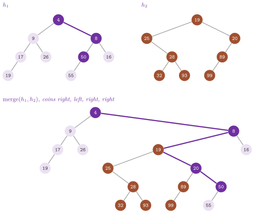
the merge of two such trees. Given the roots \(h_1\) and \(h_2\), the merge keeps
the smaller root on top (say \(h_1\), after exchanging the two if needed) and
merges \(h_2\), recursively, with one of the two subtrees of \(h_1\), chosen by a
fair coin (Figure 9.11). Then push( x ) merges
the heap with a tree of one node, pop() merges the two subtrees of the root,
meld( o ) merges a whole heap o into this one, leaving o empty. Finally,
erase( h ) removes the node of the handle \(h\) that push() returned. Each
of these operations makes a constant number of merges.
The public members of MeldableHeap are the following:
// declarations of <ADS/priority/MeldableHeap.h>
template< class T , class Less = std::less< T > ,
          class A = std::allocator< T > >
class MeldableHeap
{
 public:
 using Handle = Node *;
 explicit MeldableHeap( Less less = Less() , std::uint64_t seed = 1 ,
                        const A & alloc = A() );
 Handle push( T x );
 const T & top( void ) const;
 const T * secondTop( void ) const;
 T pop( void );
 T erase( Handle h );
 void meld( MeldableHeap & o );
 std::vector< T > smallest( std::size_t k ) const;
 std::size_t size( void ) const;
 bool empty( void ) const;
 void clear( void );
 static const T & get( Handle h );
 };
Algorithm 9.3. The merge of MeldableHeap
(Morin 2013, §10.2), its recursion
made a loop that hangs each node by the link that will hold it.
Our analysis rests on the length of a random walk in a binary tree: a walk that starts at the root, goes at each step to the left or to the right child by a fair coin, and ends when it leaves the tree. Rather surprisingly, one can bound its length independently of the shape of the tree.
Lemma 9.9. In a binary tree of \(n\) nodes, the expected length of a random walk from the root is at most \(\log_2( n + 1 )\) (Morin 2013, Lemma 10.1).
Proof. By induction on \(n\); for \(n = 0\) the walk has length \(0 = \log_2 1\). With \(n_1\) and \(n_2 = n - 1 - n_1\) nodes in the two subtrees of the root, the walk takes one step and continues in one of them with probability \(1 / 2\) each, so that its expected length \(E\) is
by the concavity of the logarithm, \(( \log a + \log b ) / 2 \le \log ( ( a + b ) / 2 )\). \(\square\)
A second proof, also in Morin 2013, §10.2, goes through the entropy. A binary tree of \(n\) nodes has \(n + 1\) external nodes (the empty subtrees), and the walk ends at the external node \(i\), of depth \(d_i\), with probability \(p_i = 2^{-d_i}\); hence its expected length is \(\sum_i p_i d_i = \sum_i p_i \log_2( 1 / p_i )\), the entropy of a distribution over \(n + 1\) outcomes, which is at most \(\log_2( n + 1 )\).
Lemma 9.10. The merge of two heaps of \(n_1\) and \(n_2\) nodes takes \(O( \log n_1 + \log n_2 )\) expected time, whatever their shapes (Morin 2013, Lemma 10.2).
Proof. Each step of the merge takes one step of a random walk in one of the two heaps, the one whose root is on top, from that root to one of its children, and the merge ends as soon as one of the two walks leaves its tree. Since the coins of the two walks are independent of the shapes, the expected number of steps is at most \(\log_2( n_1 + 1 ) + \log_2( n_2 + 1 )\) by Lemma 9.9. \(\square\)
Theorem 9.2. MeldableHeap realizes the
priority queue with push(), pop(), meld() and erase() in
\(O( \log n )\) expected time and top() in \(O( 1 )\) (Morin 2013, Theorem
10.2).
Proof. Each of the four operations makes one merge of two trees of at most \(n\) nodes (Lemma 9.10). \(\square\)
The removal of the node \(u\) of a handle (Morin 2013, exercise 10.8) merges the two subtrees of \(u\) and hangs the result where \(u\) was, since the order holds between the parent of \(u\) and each node below \(u\); the walk of the merge starts at the subtrees of \(u\), with fewer than \(n\) nodes.
The second least item (Morin 2013, exercise
10.9) is the smaller of the two children of
the root, which secondTop() gives in \(O( 1 )\). The \(k\) least items in order
(Morin 2013, exercise 10.10) come from
smallest( k ), the algorithm of Lemma 9.8 on the
nodes instead of the places. Its heap of nodes holds at most \(k + 1\) of them,
since each step takes one and puts two, and it costs \(O( k \log k )\) time
without changing the heap. get( h ) reads the item of a handle.
This code differs from that of Morin 2013,
§10.2 in four points. First, the merge
is a loop, with no recursion, which hangs each node by a pointer to the
link that will hold it. A heap of \(10^6\) items pushed in increasing order
(whose expected depth is logarithmic, but whose worst depth is not) thus
never overflows the stack of the calls; the destructor and clear() are
iterative as well. Second, the coins are the bits of one word of SplitMix64 (cf.
chapter 7), used one at a time, 64 coins per word,
where the book calls rand() for each; the seed of the generator is an
argument of the constructor (1 by default), so that a heap is reproducible. Third, the nodes come from the
allocator A (e.g., a PoolAllocator, cf. chapter 5),
and two heaps meld only if their allocators are equal: each node must go
back to the allocator that gave it. Fourth, the items are moved, not
copied, into the nodes and out of them.
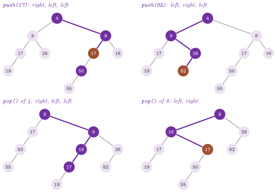
Two exercises of Morin 2013, §10.3
illustrate the meldable heap with a coin; we solve them in
Figure 9.12, with the coins written in its
caption. Since the shape of the heap depends on the coins, the
test ods_ints.ods10.2.meldable-heap, whose coins are those of a seeded
generator, checks instead the items that come out and the second least
item, which do not depend on them.
9.7 Fibonacci heaps¶
On a graph of \(n\) nodes and \(m\) edges, the algorithms of Dijkstra and Prim
make up to \(m\) decreases and \(n\) extractions, and on a dense graph the
decreases dominate. The Fibonacci heap of Fredman and Tarjan
1987, which Montresor 2025,
§11.5 names for the shortest paths
without describing it, lowers the cost of decrease() to \(O( 1 )\) amortized
by doing almost nothing at each operation and tidying the heap only in
deleteMin(). FibonacciHeapPriorityQueue< T , P > is a collection of
heap-ordered trees whose roots lie in a circular doubly linked list, with a
pointer \(\mathit{min}\) to the least root; the children of each node lie in a
circular list as well, and each node records its parent, its degree (the
number of its children) and a mark, set when the node, not a root, loses a
child.
insert() adds a tree of one node to the list of the roots. decrease()
lowers the priority of a node and, if the node became smaller than its
parent, cuts it, making it a root with its subtree; a parent that loses
a second child since it became a child is cut in turn, and so on upwards
(the cascading cut), the mark recording the first loss. deleteMin()
removes the least root, moves its children among the roots, and then
consolidates the roots, linking two roots of equal degree, the larger
under the smaller, until all the degrees differ
(Figure 9.13).
The public members of FibonacciHeapPriorityQueue are the following:
// declarations of <ADS/priority/FibonacciHeapPriorityQueue.h>
template< class T , std::totally_ordered P = int ,
          class A = HugePageAllocator< T > >
class FibonacciHeapPriorityQueue
{
 public:
 using Handle = Node *;
 FibonacciHeapPriorityQueue( void );
 explicit FibonacciHeapPriorityQueue( const A & alloc );
 bool empty( void ) const;
 int size( void ) const;
 const T & min( void ) const;
 const P & minPriority( void ) const;
 Handle insert( const T & x , const P & p );
 T deleteMin( void );
 void decrease( Handle x , const P & p );
 };
Algorithm 9.4. The operations of
FibonacciHeapPriorityQueue (Fredman and Tarjan
1987).
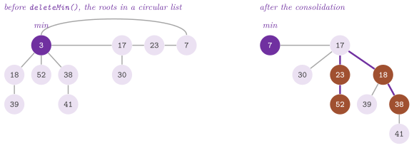
We first bound the degrees of the trees, which keep the consolidation short; in fact, it is the cascading cut that keeps them logarithmic. Let \(F_k\) be the \(k\)-th number of Fibonacci, \(F_0 = 0\), \(F_1 = 1\), \(F_{k + 2} = F_{k + 1} + F_k\), and \(\phi = ( 1 + \sqrt{5} ) / 2\) the golden ratio.
Lemma 9.11. A node of degree \(k\) in a Fibonacci heap has at least \(F_{k + 2} \ge \phi^k\) nodes in its subtree, itself included; hence the largest degree \(D( n )\) of a heap of \(n\) nodes is at most \(\log_\phi n\).
Proof. Take the children of a node \(x\) in the order in which they were linked to it. When the \(i\)-th child \(y_i\) was linked, \(x\) had at least \(i - 1\) children, and \(y_i\) had the same degree as \(x\), since only roots of equal degree are linked. Since then \(y_i\) has lost at most one child, or it would have been cut, and hence its degree is at least \(i - 2\). Let \(s_k\) be the least size of a subtree whose root has degree \(k\); then \(s_0 = 1\), \(s_1 = 2\) and \(s_k \ge 2 + \sum_{i = 2}^{k} s_{i - 2}\), counting \(x\) and its first child. Since \(F_{k + 2} = 1 + \sum_{i = 0}^{k} F_i\), induction gives \(s_k \ge F_{k + 2}\), and \(F_{k + 2} \ge \phi^k\) by induction from \(\phi^2 = \phi + 1\). \(\square\)
Theorem 9.3. Starting from an empty
Fibonacci heap, insert() and min() cost \(O( 1 )\), decrease() costs
\(O( 1 )\) amortized and deleteMin() \(O( \log n )\) amortized; the
algorithm of Dijkstra thus runs in \(O( m + n \log n )\) time (Fredman and
Tarjan 1987).
Proof. Let \(t\) be the number of trees and \(\mu\) that of the marked nodes, and take the potential
insert() raises \(\Phi\) by 1 and costs \(O( 1 )\). A decrease() that makes
\(c\) cuts costs \(O( c )\). It adds \(c\) trees, clears the marks of at least
\(c - 1\) nodes (each cut of the cascade but the first is of a marked node)
and sets at most one; hence \(\Phi\) changes by at most
\(c + 2 ( 2 - c ) = 4 - c\), and the amortized cost is \(O( 1 )\). In
deleteMin(), the children of the minimum (at most \(D( n )\)) join the
roots, and the consolidation of \(t + D( n )\) roots costs
\(O( t + D( n ) )\), since each link removes a root. It leaves at most
\(D( n ) + 1\) trees, of distinct degrees, and \(\Phi\) decreases by at least
\(t - D( n ) - 1\), which pays for the term \(t\). Thus the amortized cost of
deleteMin() is \(O( D( n ) ) = O( \log n )\) by
Lemma 9.11. Finally, the algorithm of Dijkstra
makes \(n\) insertions and extractions and at most \(m\) decreases. \(\square\)
Beyond the book, the nodes come from an ObjectPool of the heap, which
takes back the node of deleteMin() for the next insert(). Also, the children
of the minimum join the roots in \(O( 1 )\), by splicing their circular list
into that of the roots. Also, the consolidation walks the roots where they
lie, with the trees by degree in an array of 64 entries on the stack
(a degree is at most \(\log_\phi n\), below 64 for \(n < \phi^{64} \approx 2.4 \cdot 10^{13}\) nodes, i.e., more than a memory holds at the size of a node).
Its handle is the node; min() and minPriority() read the least root,
and the view visits the nodes in preorder over the circular lists. In
practice the constants of the Fibonacci heap are larger than those of a
heap in a vector, which is usually faster but (possibly) on "large" and
dense graphs (tests ch11.sec11.5.fibonacci, ch11.sec11.5.fibonacci-pool
and, for the algorithm of Prim, ch14.ex14.4).
9.8 Pairing heaps¶
The pairing heap of Fredman, Sedgewick, Sleator and Tarjan
1986 is the simplest of the heaps with an
efficient decrease(), and in the experiments of Stasko and Vitter
1987 and of Larkin, Sen and Tarjan
2014 the fastest one with pointers in
practice. PairingHeap< T , P , Aux > is one heap-ordered tree in the form
child-sibling. Each node points to its leftmost child and to its right
sibling, and back to its left sibling (or to its parent, if it is the leftmost
child); a node is thus cut from its tree in \(O( 1 )\). Two trees are linked
by making the root of larger priority the leftmost child of the other one,
with one comparison and \(O( 1 )\) updates of the links.
insert() links a tree of one node with the root, and decrease() cuts
the node with its subtree (unless it is the leftmost child and still not
smaller than its parent) and links it with the root. deleteMin()
removes the root and joins its children by two passes. Its first pass links
them in pairs from the left, and its second links the results from the
right into one tree (Figure 9.14). No balance is kept, and hence
the analysis is that of a self-adjusting structure.
The public members of PairingHeap are the following:
// declarations of <ADS/priority/PairingHeap.h>
template< class T , std::totally_ordered P = int , bool Aux = false ,
          class A = HugePageAllocator< T > >
class PairingHeap
{
 public:
 using Handle = Node *;
 PairingHeap( void );
 explicit PairingHeap( const A & alloc );
 bool empty( void ) const;
 int size( void ) const;
 const T & min( void ) const;
 const P & minPriority( void ) const;
 Handle insert( const T & x , const P & p );
 T deleteMin( void );
 void decrease( Handle x , const P & p );
 T erase( Handle x );
 void increase( Handle x , const P & p );
 void update( Handle x , const P & p );
 };
Algorithm 9.5. The operations of
PairingHeap (Fredman et al. 1986;
Stasko and Vitter 1987 for Aux).
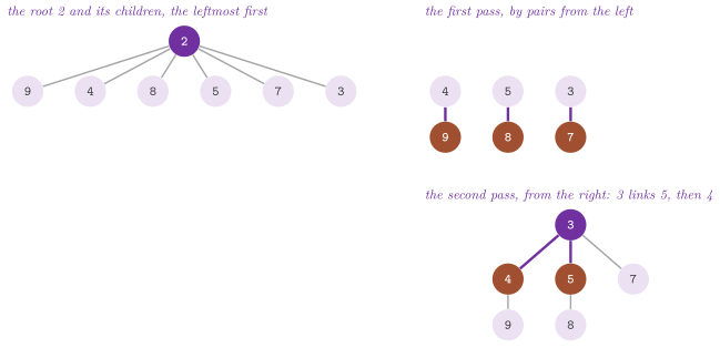
The bounds known for the two passes are \(O( \log n )\) amortized for
deleteMin() (Fredman et al. 1986),
\(O( 1 )\) amortized for insert() (Iacono
2000) and
\(O( 2^{2 \sqrt{\log \log n}} )\) amortized for decrease() (Pettie
2005). However, Fredman
1999 proved that decrease() needs
\(\Omega( \log \log n )\) amortized in this family of heaps, against the
\(O( 1 )\) of the Fibonacci heap, and a variant of Elmasry
2009 attains \(O( \log \log n )\). We do not reproduce these analyses, which take a
potential on the sizes of the subtrees (in the spirit of the splay trees of
chapter 8) and are well beyond the scope of a manual.
With Aux true the heap is the auxiliary two-pass variant of Stasko and
Vitter 1987. Here the trees of insert() and
of decrease() go to a list beside the root, with a pointer to the least
of the roots, and each costs one comparison. Then deleteMin() first
joins that list by the multipass pairing (the trees linked in pairs from
the front of a queue, each result put at its back, until one tree is
left) and links it with the root. It typically pays when the
insertions outnumber the extractions. Both passes run in place on the sibling pointers, with
no stack and no vector, and the nodes come from an ObjectPool (test
heaps.pairing-heap).
Beyond the PRIORITYQUEUE, erase() removes the node of any handle. First, the
node is cut from its siblings, its children are joined by the two passes
in its place, and the tree that results is linked with the root (or put in
the list beside it, with Aux). Hence erase() costs as a deleteMin()
on the subtree of the node, \(O( \log n )\) amortized. A raise of a priority
by increase() cannot leave the node in its place, since its children may
now be smaller than it: the node is taken out in the same way and inserted
again alone, with the same handle, at the same cost. Finally, update()
takes decrease() or increase() as the new priority requires (test
engineered_search.pairing-heap-erase).
9.9 Monotone queues of integer keys¶
On a monotone queue whose keys are "small" integers, the least key can be found by
the position of the keys in an array instead of by comparisons. The three
queues of this section have no decrease(), as in the lazy deletion of
§9.1, and a key pushed must not be smaller than
the last one extracted, \(\ell\), which is the precondition that their
contracts check.
The radix heap of Ahuja, Mehlhorn, Orlin and Tarjan
1990, RadixHeap< T , K , B >, splits a key
\(x\) of \(W\) bits into \(\lceil W / B \rceil\) digits of \(B\) bits, \(B = 4\) by
default (a signed key has its sign bit flipped, which keeps the order). It
puts the item in the bucket
where \(x_r\) is the digit \(r\) of \(x\), and \(r = 0\) if \(x = \ell\) (Figure 9.15). Its buckets are vectors used as stacks, a mask of bits marks the buckets in use, and each bucket records the least key it holds.
Lemma 9.12. Let \(x , y \ge \ell\). If the bucket of \(x\) has a smaller index than that of \(y\), then \(x < y\); and the keys of a bucket of the row \(r = 0\) are all equal.
Proof. The key \(x\) agrees with \(\ell\) above its digit \(r\), and when \(r > 0\) its digit \(r\) is larger than that of \(\ell\), since \(x > \ell\). If \(y\) lies in a higher row \(r' > r\), then \(x\) agrees with \(\ell\) on the digit \(r'\) and above, while \(y\) agrees with \(\ell\) above \(r'\) and exceeds it on the digit \(r'\); hence \(y > x\). If \(y\) lies in the same row, both agree with \(\ell\) above the digit \(r\), and their digits \(r\), i.e., the indices of the buckets, decide. In the row 0, \(x\) and \(\ell\) differ at most in the last digit, which is the index of the bucket, and two keys of one bucket are therefore equal. \(\square\)
Hence the least key is in the first bucket in use, which the mask gives by its lowest bit. If that bucket lies in the row \(r > 0\), its least key becomes the new \(\ell\), and its items move to the buckets that (9.6) gives for it, all in rows below \(r\). The other buckets, all of larger index, keep their items: a key of a row \(r' \ge r\) agrees with the new \(\ell\) on the same digits as with the old one.
The public members of RadixHeap are the following:
// declarations of <ADS/priority/RadixHeap.h>
template< class T , std::integral K = std::uint32_t , unsigned B = 4 ,
          class A = std::allocator< T > >
class RadixHeap
{
 public:
 void push( const T & x , K k );
 const T & top( void );
 K topKey( void );
 K peekKey( void ) const;
 T pop( void );
 template< class F >
 void extractBelow( K limit , F && f );
 bool empty( void ) const;
 std::size_t size( void ) const;
 void clear( void );
 };
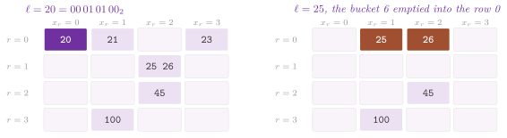
Lemma 9.13. Starting from an empty radix
heap, any sequence of \(p\) pushes and \(q\) pops costs
\(O( p \, W / B + q \, 2^B W / ( 64 B ) )\) time; hence, when every item
pushed is also popped, push() costs \(O( 1 )\) and pop()
\(O( W / B + 2^B W / ( 64 B ) )\) amortized. If every key pushed lies in
\([ \ell , \ell + C ]\) for the \(\ell\) of its push, an item moves at most
\(1 + \lceil \log_2 C \rceil / B\) times, and with \(B = 1\) a pop() costs
\(O( \log C + W / 64 )\) amortized.
Proof. An item only moves to lower rows, hence at most
\(\lceil W / B \rceil - 1\) times. With the potential
\(\Phi = \sum_x \mathrm{row}( x )\), a push raises \(\Phi\) by at most
\(\lceil W / B \rceil - 1\), each move lowers it by at least 1 and thus costs
nothing amortized, and what is left of a pop() is the scan of the mask,
\(2^B \lceil W / B \rceil\) bits in words of 64; when every item pushed is
popped, the rise of \(\Phi\) at its push can be charged to its pop instead.
In a band, a key may still lie in a high row, since a carry changes high
bits: with \(B = 1\), \(\ell = 7\) and \(x = 8\) differ in the bit 3. Let \(x\) be moved for the first time from the bucket
\(( r , x_r )\), \(r > 0\), and let \(Q\) be \(x\) with its digits below \(r\) set to
zero, a multiple of \(2^{B r}\). The old \(\ell\) has the digit \(r\) smaller than
that of \(x\) and the same digits above it, and hence \(\ell < Q\) and
\(x \le \ell + C < Q + C\). The new \(\ell\) is a key of that bucket, and so is
not smaller than \(Q\); it and every later \(\ell\) while \(x\) is in the heap lie
in \([ Q , x ]\). Let \(c = \lceil \log_2 C \rceil\). If \(C \le 2^{B r}\),
\(Q\) is also a multiple of \(2^c\), and \(x\) and every later \(\ell\) lie in one
aligned block of \(2^c\) integers. They thus differ only in their lowest \(c\)
bits, and the row of \(x\) is at most \(c / B\). If \(C > 2^{B r}\), its new
row is below \(r < c / B\). Each later move lowers the row by at least 1, which
gives at most \(1 + c / B\) moves in all. \(\square\)
The precondition of push() is that the key is not smaller than any key
extracted, by pop() or by extractBelow() (below), or read by top()
and topKey(); the heap keeps the largest of these keys apart from \(\ell\),
which extractBelow() does not raise to the keys that it extracts, and
checks the key pushed against it (the structure itself needs only a key
not smaller than \(\ell\)). peekKey() reads the least key from the first
bucket in use without moving any bucket, and does not count as a read, so
that the keys pushed next need only be not smaller than the keys
extracted. Instead, top() and topKey() make the first bucket one of
the row 0, and therefore raise \(\ell\). Its
digits of \(B\) bits are the two-level heap of the paper, which trades fewer
moves for more buckets; with \(B = 1\) it is the radix heap of the paper.
DialQueue< T , K > is the queue of Dial
1969 on a circular window of \(N\) buckets (the
\(W\) of the header, renamed here since \(W\) is the width of a key). \(N\) is the
least power of two above the argument \(c\) of the constructor, 1023 by default,
and 64 at least. A key \(k\) with \(k - \ell < N\) goes to the bucket \(k \bmod N\),
a vector used as a stack, and a key beyond the window goes to an overflow,
which is a RadixHeap (Figure 9.16). A bit per
bucket records whether it is in use, so that the next key in use is found by a
scan of \(N / 64\) words at most, from the bucket of \(\ell\) around the circle.
The public members of DialQueue are the following:
// declarations of <ADS/priority/DialQueue.h>
template< class T , std::integral K = std::uint32_t >
class DialQueue
{
 public:
 explicit DialQueue( std::size_t c = 1023 );
 void push( const T & x , K k );
 const T & top( void );
 K topKey( void );
 T pop( void );
 bool empty( void ) const;
 std::size_t size( void ) const;
 void clear( void );
 std::size_t window( void ) const;
 };
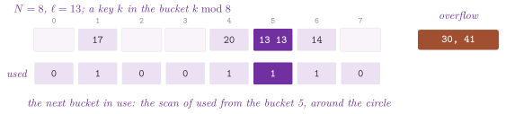
Lemma 9.14. If every key pushed lies in
\([ \ell , \ell + C ]\) with \(C < N\), the overflow is never used, two keys in
one bucket are equal, and the least key is in the first bucket in use from
that of \(\ell\) around the circle; push() then takes \(O( 1 )\) time and
pop() \(O( 1 + N / 64 )\).
Proof. Since \(\ell\) never decreases, the keys in the queue lie in \([ \ell , \ell + N )\). The residues modulo \(N\) of these \(N\) consecutive integers are distinct, and come in the order of the keys from the residue of \(\ell\) around the circle. \(\square\)
When the overflow holds a key smaller than the first bucket in use (or the
buckets are empty), its least key becomes \(\ell\). Its items in the new
window then move to the buckets, each once, a bucket of the radix heap at a
time (RadixHeap::extractBelow(), whose pseudocode follows). Thus a key
pushed far beyond the window costs its moves in the radix heap and one
move into the window. In this way, the scan by words replaces the scan of the buckets one by one
of the original queue, \(O( 1 + C )\), and window() gives \(N\)
(Cherkassky, Goldberg and Radzik 1996
compare these queues for the shortest paths).
BucketQueue< T , K > applies the scan of Dial to two keys: the first, \(f\),
orders the items, and the second, \(g\), breaks the ties towards the largest,
the last item pushed first among equal pairs, which is the order of the search
A* (least \(f\), ties towards the deeper nodes). It is the two-level queue of
the search code of Burns, Hatem, Leighton and Ruml
2012, with no monotonicity required. Its
outer level is a vector of layers indexed by \(f\), scanned forward from a
lazy least \(f\) that only moves forward between two pushes of a smaller \(f\). A
layer, i.e., the items of one \(f\), keeps a LIFO list per \(g\) in one of two
ways (Figure 9.17). The lists of \(g < D\)
(\(D = 256\)) are dense: an array of heads indexed by \(g\), the first \(S = 4\)
in the layer itself and the others in a vector, scanned backward from a bound
that only moves down between two pushes of a larger \(g\). The lists of
\(g \ge D\) are runs while they are at most \(R = 64\): a vector of pairs
\(( g , h )\), \(h\) the head of the list of \(g\), sorted by increasing \(g\), whose
last pair is the top of the layer. A push of any \(g \ge D\) (new or not) into a
layer of \(R\) runs turns the layer dense on all its \(g\), by moving the heads of
the runs (not the items) into an array as long as the largest \(g\). The layer
stays dense until it empties; it then frees the array and is sparse again.
The order among the items of one \(f\) is a policy, the third parameter of
BucketQueue< T , K , Tie > (Ties in the class). LargestSecondKey, the
default, is the order above, while LeastSecondKey takes the least \(g\) first,
and among equal pairs the last item pushed, i.e., the lexicographic order of
the pairs \(( f , g )\), which is that of the keys \(( k_1 , k_2 )\) of LPA*
(Koenig, Likhachev and Furcy 2004), \(k_1\)
the estimate of the cost through a node and \(k_2\) its cost from the start. The
two policies are mirror images: with the least \(g\) first, the bound of the
dense lists is scanned forward and moves only up between two pushes of a
smaller \(g\), the runs are kept by decreasing \(g\), so that their last one is
still the top, and a layer gives its dense lists, all of \(g < D\) while it has
runs, before its runs. The costs of Lemma 9.15 hold
for both, and the default compiles to the same code as before the policy
existed (test engineered.bucket-queue-lexicographic).
The public members of BucketQueue are the following:
// declarations of <ADS/priority/BucketQueue.h>
template< class T , std::integral K = int , BucketTie Tie = LargestSecondKey >
class BucketQueue
{
 public:
 struct Entry
 {
  T item;
  K f , g;
  };
 void push( const T & x , K f , K g );
 const T & top( void );
 K topF( void );
 K topG( void );
 T pop( void );
 Entry popEntry( void );
 struct TopEntry
 {
  const T & item;
  K f , g;
  };
 TopEntry topEntry( void );
 bool empty( void ) const;
 std::size_t size( void ) const;
 void clear( void );
 };
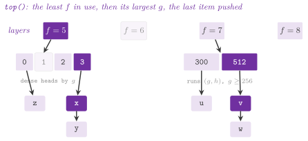
Lemma 9.15. Between two times at which a layer is empty, let it receive \(m\) pushes and as many pops, and let \(u\) be the sum, over the pushes into its dense lists, of the amount by which each push raises the bound of the scan (\(g\) minus the bound, when positive, the bound being 0 at a push into the empty layer). Then the operations on the layer cost \(O( m + u )\) if no push of a \(g \ge D\) meets the layer with \(R\) runs (which holds, e.g., when its items have fewer than \(R\) distinct \(g \ge D\)), and \(O( m + u + G )\) otherwise, \(G\) the largest \(g\) pushed into it. Furthermore, \(u < D\) in the first case, and \(u \le G\) in the second, when all the pushes come before all the pops; with the pushes and the pops interleaved, \(u\) may reach \(\Theta( m D )\).
Proof. A push to the runs costs \(O( 1 )\) when its \(g\) is not below the last, and \(O( \log R + R ) = O( 1 )\) otherwise, since \(R\) is a constant and the shift moves at most \(R\) runs; a pop takes the head of the last run in \(O( 1 )\). A step of the scan of the dense lists lowers the bound by one, the bound is never negative, and only a push raises it; hence the steps are at most \(u\), and the rest of a push or a pop on the dense lists costs \(O( 1 )\). The conversion and the array that follows it cost \(\Theta( G )\) more, to allocate and to set, and the conversion needs \(R\) runs, i.e., more than \(R\) pushes. When the pushes come before the pops, the bound only grows while they last, from 0 to the largest \(g\) of the dense lists, which is below \(D\) without conversion and at most \(G\) with it, and \(u\) is that largest \(g\). Finally, with \(m / 2\) items of \(g = 0\) pushed first, each round of a push of \(g = D - 1\) and two pops raises the bound by \(D - 1\) and costs a scan of \(D - 1\) steps at its second pop, which gives \(\Theta( m D )\) over \(m / 2\) rounds. \(\square\)
In particular, a layer that is filled and then emptied costs \(O( m + D )\),
or \(O( m + D + G )\) after a conversion, i.e., \(O( 1 + ( D + G ) / R )\) per
push in the second case, which is the use of the least layer by a search
A* that pops the nodes of one \(f\) before it pushes any other of that \(f\);
the queue gives no such bound when it alternates pushes of large \(g\) with
pops in the same layer. A dense array by itself would cost \(\Theta( G )\) at each filling of a layer,
even of one item, which is the case of the least layer of a search whose
nodes come in small batches. A binary heap per layer would cost
\(O( \log m )\) per operation, more than the dense lists on a layer of many
items, and would lose the order of the lists, which the view walks (the
layers by increasing \(f\), then the lists by decreasing \(g\), each from its
last item). The items lie in one vector of cells (the Cell, with the
index of the next cell of its list). Freed by the pops, the cells form a
list that the pushes take first, and no operation calls the allocator once
the vector has grown to the largest size of the queue; the vectors of runs
of the layers that empty are kept for the next layers that need one. The
memory is
\(F\) the largest \(f\) pushed, \(H_f\) the heads of the layer \(f\) while it is in
use (at most \(D\) if it is sparse, its largest \(g\) if it is dense) and \(L\)
the most layers that had runs at the same time. topF() and topG() read
the keys of the top, topEntry() returns the top with both keys as a
TopEntry, whose item is a reference into the queue valid up to its next
change, and popEntry() removes the top and returns it with both keys as
an Entry; both find the top once instead of three times (tests
engineered.bucket-queue, engineered.bucket-queue-sparse and
heaps.bucket-queue-cells).
The outer level adds the scan for the least \(f\), which a bound of the same
kind covers. Let \(\varphi\) be the least \(f\) known to the queue: a push sets
it to its \(f\) when the queue is empty or when \(f < \varphi\), and top()
and pop() move it forward to the first layer in use.
Lemma 9.16. Over any sequence of operations, the scans of the outer level make at most \(F + \sum ( \varphi - f )\) steps, \(F\) the largest \(f\) pushed and the sum over the pushes of an \(f < \varphi\); hence at most \(2 F\) steps in all when no push has an \(f\) smaller than the last \(f\) popped.
Proof. A step of a scan raises \(\varphi\) by 1, a push lowers it by \(\varphi - f\) when \(f < \varphi\) and otherwise leaves it or, into an empty queue, raises it, and \(\varphi\) stays between 0 and \(F\), since a scan stops at a layer in use. The steps are thus at most \(F\) plus the total of the lowerings. A pop leaves \(\varphi\) at the \(f\) that it popped, and pushes only lower it; hence, when no push has an \(f\) smaller than the last \(f\) popped, no push after the first pop lowers \(\varphi\), and those before it lower it by at most \(F\) in all, from the \(f\) of the first push down to the least \(f\) pushed. \(\square\)
In the search A* with a consistent estimate, whose pops come by nondecreasing \(f\) and whose pushes are not below the \(f\) of the node expanded, the outer level thus costs \(O( F )\) in all, i.e., \(O( 1 )\) amortized per operation when the operations are \(\Omega( F )\).
BucketHeap< E , C > puts a BucketQueue behind the interface of a heap
of pairs \(( k , x )\), whose key \(k\) of 64 bits is made by packFG( f , g )
from two keys of 32 bits: \(f\) in the high half and the complement of \(g\) in
the low one, so that the keys under std::less come by least \(f\) and then
by largest \(g\), the order of LargestSecondKey, and keyF() and keyG()
give the two keys back. The queue keeps the items with their \(f\) and \(g\),
and the pair is made again when it comes out. It is the inner queue of a
MultiQueue over such keys (§24.9), whose
pushes and pops then take \(O( 1 )\) amortized time with bounded keys, where
those of a heap take \(O( \log m )\) (test
engineered_queues.multi-queue-buckets).
9.10 Double-ended queues¶
A double-ended priority queue has both the best and the worst item at hand,
and removes either in logarithmic time, which a heap cannot do since its worst
item may be any of its leaves. MinMaxHeap.h has two realizations of plain
items ordered by better(), with push(), min(), max(), popMin() and
popMax(), besides empty(), size(), reserve( n ) and clear().
MinMaxHeap< T , Better > is the min-max heap of Atkinson, Sack, Santoro and
Strothotte 1986: a binary heap in a
vector whose levels alternate, a node of an even level (the root's) being not
worse than any item of its subtree and a node of an odd level not better
(Figure 9.18). Hence the best item is the root, and
the worst is the worse of its children, or the root if it is alone. An item
pushed is swapped at most once with its parent, to reach a level of the right
kind, and then moved up by its grandparents. An item moved down from the root
(or from the child that held the worst) is compared with its up to 2 children
and 4 grandchildren. When it lands on a grandchild, it is swapped with its
parent there if this parent, of the other kind, is now out of order.
The public members of MinMaxHeap are the following:
// declarations of <ADS/priority/MinMaxHeap.h>
template< class T , class Better = std::less< T > >
class MinMaxHeap
{
 public:
 explicit MinMaxHeap( Better better = Better() );
 void push( const T & x );
 const T & min( void ) const;
 const T & max( void ) const;
 T popMin( void );
 T popMax( void );
 bool empty( void ) const;
 std::size_t size( void ) const;
 void reserve( std::size_t n );
 void clear( void );
 };
IntervalHeap< T , Better > is the interval heap of van Leeuwen and Wood
1993: the items two by two in the nodes
of a complete binary tree, each node an interval
\([ \mathit{lo} , \mathit{hi} ]\) with
where \(\preceq\) is the order of better(). The \(\mathit{lo}\) of the nodes
form a heap for the best item, the \(\mathit{hi}\) a heap for the worst, and
the root holds both ends. A walk of either kind costs at most two
comparisons per level, on a tree of half the height of a binary heap, with
the two items of a node in one line of the cache.
The public members of IntervalHeap are the following:
// declarations of <ADS/priority/MinMaxHeap.h>
template< class T , class Better = std::less< T > >
class IntervalHeap
{
 public:
 explicit IntervalHeap( Better better = Better() );
 void push( const T & x );
 const T & min( void ) const;
 const T & max( void ) const;
 T popMin( void );
 T popMax( void );
 bool empty( void ) const;
 std::size_t size( void ) const;
 void reserve( std::size_t n );
 void clear( void );
 };
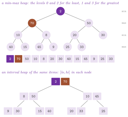
Lemma 9.17. In a min-max heap the best item is the root and the worst is the worse of the children of the root; in an interval heap both are in the root. A push makes \(O( \log n )\) comparisons in either heap, and so does a removal of either end.
Proof. In a min-max heap each item is in the subtree of the root, whose level is even, and in the subtree of one of the children of the root, whose level is odd. In an interval heap, (9.8) gives by induction \(\mathit{lo}( \mathrm{root} ) \preceq x \preceq \mathit{hi}( \mathrm{root} )\) for each item \(x\). Each walk visits one node per level, or per two levels with the grandchildren, and looks at a constant number of items there. \(\square\)
In both heaps, a run of removals with no push in between sorts the items
once it is as long as \(\max\{ 64 , n / 8 \}\) (by the radix sort of
chapter 12 for the numbers and the pairs of numbers in
the order of std::less or std::greater, through OrderKey.h). Then the
rest of the run takes them from the two ends of the sorted array in
\(O( 1 )\) each, as a balanced tree would. In turn, the next push makes the array a
heap again in \(O( n )\) time: an interval heap straight from the sorted
items, the node \(j\) holding the \(j\)-th best and the \(j\)-th worst, and a
min-max heap by the construction from the bottom up of the paper.
Lemma 9.18. With the sort of the runs of removals, each removal of a min-max heap or of an interval heap costs \(O( \log n )\) amortized.
Proof. A sort costs \(O( n \log n )\), and the construction of a heap that follows it \(O( n )\). We charge both to the removals of the run that caused the sort, which are at least \(n / 8\), i.e., \(O( \log n )\) each. \(\square\)
The tests heaps.double-ended-heaps and heaps.large-heap-audits check
both heaps against a multiset, through runs of removals on sorted items and
the pushes that make them heaps again.
These heaps (and the sequence heap of §9.12) take
the keys of the numbers from OrderKey.h, whose functions and constants lie
in the namespace ADS::detail, since they serve the realizations and are not
meant for the user. There orderKey( x ) maps a number of at most 8 bytes, or
a pair of numbers of at most 8 bytes in all (IsNumberPair, the concept
OrderKeyed), to an unsigned word whose order is that of the items. For a
number, it is the key of the radix sort: the sign bit flipped for a signed
integer, all the bits flipped for a negative floating point number and the
sign bit otherwise. For a pair, it is the key of its first item followed by
that of the second, and orderKeyBy< C >( x ) complements it for
std::greater (the constants kAscending, kDescending and kKeyed of the
header tell, at compile time, whether an order is one of the two and has
keys). A comparison of two keys is then a comparison of two words, which the
compiler makes with no jump (a comparison of two pairs takes two), and the
keys give the radix sort its digits. Two items equal in the order have the
same key, but for the floating point zeros, \(-0\) coming before \(+0\), which
only breaks a tie; a NaN, which has no place in the order, has one among the
keys.
9.11 Merging sorted sequences¶
The merge of \(k\) sorted sequences extracts at each step the least of their
first items. A heap of the \(k\) first items does it with a pop() and a
push(), up to \(3 \lfloor \log_2 k \rfloor\) comparisons, or with a
replacement of its top in one walk down, up to \(2 \lfloor \log_2 k \rfloor\),
as in Morin 2013, exercise 10.11
(§9.4). The tree of losers of a tournament (Knuth
1998, §5.4.1) does it with half as many.
LoserTree< T , C > has the \(k\) players (the sequences) as the leaves of a
complete binary tree laid out as a heap: the leaf of the player \(i\) is the
node \(k + i\), and the parent of the node \(v\) is \(\lfloor v / 2 \rfloor\). Each
internal node keeps the loser of the match played there, and the node 0 the
overall winner, i.e., the player of least key and, among equal keys, of least
index. A merge through the tree is thus stable; a player that ran out loses
all its matches (Figure 9.19).
The public members of LoserTree are the following:
// declarations of <ADS/priority/LoserTree.h>
template< class T , class C = std::less<> >
class LoserTree
{
 public:
 explicit LoserTree( std::vector< std::optional< T > > keys , C less = C() );
 std::size_t players( void ) const;
 bool empty( void ) const;
 std::size_t winner( void ) const;
 const T & top( void ) const;
 void replace( std::optional< T > key );
 };
When the winner gets its next key, or runs out, replace() replays only
the matches on the path from its leaf to the root, each against the loser
stored there.
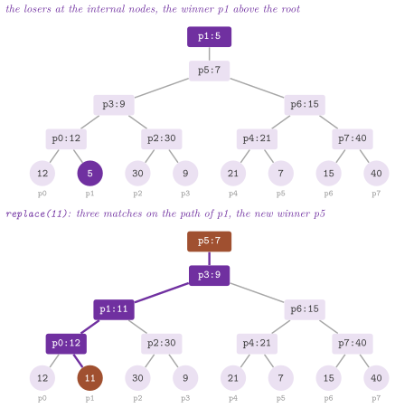
Lemma 9.19. A replay makes
\(\lfloor \log_2 k \rfloor\) or \(\lceil \log_2 k \rceil\) comparisons, and the
merge of \(n\) items in all through kWayMerge() makes at most
comparisons, the term \(k\) for the construction.
Proof. Its construction plays each of the \(k - 1\) matches once, after which each internal node holds the loser of the match between the winners of its two subtrees, and the node 0 the winner. When the winner changes its key, only the matches on its path can change. At each node of the path the new candidate meets the winner of the other subtree, which did not change, and this winner is the loser stored there; the winner of the match goes up and the loser stays. Also, the path from a leaf \(k + i\) to the root has \(\lfloor \log_2( k + i ) \rfloor\) internal nodes, i.e., \(\lfloor \log_2 k \rfloor\) or \(\lceil \log_2 k \rceil\), and a match on equal keys is decided by the indices with the same single call of the order. \(\square\)
players() gives \(k\), empty() tells whether all the players have run
out, winner() the index of the winner and top() its key. In external memory the same merge, fed by one block per sequence, is
the step of the multiway mergesort (cf.
chapter 23), and the tests
pearls_io.ch5.loser-tree and pearls_io.ch5.merge-sorts follow the
notes of Ferragina 2023, chapter 5,
which use a heap of \(k\) pairs for the same purpose.
MultiwayMerge.h engineers the merge in two ways. FlatLoserTree< T , C >
keeps in each of its \(K - 1\) internal nodes (\(K\) the power of two not below
\(k\)) the key of the loser together with its source, instead of the index of
the player. A replay thus reads only the array of the tree, and never the
sequence of a loser. A key of at most 16 bytes copied as bytes is kept by
value, a larger one by its address. On integers in their natural order (the
constant kNaturalOrder) a match compares the pairs (key, source) by two
flags of the keys and one of the sources, an exhausted source having the largest key and its index
with the highest bit set. Its matches are then made of flags, and the swaps of
the winner with the loser of a node of masks, with no jump. This matters since
the matches of a merge of random keys are won by either side with probability
\(1 / 2\), which a branch predicts wrongly half of the time. The sources are
given by start( s , x ) before build(), and replaceTop( x ) and
exhaustTop() replay the path of the winner,
\(\log_2 K = \lceil \log_2 k \rceil\) matches; sources(), empty(),
winner() and top() read the tree. As in LoserTree, equal keys are won by
the lower source, and a merge through the tree is stable.
The public members of FlatLoserTree are the following:
// declarations of <ADS/priority/MultiwayMerge.h>
template< class T , class C = std::less<> >
class FlatLoserTree
{
 public:
 explicit FlatLoserTree( std::size_t k , C less = C() );
 std::size_t sources( void ) const;
 void start( std::size_t s , const T & x );
 void build( void );
 bool empty( void ) const;
 std::size_t winner( void ) const;
 const T & top( void ) const;
 void replaceTop( const T & x );
 void exhaustTop( void );
 };
multiwayMerge( R , out , less ) merges \(k\) sorted ranges into an output
iterator. On contiguous ranges of items copied as bytes it builds a tree of
binary mergers (the halves of the sources below each node), with a buffer of 4
KiB at each internal node, filled lazily. A node merges its two children into
its buffer when the buffer runs out, a child being refilled when it runs out
in turn. This is the \(k\)-merger of the cache-oblivious funnelsort of Frigo,
Leiserson, Prokop and Ramachandran 2012,
made of binary mergers as Brodal, Fagerberg and Vinther
2008 engineered it. A merge of two goes by
stretches as long as the least of the room left in its two inputs and in its
output, \(\min\{ | X | , | Y | , | O | \}\). Since each step takes one item from
one input, the steps of a stretch check no end. Each step is a comparison, a
store of the item picked by a mask and the advance of an input by the flag,
with no jump.
An item climbs \(\lceil \log_2 k \rceil\) mergers, \(O( n \log k )\) time in
all with the constant of a merge of two sequences, and the buffers take
\(4 ( k - 1 )\) KiB, which fit in the cache for the fan-ins of the external
sorts. Items of more than 16 bytes in 3 or 4 ranges are merged by
computing at each step the least head of each pair and the least of the
two, with no jump, and an item is copied once. Two ranges are merged by
the step with no jump, one range is copied, and the other iterators and
types go through FlatLoserTree, in \(O( n \log k + k )\) time. Such a tree of
losers with the keys in the nodes is that of Knuth 1998,
§5.4.1, whose cache behavior Sanders
2000 analyzed. Also the multiway merge of
the MCSTL (Singler, Sanders and Putze
2007) has the same tree, with branches
on the matches (tests engineered_pearls.flat-loser-tree,
engineered_pearls.multiway-merge and
engineered_pearls.multiway-merge-large).
9.12 A priority queue for the caches¶
In the model of the cache, with \(M\) items in the cache and \(B\) in a block (a
line or a page), a heap of \(n \gg M\) items misses the cache at almost each
level of a walk below the levels that fit, i.e., \(\Theta( \log( n / M ) )\)
times per operation, and the misses (not the comparisons) then typically
dominate its cost. The sequence heap of Sanders
2000, SequenceHeap< T , Better >, keeps
instead its items in sorted sequences, merged in large batches, so that its
memory is read and written in order (Figure 9.20).
New items go to an insertion heap \(I\) of at most \(m\) items, small enough to
stay in the first level of the cache, and the best items wait, sorted, in a
deletion buffer \(D\). When \(I\) is full, its items are sorted into a sequence
that joins the group 1. In general, the group \(i\) holds up to \(k\) sorted
sequences of at most \(m k^{i - 1}\) items each, and a buffer of its best items,
refilled by merging its sequences; when a group is full, its sequences and the
buffer of the group \(i + 1\) are merged into one sequence that joins the group
\(i + 1\). Finally, the deletion buffer is refilled by merging the buffers of
the groups.
The public members of SequenceHeap are the following:
// declarations of <ADS/priority/SequenceHeap.h>
template< class T , class Better = std::less< T > >
class SequenceHeap
{
 public:
 explicit SequenceHeap( Better better = Better() );
 void push( const T & x );
 const T & top( void );
 T pop( void );
 bool empty( void ) const;
 std::size_t size( void ) const;
 void clear( void );
 };
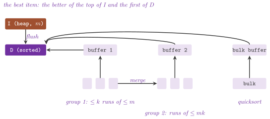
Two invariants hold: the deletion buffer holds items not worse than any other item but those of the insertion heap, and the buffer of a group holds items not worse than those of the sequences of its group. To keep them, a new sequence from the insertion heap is first merged with the deletion buffer and with the buffer of the group 1, which keep the best items of the three. If its best item is not better than the last items of both, however, it joins the group with no merge. The best item is then the better of the top of the insertion heap and of the first item of the deletion buffer.
Theorem 9.4. (Sanders 2000, Theorem
1.) Let a sequence heap have an
insertion heap of \(m\) items, groups of at most \(k\) sequences, the group \(i\)
with sequences of at most \(m k^{i - 1}\) items, and the two invariants
above, and let its merges be made by trees of losers that read and write
their sequences in order. With \(R = \lceil \log_k( n / m ) \rceil\) groups,
push() and pop() then make \(O( \log m + R \log k ) = O( \log n )\)
amortized comparisons, and with \(m = \Theta( M )\) and
\(k = \Theta( M / B )\) they cause
amortized misses of the cache per item.
We do not reproduce the proof, whose amortization over the merges of the full groups charges to each item the merges of the groups that it crosses and the refills of their buffers. The hypotheses hold for the code as far as the scheme of the paper goes: the sizes of the groups and the two invariants are those above, and the merges are those of the trees of losers of §9.11, which read and write in order. However, the theorem covers neither the compaction of a full group that is half empty, which the code adds and for which we give no bound, nor the bulk of the pushes into an empty heap, whose incremental quicksort has the bound of Navarro and Paredes given below.
The bound (9.10) is that of the sorting in external memory divided by the
items. In the code \(m = 4096\) (the public constant M), and the insertion heap of pairs of two
words fills the first level of the cache and its sequences the second;
also, \(k = 16\) (the constant K). Its merges are made by trees of losers whose matches are
decided by conditional moves, and the numbers and the pairs of numbers are
compared in the merges by their keys of OrderKey.h, and their sequences
sorted by the radix sort. Its insertion heap is 4-ary and compares by
better(), whose jumps the processor predicts ahead, where the
conditional moves would chain the loads of the walk down. A group that is full but holds at most
half of its room is first compacted into fewer full sequences instead of
being pushed to the next group.
The pushes into an empty heap, before any top() or pop(), go to a bulk,
an array in the order of the pushes, where an insertion is a store. The
first look at a large bulk finds its best item by a scan, which serves a
top() or a pop() after a load with one read per item; at the next one
the bulk becomes an incremental quicksort (Paredes and Navarro
2006), which splits the array by the
median of three into the better items, the pivot and the others, keeps
the places of the pivots on a stack and splits again only the leftmost
part, until it holds at most \(m\) items, which are sorted into the buffer
of the bulk, one more source of the deletion buffer. This costs
\(O( n + j \log j )\) expected time for the \(j\) best items of \(n\), and
\(O( \log n )\) amortized per extraction (Navarro and Paredes
2010). The items equal to a pivot that
has no better one are split off with it, and many equal keys thus cost no
quadratic time. A small bulk goes to the insertion heap, made a heap only
when a top() or a pop() needs it (test heaps.sequence-heap).
9.13 The realizations compared¶
The choice among the realizations depends first on the operations that a
computation needs, and only then on their constants. A queue that is only
pushed and popped, with "small" items that carry their keys, is typically
best served by DaryHeap with \(D = 4\) (Lemma 9.5),
or, when it holds many more items than the cache, by SequenceHeap
(Theorem 9.4); the lazy deletion makes either one
serve the algorithms that would decrease a key. When the items are the
nodes of a graph and the decreases are real, IndexedDaryHeap keeps the
keys in the heap and the places in a vector, and is usually preferable to
the heaps with pointers, whose decrease() is "cheaper" in the amortized
sense but whose nodes are scattered in memory: among those, the pairing
heap is typically faster than the Fibonacci heap in practice (Stasko and
Vitter 1987; Larkin, Sen and Tarjan
2014), although only the latter has the
bound of Theorem 9.3. A merge of two queues calls
for MeldableHeap, the only realization whose merge is logarithmic, and
the extraction of both ends for IntervalHeap, usually faster than
MinMaxHeap in practice, since its tree is half as deep and the two
items of a node share a line of the cache. When the keys are small
integers and the queue is monotone, DialQueue and RadixHeap find the
least key by the position of the keys, without comparisons, and
BucketQueue does it on the two keys of a search A*. Finally, the lists and the
tree of §9.2 are there for teaching and for the
few cases (a handful of items, or the need for the items in order) where
their costs do not matter.
A comparison of the times of these realizations belongs to the campaign of
measurements on an idle machine of appendix B, and we give none here. We
only remark that the asymptotic bounds of Table 9.1
are a poor guide between the heaps with logarithmic operations, whose
differences come from the misses of the cache, the mispredicted branches
and the calls of the allocator, which the engineered variants of the
chapter address one by one: the plain items and the hole of DaryHeap, the
pools of the heaps with handles, the keys without jumps of OrderKey.h
and of FlatLoserTree, and the sequences in order of SequenceHeap.
9.14 Discussion and references¶
The binary heap is due to Williams 1964,
as the structure of heapsort, and its construction in linear time to
Floyd 1964; the representation of a
complete tree in a vector goes back to Eytzinger
1590, as Morin 2013,
§10.3 recalls. The \(d\)-ary heap and the
choice of \(d\) for the shortest paths are due to Johnson
1975, the walk from the bottom up to
Floyd 1964 and Wegener
1993, and the effect of the caches on
the heaps was studied by LaMarca and Ladner
1996 and, with the conclusion that a
4-ary heap of plain items is hard to beat, by Larkin, Sen and Tarjan
2014. Also the randomized meldable heap is
due to Gambin and Malinowski 1998;
other meldable heaps are the leftist heaps (Knuth 1998,
§5.2.3), the binomial queues of
Vuillemin 1978, the skew heaps of
Sleator and Tarjan 1986, and the
Fibonacci and pairing heaps of §9.7 and
§9.8, none of which is as simple as the
randomized one (Morin 2013, §10.3). As for the heaps with decrease-key, the
Fibonacci heap is due to Fredman and Tarjan
1987, the pairing heap to Fredman,
Sedgewick, Sleator and Tarjan 1986,
with the variants and the experiments of Stasko and Vitter
1987, the lower bound of Fredman
1999 and the upper bounds of Iacono
2000, Pettie
2005 and Elmasry
2009. In turn, the monotone queues are due to
Dial 1969 and to Ahuja, Mehlhorn,
Orlin and Tarjan 1990, and were compared
for the shortest paths by Cherkassky, Goldberg and Radzik
1996; the two-level bucket queue
for the search A* is that of Burns et al.
2012. Finally, the double-ended heaps are those of
Atkinson et al. 1986 and of van
Leeuwen and Wood 1993, the tree of
losers is in Knuth 1998, §5.4.1, the
funnel in Frigo et al. 2012 and Brodal
et al. 2008, and the sequence heap in
Sanders 2000, with the incremental
quicksort of Paredes and Navarro 2006;
Sanders et al. 2019, chapter 6 is a
modern survey of most of them. The algorithms on graphs of
chapter 14 take the heaps of this chapter that support
decrease(), and heapsort and the multiway merges
reappear in chapter 12.
9.15 Exercises¶
Each exercise names the test of the library that solves it (run it with
ctest -R <name>). The first eleven are those of Morin 2013,
§10.3, in his order.
- Illustrate the insertion of 7 and then of 3 into the binary heap that
ends Figure 9.3 (Morin 2013, exercise
10.1); the solution is
Figure 9.5. Test:
ods_ints.ods10.1.binary-heap. - Illustrate the next two removals, of 6 and of 8, from the binary heap
that ends Figure 9.4 (Morin 2013, exercise
10.2); the solution is
Figure 9.6. Test:
ods_ints.ods10.1.binary-heap. - Remove the item in the place \(i\) of a binary heap in \(O( \log n )\)
time, and explain why the operation is of little use (Morin 2013,
exercise 10.3;
Lemma 9.7). Test:
ods_ints.ods.ex10.3.remove-place. - Give the places of the parent and of the \(d\) children of the place \(i\)
in the layout of Eytzinger of a complete \(d\)-ary tree (Morin 2013,
exercise 10.4;
Lemma 9.1). Tests:
ods_ints.ods.ex10.3.remove-place,ch10.ex10.5. - Realize the \(d\)-ary heap, analyze its operations and compare it with
the binary heap (Morin 2013, exercise
10.5;
Lemma 9.5). Tests:
ods_ints.ods.ex10.5.dary-heap,ch10.ex10.6. - Illustrate the insertion of 17 and then of 82 into the meldable heap
\(h_1\) of Figure 9.11, with a coin for the
random bits (Morin 2013, exercise 10.6);
a solution is in Figure 9.12. Test:
ods_ints.ods10.2.meldable-heap. - Illustrate the next two removals, of 4 and of 8, from the same heap
(Morin 2013, exercise 10.7); a
solution is in Figure 9.12. Test:
ods_ints.ods10.2.meldable-heap. - Remove the node \(u\) from a meldable heap in \(O( \log n )\) expected time
(Morin 2013, exercise 10.8). Test:
ods_ints.ods10.2.meldable-heap. - Find the second least item of a binary heap and of a meldable heap in
constant time (Morin 2013, exercise
10.9). Tests:
ods_ints.ods.ex10.3.remove-place,ods_ints.ods10.2.meldable-heap. - Find the \(k\)-th least item of a binary heap or of a meldable heap in
\(O( k \log k )\) time, with the help of a second heap (Morin 2013,
exercise 10.10;
Lemma 9.8). Test:
ods_ints.ods.ex10.10.k-smallest. - Merge \(k\) sorted lists of \(n\) items in all into one sorted list in
\(O( n \log k )\) time with a heap (Morin 2013, exercise
10.11); compare with the merge of the
\(k\) lists one after the other, \(O( n k )\). Tests:
ods_ints.ods.ex10.11.k-way-merge,ch10.ex10.3,exam_collezionia.collezioni-10-heap-1-7-2. - Realize the PRIORITYQUEUE on a sorted list, on an unsorted list, on a
balanced search tree and on a heap, and check them against its
axioms (9.1). Tests:
ch10.spec.ListPriorityQueue,ch10.spec.TreePriorityQueue,ch10.spec.HeapPriorityQueue,contract_priority.priority-axioms. - Build the heap of the vector 5, 10, 8, 11, 13, 12, 9, 18, 3, 6 of
Montresor 2025, Figure 10.1,
delete its minimum and insert 4, following the figures of the book.
Test:
ch10.sec10.1.3.heap. - Show that the symmetric visit of a heap is not sorted, and that the
order of \(n\) items cannot be read from a heap in \(O( n )\) time,
although a heap is built in \(O( n )\) (Lemma 9.4).
Test:
ch10.ex10.1. - Write the walk down of a max-heap iteratively, with \(O( 1 )\) extra
space. Test:
ch10.ex10.4. - Give the level of the last place of a ternary heap of \(n\) items, and
check it by the parents of the library. Test:
exam_collezionia.collezioni-10-heap-1-8-2. - Show that the greatest item of a min-heap is in a leaf, and decide
whether a vector is a max-heap. Tests:
exam_collezionia.collezioni-10-heap-1-9,exam_collezionia.collezioni-10-heap-1-10. - Realize the heap on a binary tree with pointers, finding the last leaf
by the bits of \(n\) and by a walk from the previous one
(§9.5). Tests:
beyond.linked-heap,heaps.linked-heap-pool. - Give the items of the heap with handles a pool of their own, so that an
insertion after a deletion calls no allocator. Test:
heaps.heap-priority-queue-pool. - Realize the \(d\)-ary heap of the ids \([ 0 , n )\) with
decrease(),increase(),update()anderase(). Tests:engineered_graph.indexed-dary-heap,engineered_search.indexed-heap-erase. - Keep a frontier by one key and know at each moment the least of a
second key over it. Test:
engineered_search.indexed-heap-pair. - Realize the walk from the bottom up of
pop()and check it againststd::priority_queuefor \(D = 2 , 3 , 4 , 8\). Tests:heaps.dary-heap-bottom-up,engineered.dary-heap. - Realize the Fibonacci heap and use it in the algorithms of Dijkstra and
Prim (Theorem 9.3). Tests:
ch11.sec11.5.fibonacci,ch11.sec11.5.fibonacci-pool,ch14.ex14.4,contract_priority.fibonacci-heap-priority-queue. - Realize the pairing heap with two passes and its auxiliary variant, and
add to it the removal and the raise of any item. Tests:
heaps.pairing-heap,engineered_search.pairing-heap-erase. - Realize the radix heap with digits of \(B\) bits and the queue of Dial
with an overflow, and check that a key below the last one extracted
violates their contracts (Lemma 9.13 and
Lemma 9.14). Tests:
heaps.radix-heap,heaps.dial-queue. - Realize the two-level bucket queue of the search A*, dense for the
small second keys and sparse for the large ones
(Lemma 9.15). Tests:
engineered.bucket-queue,engineered.bucket-queue-sparse,heaps.bucket-queue-cells,contract_priority.bucket-dary-loser. - Realize the min-max heap and the interval heap, with the sort of the
runs of removals (Lemma 9.18), and audit the
order of large heaps in linear total time. Tests:
heaps.double-ended-heaps,heaps.large-heap-audits. - Merge \(k\) sorted runs through a tree of losers with
\(\lceil \log_2 k \rceil\) comparisons per item, stably
(Lemma 9.19), and through the tree with the
keys in its nodes and the funnel of binary mergers. Tests:
pearls_io.ch5.loser-tree,engineered_pearls.flat-loser-tree,engineered_pearls.multiway-merge,engineered_pearls.multiway-merge-large. - Realize the sequence heap of Sanders with the incremental quicksort of
the pushes into an empty heap. Test:
heaps.sequence-heap. - Draw a sample of \(n\) items from a stream of unknown length by a heap of
random keys, and compare it with the reservoir. Test:
pearls_io.ch3.heap-sampling.