16. Geometry¶
[Source: include/ADS/geometry/ConvexHull.h, ClosestPair.h,
IntervalTree.h, RangeTree.h]
We are concerned in this chapter with two problems on a finite set of
points of the plane, the convex hull and the closest pair, and with two
queries on sets that change: which intervals contain a point, and how many
points lie in a rectangle. Both problems rest on one predicate, the
orientation of three points, which is exact on integer coordinates
(§16.1). In §16.2
we compute the convex hull by checking every segment, by the scan of
Graham (a backtracking on a stack), and by an engineered variant that drops
most of the points before sorting them. In
§16.3 the closest pair is found by comparing all
the pairs, by divide and conquer, by a sweep of the plane and by a
randomized grid. Finally, §16.4 answers the two
queries by maps whose nodes keep a summary of their subtree (the augmented
maps of §8.12.6), i.e., the largest right end of the intervals and the
sorted ordinates of the points, respectively. Throughout the chapter \(n\)
is the number of points or intervals of the input, \(h\) the number of
vertices of a hull, \(k\) the number of points that survive a filter (or of
intervals that a query reports), and \(\delta\) the least distance of two
points found so far. In the sets of §1.9,
IntervalTree.h and RangeTree.h are advanced and the other headers of
this chapter are base.
16.1 Points and orientation¶
A point \(p = ( x_p , y_p )\) has integer coordinates (Point of
ConvexHull.h, two long), and the input is a set \(P\) of \(n\) points,
possibly with repetitions. We call orientation of three points \(a\), \(b\),
\(c\) the sign of the cross product
i.e., of twice the signed area of the triangle \(a b c\). It is positive when \(c\) lies to the left of the line from \(a\) to \(b\) (the turn from \(a\) through \(b\) to \(c\) is counterclockwise), negative when \(c\) lies to the right, and 0 when the three points are collinear. Each decision of the algorithms of §16.2 is a sign of (16.1), and each decision of those of §16.3 a comparison of squared distances; hence, all of them are exact as long as the arithmetic does not overflow, which the preconditions of the functions ensure.
Lemma 16.1. If \(| x | \le 10^9\) and \(| y | \le 10^9\) for all the points, then (16.1) and the square \(d^2( p , q ) = ( x_p - x_q )^2 + ( y_p - y_q )^2\) of the distance of two points are computed exactly in signed integers of 64 bits.
Proof. A difference of two coordinates is at most \(2 \cdot 10^9 < 2^{31}\) in absolute value. Each of the two products of (16.1) is thus below \(4 \cdot 10^{18}\), and their difference below \(8 \cdot 10^{18}\), in absolute value; the same bound holds for the sum of two squares. Since \(2^{63} > 9.2 \cdot 10^{18}\), no intermediate result overflows. \(\square\)
The functions convert the coordinates to long long before computing
(16.1), since long has 32 bits on some platforms (Windows among them);
the predicates of this section are declared as
// declarations of <ADS/geometry/ConvexHull.h>
struct Point
{
 long x , y;
 };
long long cross( const Point & a , const Point & b , const Point & c );
bool sameSide( const Point & p1 , const Point & p2 , const Point & p ,
               const Point & q );
double pseudoAngle( long dx , long dy );
Two points \(p\) and \(q\) lie on the same side of the line through \(p_1\) and
\(p_2\) when the two orientations agree in sign, a point on the line counting
on both sides (sameSide(), the procedure of Montresor 2025,
§16.1):
An algorithm that sorts points by angle around a center has to compare the
angles of two vectors, and one can do so without trigonometry, either by the
sign of (16.1) when the two vectors lie in the same half-plane, or by a
value that grows with the angle. pseudoAngle() gives such a value for the
vector \(( \mathit{dx} , \mathit{dy} ) \ne ( 0 , 0 )\): with
\(t = \mathit{dy} / ( | \mathit{dx} | + | \mathit{dy} | )\), it is
and 0 for the null vector, so that the four semi-axes from the positive \(x\) one have the values 0, 1, 2 and 3 (Montresor 2025, exercise 16.1).
Lemma 16.2. The value (16.2) lies in \([ 0 , 4 )\) and is a strictly increasing function of the angle \(\theta \in [ 0 , 2 \pi )\) of the vector, measured counterclockwise from the positive \(x\) axis.
Proof. In each quadrant \(| \mathit{dy} | / ( | \mathit{dx} | + | \mathit{dy} | ) = 1 / ( 1 + | \cot \theta | )\), which grows with \(\theta\) in the first and in the third quadrant and decreases in the second and in the fourth. Thus \(t\) grows from 0 to 1 in the first quadrant, \(2 - t\) grows from 1 to 2 in the second (where \(t\) goes from 1 to 0) and from 2 to 3 in the third (where \(t\) goes from 0 to \(-1\)), and \(4 + t\) grows from 3 towards 4 in the fourth, without reaching it. At the semi-axes the values agree with the limits from both sides, and therefore the function increases on the whole circle. \(\square\)
The function is computed in double, since \(| \mathit{dx} | +
| \mathit{dy} |\) may overflow a long. In floating point, a direction just
below the positive \(x\) axis gives a value \(4 + t\) that would round to 4;
the code returns instead the largest double below 4, which keeps the
value in \([ 0 , 4 )\) at the price of a tie with the directions next to it.
Of course, rounding may tie two directions that differ by less than the
precision of a double in any quadrant, whereas (16.1) is exact; for this
reason the hulls of §16.2 sort by (16.1), and
pseudoAngle() serves the algorithms that need a key of the angle.
16.2 The convex hull¶
A set of the plane is convex if it contains the segment between any two
of its points, and the convex hull of \(P\) is the smallest convex set that
contains \(P\) (the intersection of all the convex sets that contain it). For
a finite \(P\) it is a convex polygon whose vertices are points of \(P\), and
an algorithm of the hull returns these vertices. In ConvexHull.h the
output is unique: a repeated point counts once, a point strictly inside an
edge of the polygon is no vertex, and the vertices come in counterclockwise
order from the lowest one (the rightmost of the lowest ones, on a tie).
With fewer than three distinct points, the output is those points sorted by
\(x\) and then \(y\); when all the points are collinear, it is the two ends of
their segment. All the algorithms below rest on the following
characterization of the edges.
Lemma 16.3. Two distinct points \(p , q \in P\) are consecutive vertices of the hull of \(P\), in counterclockwise order, if and only if
and no point of \(P\) lies on the line through \(p\) and \(q\) outside the segment \(p q\).
Proof. By (16.3) the closed half-plane on the left of the line from \(p\) to \(q\) contains \(P\), and hence its hull; the segment \(p q\) is then on the boundary of the hull, which is traversed counterclockwise from \(p\) to \(q\). On the line, the hull is a segment whose ends are the two points of \(P\) on the line that are farthest apart (the two vertices of the edge), and by the second condition these are \(p\) and \(q\). Conversely, the line through two consecutive vertices supports the hull, with the hull on its left, and no point of \(P\) on it lies beyond the two ends of the edge. \(\square\)
convexHullBrute() checks the two conditions of
Lemma 16.3 on each of the \(n ( n - 1 )\) ordered
pairs of distinct points, with at most \(n\) evaluations of (16.1) per pair, and
sorts by angle the vertices that it finds
(Algorithm 16.1). It costs \(O( n^3 )\) time, and
the tests use it as the reference for the other algorithms. In the code,
the second condition of line 5 is the sign of the scalar product
\(( r - p ) \cdot ( r - q )\), which is positive exactly when a point \(r\) of
the line lies outside the segment.
Algorithm 16.1. The hull by checking every segment (Montresor 2025, §16.1).
16.2.1 The scan of Graham¶
The scan of Graham 1972 avoids the pairs that cannot be edges. Its center is the lowest point \(o\) (the rightmost of the lowest ones), which is a vertex; every other point lies above it or on its left on the same row, at an angle in \(( 0 , \pi ]\) around \(o\), so that the sign of (16.1) orders any two of them. Let \(p_1 , \ldots , p_m\) be the other points sorted by increasing angle around \(o\) (the angles compared by the sign of (16.1), the nearer point first on a tie), where of the points collinear with \(o\) only the farthest one is kept. In this order the scan pushes them on a stack \(S\), with the invariant that after the scan of \(p_i\)
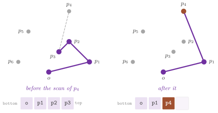
A new point \(p_{i+1}\) is a vertex of the next hull, since it has the largest angle. Instead, the vertex \(t\) on top of \(S\), with \(s\) below it, remains a vertex if and only if the turn from \(s\) through \(t\) to \(p_{i+1}\) is to the left; otherwise \(t\) lies in the triangle \(o \, s \, p_{i+1}\) (or on its side \(s \, p_{i+1}\)). Hence, before pushing \(p_{i+1}\), the scan pops the vertices that make a turn not to the left (Algorithm 16.2), which Montresor 2025, §16.1 presents as a backtrack on the choices made so far. Figure 16.1 shows the scan of a point that pops two vertices.
Algorithm 16.2. The scan of Graham (Graham 1972; Montresor 2025, §16.1).
Lemma 16.4. The scan of Graham returns the vertices of the hull of \(P\) in counterclockwise order from \(o\), in \(O( n \log n )\) time and \(O( n )\) space.
Proof. The invariant (16.4) holds after the scan of \(p_1\), when \(S\) holds \(o\) and \(p_1\). Suppose that it holds after the scan of \(p_i\). A vertex \(t\) popped at line 8 lies in the triangle \(o \, s \, p_{i+1}\), or on its side \(s \, p_{i+1}\), and it is therefore no vertex of the hull of \(\{ o , p_1 , \ldots , p_{i+1} \}\). When the loop stops, the turn from the second vertex of \(S\) through its top to \(p_{i+1}\) is to the left; the vertices left on \(S\), followed by \(p_{i+1}\), form a convex polygon that contains all the points scanned (cf. the triangles above), which is (16.4) after the scan of \(p_{i+1}\). After the last point this is the claim, since the points dropped at line 5 lie inside a segment from \(o\) to a point kept. As for the time, each point is pushed once and popped at most once, and hence lines 7 to 9 cost \(O( n )\); the sort costs \(O( n \log n )\) and dominates. \(\square\)
In the code, the stack is a std::vector. Note that the test \(\le 0\) (instead of \(< 0\)) also pops a vertex collinear
with its neighbors. Together with the order of the ties and with the points
collinear with \(o\) dropped at line 5, it keeps out of the output the points
strictly inside the edges. The output is thus the one fixed above.
No algorithm that decides by comparisons and arithmetic can improve on the bound of Lemma 16.4, as the next theorem shows by reducing sorting to the hull (Preparata and Shamos 1985).
Theorem 16.1. Any algorithm that computes the vertices of the convex hull of \(n\) points in their order on the hull takes \(\Omega( n \log n )\) time in the worst case in the model of the algebraic decision trees.
Proof. Given \(n\) distinct numbers \(a_1 , \ldots , a_n\), the points \(( a_i , a_i^2 )\) lie on the parabola \(y = x^2\), which is convex. Each one is thus a vertex of their hull, and the hull visits them by increasing \(a_i\) from the leftmost one. Building the points and reading the order from the hull costs \(O( n )\); therefore, a hull in \(o( n \log n )\) would sort \(n\) numbers in \(o( n \log n )\), against the lower bound \(\Omega( n \log n )\) of sorting in that model (Ben-Or 1983). \(\square\)
Yao 1981 proves the same bound for the weaker problem of identifying the vertices without their order, in the model of the quadratic decision trees. It is worth noting, however, that Theorem 16.1 concerns the worst case: on the inputs met in practice the hull usually has far fewer vertices than there are points, and an algorithm may exploit this, as the next one does (at least on points spread in a square or in a disk).
16.2.2 The engineered hull¶
convexHull() returns the same polygon as graham(), and it is meant to
be faster on the inputs met in practice by two devices. First, there is the filter
of Akl and Toussaint 1978. Consider the
points of \(P\) that are extreme in the eight directions of the axes and of
the diagonals, i.e., those of largest \(-y\), \(x - y\), \(x\), \(x + y\), \(y\),
\(y - x\), \(-x\) and \(-x - y\) (the first one met, on a tie). They lie on the
boundary of the hull, in this order counterclockwise. Indeed, the points
extreme in a direction form a vertex or an edge of the hull, and these
faces follow one another counterclockwise as the direction turns (a point
extreme in two directions is then extreme in all those between them, which is why a
point repeats only in consecutive places, but for all the points on one
line). Each of them is a vertex unless a tie leaves it inside an edge, as
the first one met may be. Their polygon (the octagon, with fewer than
eight distinct vertices when some of them coincide) is therefore inside the
hull, and a point strictly inside it is no vertex of the hull. One pass over
\(P\) finds the extreme points, and a second one drops each point that lies
strictly to the left of all the edges of the octagon, with at most 8
evaluations of (16.1) per point. When the octagon has fewer than three
distinct vertices the filter drops nothing, and so it does when all of them
lie on one line, since no point is then strictly to the left of an edge
(lines 2 and 3 of Algorithm 16.3).
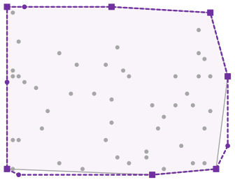
Figure 16.2 shows the filter on random points. On points uniform in a square the extreme points in the diagonal directions tend to the corners and the others to the sides. The octagon thus covers all the points but a fraction that vanishes as \(n\) grows, and the number \(k\) of the points left is \(o( n )\) in expectation. Devroye and Toussaint 1981 show that such a filter followed by any hull in \(O( n \log n )\) takes \(O( n )\) expected time when the density of the points is bounded away from 0 and from \(\infty\) on a rectangle. On points uniform in a disk of radius \(r\), instead, the eight extreme points tend to the points of the circle in the eight directions, and the octagon to the regular octagon inscribed in it, of area \(2 \sqrt{2} \, r^2\); a fraction near \(1 - 2 \sqrt{2} / \pi \approx 0.1\) of the points survives, and \(k = \Theta( n )\). On points near a circle almost all of them survive, and the filter costs one pass over \(P\) with little or no benefit.
Second, sorting the points left by \(x\) and then \(y\), instead of by angle, allows a sort of integer keys. With \(| x | , | y | < 2^{31}\), the key
is an unsigned integer of 64 bits whose order is the lexicographic order of
\(( x_p , y_p )\), and convexHull() sorts the \(k\) keys by sort(), the sort
of ADS that chooses its algorithm (§12.14). On a
vector of at least 512 keys with more than 16 runs and without the vector
registers, sort() takes the radix sort of
§12.10, \(O( k )\) time with at most 8 passes over
bytes. It does not when a sample of 64 keys has at most 16
distinct ones differing in 4 bytes or more; with the registers, it takes
the radix sort only when the keys of the sample differ in one byte.
Otherwise it takes a
quicksort (pattern-defeating, or vectorized when the registers are there)
or the merge of the runs, in \(O( k \log k )\) time in the worst case. On the sorted points, the
monotone chain of Andrew 1979 builds
the lower chain of the hull by the scan of Graham from the leftmost point
to the rightmost one, and the upper chain by the same scan back from the
rightmost point to the leftmost, with the invariant (16.4) on each chain
(Algorithm 16.3). Both scans run on one vector
\(H\) of \(2 k\) places. The upper chain starts from the rightmost point, the
last one that the lower chain pushed, and it never pops it, since the test
of line 8 looks only at the points of the chain at hand (the code keeps on
\(H\) the \(t - 1\) points of the lower chain, the rightmost one included,
while it scans the upper one).
Algorithm 16.3. The engineered hull: the filter of Akl and Toussaint 1978, the sort of the integer keys, and the monotone chain of Andrew 1979.
Lemma 16.5. convexHull() returns the
output of graham() in \(O( n + k \log k )\) time, where \(k \le n\) is the
number of points that are not strictly inside the octagon, and in
\(O( n + k )\) time, hence \(O( n )\), when sort() takes the radix sort.
Proof. By the remark above, the filter drops no vertex of the hull, and
the hull of the points left is thus the hull of \(P\). By the argument of
Lemma 16.4, with the abscissa in place of the
angle, the lower chain is the lower boundary of the hull, and similarly for
the upper chain. The two chains share their ends; line 11 drops the copy
of the leftmost point, and the rotation of line 12 starts the output where
graham() starts it. As for the time, the two passes of the filter cost
\(O( n )\), and the sort \(O( k \log k )\) in the worst case and \(O( k )\) when
it is the radix sort. The removal of the repetitions costs \(O( k )\), and so
do the two scans, since each point is pushed at most twice and popped at
most as many times. \(\square\)
On points uniform in a square, \(k = o( n )\) in expectation, and the bound of
Devroye and Toussaint 1981 gives
\(O( n )\) expected time whichever algorithm sort() takes. We remark that
the bound \(O( n )\) of the radix sort does not contradict
Theorem 16.1, since the radix sort reads the
bytes of the coordinates, an operation that the algebraic decision trees do
not have. Table 16.1 summarizes the three
algorithms.
Table 16.1. The algorithms of the convex
hull in ConvexHull.h; \(k\) is the number of points that survive the
filter of the octagon.
| Function | Algorithm | Time | Source |
|---|---|---|---|
convexHullBrute() |
every segment checked by (16.3) | \(O( n^3 )\) | Montresor 2025, §16.1 |
graham() |
sort by angle, scan with a stack | \(O( n \log n )\) | Graham 1972 |
convexHull() |
octagon, sort of the keys, monotone chain | \(O( n + k \log k )\), \(O( n + k )\) by the radix sort; \(O( n )\) expected on points uniform in a square | Akl and Toussaint 1978, Andrew 1979 |
The three functions take the points by value (or by reference, when they do not sort them in place) and return the vertices in the order fixed at the start of this section, e.g., the 9 vertices of Figure 16.2 from \(( 27 , 1 )\):
// declarations of <ADS/geometry/ConvexHull.h>
std::vector< Point > convexHullBrute( std::vector< Point > P );
std::vector< Point > graham( std::vector< Point > P );
std::vector< Point > convexHull( const std::vector< Point > & P );
16.3 The closest pair¶
A closest pair of \(P\), \(n \ge 2\), is a pair of points at the least
Euclidean distance \(d( p , q )\), the two points being at distinct places of
the input (two repeated points are thus a pair at distance 0). The
functions of ClosestPair.h return the two places \(i < j\) and the square
\(d^2\) of the distance (squaredDistance()), an exact integer by
Lemma 16.1. No square root is ever taken,
since \(d( p , q ) < \delta\) if and only if \(d^2( p , q ) < \delta^2\).
Comparing all the pairs costs \(\Theta( n^2 )\) (closestPairBrute(), which
returns the first pair of the least distance in the order of its loops;
when several pairs tie, it is not always the pair of closestPair()):
16.3.1 Divide and conquer¶
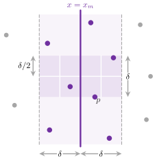
The algorithm of Shamos and Hoey 1975 sorts the points by \(x\) once and splits them at the median abscissa \(x_m\) into two halves, of \(\lfloor n / 2 \rfloor\) and \(\lceil n / 2 \rceil\) points. It solves the two halves recursively, and then looks for a closer pair with one point in each half; this search is linear by the following property (Figure 16.3).
Lemma 16.6. Let the points of each half be at mutual distance at least \(\delta > 0\). Then a pair closer than \(\delta\) with one point in each half has both points in the strip \(| x - x_m | < \delta\). Furthermore, if the points of the strip are sorted by \(y\), each one has at most 7 others of the strip after it whose ordinate exceeds its own by less than \(\delta\).
Proof. A point farther than \(\delta\) from the line \(x = x_m\) is farther than \(\delta\) from every point on the other side. Now let \(p\) be a point of the strip; every point of the strip that follows \(p\) by less than \(\delta\) in ordinate lies in the rectangle \([ x_m - \delta , x_m + \delta ] \times [ y_p , y_p + \delta ]\). Cut it into 8 squares of side \(\delta / 2\), four on each side of the line, whose diameter is \(\delta / \sqrt{2} < \delta\). The points of the left half have \(x \le x_m\), and those of the right half \(x \ge x_m\); hence, a square on the left of the line holds at most one point of the left half, and similarly on the right. Thus the rectangle holds at most 8 points, \(p\) included. \(\square\)
The recursion returns each range sorted by \(y\), merging the two halves as mergesort does, so that the strip comes out in order of \(y\) in linear time; a range of at most 3 points is solved by comparing its pairs (Algorithm 16.4). In the code, a range is a range of a vector \(I\) of the places of the points, sorted by \(x\) at the start, and the merge goes through a buffer \(B\) of \(n\) places, which also holds the strip. Each point of the strip is then compared with the next ones, until their difference in \(y\) reaches the current \(\delta\) (lines 7 to 11).
Algorithm 16.4. The closest pair by divide and conquer (Shamos and Hoey 1975).
Theorem 16.2. closestPair() returns a
closest pair of \(P\) in \(O( n \log n )\) time and \(O( n )\) space.
Proof. We show, by induction on the size of the range, that \(\delta^2\) is at most the least squared distance of two points of the range when the call ends. This is clear in the base case, which compares all the pairs. Otherwise, the two calls on the halves make \(\delta\) at most the least distance within each half, and by Lemma 16.6 a crossing pair closer than \(\delta\) has both points in the strip, at most 7 places apart in its order by \(y\). There the loop of lines 8 to 11 compares it, since the loop stops only at a pair whose difference in \(y\) is not below \(\delta\) (and the later pairs are farther still). As for the time, the strip costs \(O( n )\), with at most 7 comparisons per point, and so does the merge; hence
to which the initial sort by \(x\) adds \(O( n \log n )\). \(\square\)
The bound (16.6) is optimal in the model of the algebraic decision trees. Indeed, \(n\) numbers \(a_1 , \ldots , a_n\) are distinct if and only if the closest pair of the points \(( a_i , 0 )\) is at a positive distance, and deciding the distinctness of \(n\) numbers takes \(\Omega( n \log n )\) time in that model (Ben-Or 1983). Randomized algorithms escape the bound by the floor function, which the model does not have. Rabin 1976 first solved the problem in \(O( n )\) expected time, with a grid whose side is estimated on a sample; the sieve of Khuller and Matias 1995 and the incremental grid of Golin et al. 1995 reach the same bound with simpler arguments.
16.3.2 The sweep and the randomized grid¶
closestPairSweep() returns a pair at the least distance (not necessarily
the one of closestPair(), when several pairs tie), and it is designed for
the usual inputs. It is the sweep of the plane of Hinrichs, Nievergelt and
Schorn 1988, without their balanced
tree. The points, made keys (16.5), are sorted by sort(), in \(O( n )\) time
when it takes the radix sort and in \(O( n \log n )\) otherwise (cf.
§16.2.2); then each one is compared with the points before it in the order, from the
nearest one backwards, until their difference in \(x\) reaches the current
\(\delta\) (Algorithm 16.5). Since the points of
one abscissa (a column) are sorted by \(y\), a point of the same column that
is not closer than \(\delta\) in \(y\) ends the scan of the column. The scan
then jumps to the column before (line 8).
Lemma 16.7. If the budget does not run out, \(\mathrm{sweep}()\) of Algorithm 16.5 returns a closest pair of \(P\).
Proof. Let \(( v^* , u^* )\), \(v^* < u^*\) in the order of \(K\), be a closest pair, at the squared distance \(d^2\); we show that the scan of \(u^*\) meets \(v^*\) while \(\delta^2 > d^2\) (if not before, \(\delta^2 = d^2\) already, and the claim holds since \(\delta^2\) never grows and is always the squared distance of a pair). The abscissae are nondecreasing in the order of \(K\); hence, for \(v^* \le w < u^*\), the difference in \(x\) of \(K[ w ]\) and \(K[ u^* ]\) is at most that of \(K[ v^* ]\), whose square is at most \(d^2 < \delta^2\), and line 6 does not stop the scan before \(v^*\). A jump of line 8 at some \(w\) in the column of \(u^*\) skips the points of the column below \(w\), whose ordinates are at most that of \(K[ w ]\); their squared distance from \(K[ u^* ]\) is thus at least \(\mathit{dy}^2 \ge \delta^2 > d^2\), and \(v^*\) is not among them. Therefore line 7 compares \(K[ v^* ]\) and \(K[ u^* ]\), and sets \(\delta^2 = d^2\). Finally, the code stops the loop on \(u\) when \(\delta^2 = 0\), a closest pair. \(\square\)
On points spread in the plane, a point typically meets \(O( 1 )\) points in the strip of width \(\delta\) before it, and the sweep is then linear after the sort. Some inputs, however, fill the strips with points far apart in \(y\), and on them the sweep takes \(\Theta( n^2 )\) time. For instance, take two columns of \(n / 2\) points each, at distance 1 in \(x\), with the points of a column \(n\) apart in \(y\) and those of the second column shifted by \(n / 2\). Then \(\delta^2 = n^2 / 4 + 1\) after the first point of the second column, and each later point of that column jumps over its own column but meets all the \(n / 2\) points of the first one, which are 1 apart from it in \(x\) (along \(y\), instead, the same points are scanned in linear time). Each sweep has therefore a budget of \(16 n\) comparisons, a comparison being a pair that passes the test of line 6 of Algorithm 16.5, counted at line 9. If it runs out, the sweep starts again along \(y\) (with the roles of the coordinates exchanged); if that runs out too, the problem goes to the randomized grid of Golin et al. 1995, whose bound holds on any input.
The grid takes the points in a random order, a shuffle by shuffleFast()
with the generator Xoshiro256 of §17.9 seeded
with \(n\); the order is thus the same for all the inputs of \(n\) points, and
it is random only as far as the generator is. The grid keeps the points
seen so far, \(P[ 1 .. i - 1 ]\), in the cells of side
\(s = \lfloor \sqrt{ \delta^2 } \rfloor + 1\), where \(\delta\) is their
least distance and the root is taken in double. A cell is the pair of
integer indices \(\bigl( \lfloor ( x + 10^9 ) / s \rfloor + 1 ,
\lfloor ( y + 10^9 ) / s \rfloor + 1 \bigr)\), never negative even for the
cells around it, packed in a key of 64 bits. The cells in use are kept in a
hash table of \(2^q\) places with linear probing, whose hash is the
multiplicative one of Fibonacci (the top \(q\) bits of the product, modulo
\(2^{64}\), of the key and of the odd constant 0x9e3779b97f4a7c15, the
nearest to \(2^{64} / \varphi\)). A place of the table holds
the last point of a cell, and the other points of the cell are linked
through a vector \(\mathit{next}\). The \(i\)-th point is compared with the
points of the 9 cells around its cell (that cell included), which contain any
point closer than \(\delta < s\). If the least distance falls, the grid is
rebuilt on the first \(i\) points with the side that the new \(\delta\) gives;
otherwise the point is added to its cell. Also, the table is rebuilt, twice
as large, when its points would exceed half of its places, which keeps the
expected number of probes \(O( 1 )\).
Algorithm 16.5. The sweep of Hinrichs, Nievergelt and Schorn 1988 and the randomized grid of Golin et al. 1995.
Lemma 16.8. closestGrid() returns a
closest pair of \(P\), a cell of the grid holds at most 9 of the points of
the grid, and closestGrid() takes \(O( n )\)
expected time on any input, the expectation being over the random order
(which we assume to be uniform) and over the hashing of the cells (which we
assume to behave as a random function).
Proof. Let \(\delta \ge 1\) be the least distance of the points of the
grid (the loop stops at \(\delta = 0\), and integer points at a positive
distance are at least 1 apart), and \(s\) the side. In exact arithmetic
\(\delta < s \le \delta + 1\). The root in double is exact up to rounding:
below \(\delta^2 = 2^{52}\) the square is exact in double and its root is
correctly rounded, so that \(s\) is right; above, \(s\) may be off by one, and
\(\delta \le s < \delta + 2\) with \(\delta > 2^{26}\). In both cases
\(\delta \le s < 3 \delta / \sqrt{2}\). Thus a point at a distance below
\(\delta\) from the \(i\)-th one differs from it by less than \(s\) in each
coordinate, and lies in one of the 9 cells around its cell. By induction
on \(i\), \(\delta\) is therefore the least distance of \(P[ 1 .. i ]\) after the
\(i\)-th point, which gives the first claim at \(i = n\) (or at the stop with
\(\delta = 0\)). Cut a cell into
9 squares of side \(s / 3\); their diameter \(\sqrt{2} \, s / 3\) is below
\(\delta\), and each holds at most one point. Besides the rebuilds, the
\(i\)-th point therefore costs \(O( 1 )\) comparisons and probes. One can then bound the rebuilds. A rebuild
because \(\delta\) falls costs \(O( i )\), and it happens only when the \(i\)-th
point belongs to the closest pair of the first \(i\) points. In a random
order each of the first \(i\) points is the \(i\)-th one with the same
probability, and the closest pair has two points; hence the probability is
at most \(2 / i\) (the backward analysis of Golin et al.
1995). The rebuilds that double the
table cost \(O( n )\) in all, since the sizes grow geometrically, and the
expected time is
\(\square\)
Hence closestPairSweep() takes the time of its sorts plus \(O( n )\) when
one of the two sweeps succeeds, and plus \(O( n )\) expected time always (at
most \(32 n\) comparisons being lost on the failed sweeps); with the radix
sort, this is \(O( n )\) and \(O( n )\) expected, respectively; Table 16.2
compares it with the other two algorithms. We remark that the sweep is
deterministic and reads the points in the order of the sort, whereas the
grid probes a hash table in a random order (typically, one cache miss per
point); only the grid, however, has a bound on every input. The budget of
\(16 n\) is a choice of the implementation, meant to be large enough that
the sweeps rarely (if ever) give up on points spread in the plane, and a
somewhat smaller one might do as well.
Table 16.2. The algorithms of the closest
pair in ClosestPair.h.
| Function | Algorithm | Time |
|---|---|---|
closestPairBrute() |
all the pairs | \(\Theta( n^2 )\) |
closestPair() |
divide and conquer | \(O( n \log n )\) |
closestPairSweep() |
sweep on the sort of the keys, then the randomized grid | the sort (\(O( n )\) by radix, \(O( n \log n )\) otherwise), plus \(O( n )\) when a sweep succeeds and \(O( n )\) expected always |
All three return the two places \(i < j\) of the pair and its squared distance, and require \(n \ge 2\) and the bounds of Lemma 16.1:
// declarations of <ADS/geometry/ClosestPair.h>
std::int64_t squaredDistance( const Point & p , const Point & q );
std::pair< std::pair< std::size_t , std::size_t > , std::int64_t >
closestPair( const std::vector< Point > & P );  // and the other two
16.4 Stabbing and range counting¶
We now turn to the two queries. Both structures are maps (the JoinTree
of §8.12.6, balanced by weight) whose nodes keep, besides a key and its
multiplicity, the value over their subtree of a monoid
\(( \mathcal{A} , \oplus , \mathbf{0} )\),
where \(g\) is the summary of one key and \(\mathit{aug} = \mathbf{0}\) on the
empty tree (the augmented maps of Sun, Ferizovic and Blelloch
2018, on the joinable trees of Blelloch,
Ferizovic and Sun 2022). Any change
of the tree goes through its join, which recomputes (16.8) on the nodes
that it creates or rebalances. The augmentation thus costs one evaluation
of \(\oplus\) per node touched, i.e., a constant factor on the bounds of the
map when \(\oplus\) costs \(O( 1 )\), and the cost of \(\oplus\) times the nodes
touched otherwise. Also, a range of keys is the disjoint union of
\(O( \log n )\) pieces, whole subtrees and single nodes that hang from the
two paths to its ends (JoinTree::augVisit()), and one reads the sum of
the augmentation over the range in \(O( \log n )\) evaluations of \(\oplus\).
Since the multiplicity of a key counts its copies, both structures are
multisets: a repeated interval or point is one node, whose count
insert() and remove() change (the node goes when its count reaches 0).
We give the two operations of IntervalTree; those of RangeTree are the
same.
The augmentation is a class with the type Value of \(\mathcal{A}\) and
three static functions: identity(), which returns \(\mathbf{0}\);
from( key , c ), which returns \(g\) of a key of multiplicity \(c\); and
combine( u , v ), which returns \(u \oplus v\) (the interface that
JoinTree asks of its augmentation, §8.12.6).
The public members of the two classes are then
// declarations of <ADS/geometry/IntervalTree.h>
template< std::totally_ordered T >
class IntervalTree
{
 public:
 using Interval = std::pair< T , T >;  // [ a , b ]
 struct MaxEnd;                       // the augmentation
 IntervalTree( void );
 explicit IntervalTree( std::vector< Interval > I );
 template< Executor E >
 IntervalTree( E & ex , std::vector< Interval > I );
 void insert( const T & a , const T & b );
 void remove( const T & a , const T & b );
 std::size_t size( void ) const;
 bool stabbed( const T & x ) const;
 template< class F >
 void stab( const T & x , F && f ) const;
 std::size_t count( const T & x ) const;
 };
and, for RangeTree< T >, the type Point of the pairs \(( x , y )\), the
augmentation Ordinates, the same constructors, insert( x , y ),
remove( x , y ) and size(), and the query count( x1 , x2 , y1 , y2 ).
After sorting the input and counting the copies, the constructors give the
distinct keys with their counts to multiInsert()
(§8.12.4), which builds the tree by joins of
balanced halves, possibly on the threads of an executor given to the second
constructor (§25.2). The number of the elements
with their copies is size().
16.4.1 The interval tree¶
IntervalTree< T > keeps a multiset of closed intervals \([ a , b ]\),
\(a \le b\) (a precondition), of a type T that is std::totally_ordered, with
the keys \(( a , b )\) (the type Interval, a std::pair) in lexicographic
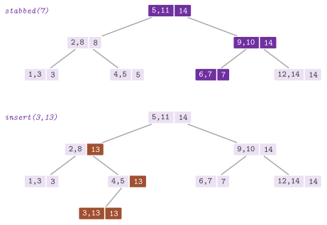
order, \(g( a , b ) = b\) and \(\oplus = \max\) (the augmentation MaxEnd). Its
identity is no interval, an empty std::optional, which is below any end; a
sentinel such as the least value of the type would not do for the floating
types, whose intervals may end at \(-\infty\) (cf. exercise 11). The
augmentation of a node is thus the largest right end of its subtree (Figure
16.4). A stabbing query looks for the intervals
that contain a point \(x\).
Lemma 16.9. An interval of the tree \(T\) contains \(x\) if and only if
Proof. \([ a , b ]\) contains \(x\) if and only if \(a \le x\) and \(b \ge x\); hence one of the intervals with \(a \le x\) contains \(x\) if and only if the largest of their right ends is at least \(x\). \(\square\)
The intervals with \(a \le x\) form a prefix of the order of the keys, the
keys up to \(( x , +\infty )\). This prefix is the union of the nodes at
which the search for \(( x , +\infty )\) goes right and of their left
subtrees, and stabbed() reads the maximum of (16.9) along that path in
\(O( \log n )\) time (Algorithm 16.6).
Algorithm 16.6. The stabbing query of an interval tree on an augmented map (Sun and Blelloch 2019); \(m\) is the largest right end of the intervals with \(a \le x\) met so far.
To report the intervals, stab() visits the tree in symmetric order, and
it reports them by increasing \(( a , b )\). However, it enters a subtree
only if its augmented value is at least \(x\), and it does not go right of a
node with \(a > x\) (Algorithm 16.7); count()
counts the calls that stab() makes.
Algorithm 16.7. The report of the intervals that contain \(x\) (Sun and Blelloch 2019).
Lemma 16.10. stab( x , f ) calls \(f\) once
per copy of each interval that contains \(x\), by increasing \(( a , b )\), in
\(O( \min( n , ( k + 1 ) \log n ) )\) time plus the calls, \(k\) being the number
of distinct intervals reported.
Proof. A subtree whose augmented value is below \(x\) holds no interval with \(b \ge x\), and the nodes right of a node with \(a > x\) have \(a > x\) too; hence the visit skips no interval that contains \(x\), and line 5 reports exactly those. As for the time, a node visited is either on the search path of \(( x , +\infty )\), of length \(O( \log n )\), or in a left subtree hanging from that path. In the second case all the keys of the subtree have \(a \le x\), and the node, since it is entered, has in its subtree an interval with \(b \ge x\), which is reported. Each node visited is thus on the search path or on the path from the root to a reported interval: there are at most \(( k + 1 ) \, O( \log n )\) of them, and at most \(n\). \(\square\)
This bound is worse than the \(O( \log n + k )\) of the interval tree of Edelsbrunner 1980 and of the priority search tree of McCreight 1985, which are structures built for this query. On the other hand, the augmented map is an ordered map with its own updates in \(O( \log n )\), and the same code serves the range tree below. Cormen et al. 2009, §14.3 build the interval tree on a red-black tree in the same way, and use it to find one interval that contains \(x\) in \(O( \log n )\) time.
16.4.2 The range tree¶
RangeTree< T > keeps a multiset of points \(( x , y )\) of a type T that is
totally ordered and has std::numeric_limits (the points are the type Point
of the class, a std::pair, not the Point of ConvexHull.h). The keys are
in lexicographic order, and \(g( x , y )\) is the sequence \(( y )\), with \(c\)
copies of \(y\) for a point of multiplicity \(c\) (the augmentation Ordinates);
\(\oplus\) is the merge of two sorted sequences, whose identity is the empty
one. The augmentation of a node is then the sorted sequence of the ordinates
of its subtree, as in the range tree of Bentley
1980, while the map orders the points by
\(x\) (Figure 16.5).
Lemma 16.11. A RangeTree of \(n\) points
takes \(O( n \log n )\) space, \(\Theta( n \log n )\) when the points are
distinct, and its construction \(O( n \log n )\) time.
Proof. The ordinate of a point is in the sequence of each of its ancestors and of its own node, which are \(O( \log n )\) in a tree balanced by weight. Summing over the points gives \(O( n \log n )\). For distinct points the sum is the sum of the depths plus \(n\), and in any binary tree at most \(2^d\) nodes have depth \(d\), so that the sum is at least \(\sum_{i=1}^{n} \lfloor \log_2 i \rfloor = \Omega( n \log n )\) (with repetitions it may be smaller, e.g., \(n\) for \(n\) copies of one point). The construction by joins of balanced halves merges each sequence once per level of the recursion, i.e., \(O( n )\) work per level on \(O( \log n )\) levels. \(\square\)
The points of \([ x_1 , x_2 ] \times [ y_1 , y_2 ]\) are those whose keys lie
between \(( x_1 , -\infty )\) and \(( x_2 , +\infty )\) and whose ordinate lies
in \([ y_1 , y_2 ]\). count() returns 0 on an empty rectangle (\(x_2 < x_1\) or \(y_2 < y_1\));
otherwise it covers the range of the keys by the
\(O( \log n )\) pieces of augVisit(), and in each piece it counts the
ordinates in \([ y_1 , y_2 ]\) by two binary searches on the sorted sequence
(Algorithm 16.8). For the infinities it uses
-infinity() and infinity() in the types that have them, so that a
point with \(y = \pm \infty\) at the abscissa \(x_1\) or \(x_2\) is counted too,
and lowest() and max() in the others.
Algorithm 16.8. The count of the points in a rectangle, on the range tree of Bentley 1980 built as an augmented map.
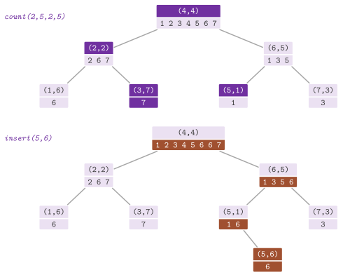
Lemma 16.12. count() returns the number
of points of the rectangle, with their copies, in \(O( \log^2 n + c )\) time,
\(c\) being the copies of the single points among its pieces, i.e., in
\(O( \log^2 n )\) time for points without repetitions; an insertion or a
removal takes \(O( n )\) time.
Proof. By construction, the pieces are disjoint and cover the keys of the range. In the sorted sequence \(Y\) of a piece, the ordinates in \([ y_1 , y_2 ]\) are those between the first one not below \(y_1\) and the first one above \(y_2\), which two binary searches find in \(O( \log n )\) time. A whole subtree passes its sequence by reference, whereas a single node builds a sequence of its \(c\) copies, at a cost \(O( c )\) (i.e., \(O( 1 )\) for points without repetitions). An insertion or a removal changes the sequences of all the ancestors of its point, and the root's has \(n\) ordinates. \(\square\)
The fractional cascading of Lueker 1978 and Willard 1985 (in general, Chazelle and Guibas 1986) would remove one factor \(\log n\) from Lemma 16.12, by pointers from each sequence into those of the two children; yet, every merge would have to rebuild them. The dynamic range tree of Sun and Blelloch 2019 keeps the updates in \(O( \log^2 n )\) by sharing the inner trees between persistent versions, which the maps of ADS, being destructive, do not. Table 16.3 summarizes the two structures.
Table 16.3. The two augmented maps of
ADS/geometry; \(k\) is the number of distinct intervals reported.
| Structure | Augmentation | Query | Update | Space |
|---|---|---|---|---|
IntervalTree |
the largest right end | stabbed() \(O( \log n )\), stab() \(O( \min( n , ( k + 1 ) \log n ) )\) |
\(O( \log n )\) | \(\Theta( n )\) |
RangeTree |
the sorted ordinates | count() \(O( \log^2 n )\) |
\(O( n )\); \(O( n \log n )\) to build | \(\Theta( n \log n )\) |
16.5 Discussion and references¶
The convex hull and the closest pair are the problems with which the textbooks of computational geometry usually begin; Preparata and Shamos 1985 treat both, with the lower bounds of Theorem 16.1 and of (16.6). The hull by checking every segment and the scan of Graham are those of Montresor 2025, §16.1, where the scan is an example of backtracking. As for the sources, the scan is from Graham 1972, the monotone chain from Andrew 1979, and the filter of the extreme points from Akl and Toussaint 1978, with the expected analysis of Devroye and Toussaint 1981. There is no algorithm whose time depends on the size \(h\) of the output (say, the gift wrapping in \(O( n h )\)) in the library, and no hull in three or more dimensions.
Montresor 2025 does not treat the closest pair, but its divide and conquer of chapter 12 is the scheme used here. The algorithm in \(O( n \log n )\) is from Shamos and Hoey 1975, the sweep from Hinrichs, Nievergelt and Schorn 1988, and the randomized algorithms in \(O( n )\) expected time from Rabin 1976, Khuller and Matias 1995 and Golin et al. 1995. All the algorithms of the chapter work on integer coordinates bounded by \(10^9\), which makes them exact by Lemma 16.1; points with floating coordinates would need the adaptive predicates of the robust geometric libraries, which ADS does not have.
The range tree is from Bentley 1979
and Bentley 1980, the interval tree
from Edelsbrunner 1980, and the
priority search tree from McCreight
1985. Writing both structures as
augmented maps follows Sun and Blelloch 2019,
who also give the segment and the rectangle queries; the parallel
construction of multiInsert() is from Sun, Ferizovic and Blelloch
2018. The comparison of the hulls and of
the closest pairs with those of other libraries (e.g., Boost.Geometry and
CGAL), and of the two maps with structures built for their queries, belongs
to the campaign of benchmarks of appendix B, and
it is not reported here.
16.6 Exercises¶
Each exercise names the test of the library that solves it (run it with
ctest -R <name>).
- Decide whether two points lie on the same side of the line through two
others, the points on the line counting on both sides, also when the
two points of the line coincide and with coordinates of \(10^9\)
(Montresor 2025, §16.1). Test:
ch16.sec16.1.same-side. - Give an increasing function of the angle of a vector that uses no
trigonometric function, and check that its values stay in \([ 0 , 4 )\)
for the extreme components of a
long(Montresor 2025, exercise 16.1). Test:ch16.ex16.1. - Compute the convex hull by the scan of Graham and check it against the
hull by checking every segment, on random points with many collinear
ones, on points that are all collinear and on points on the sides of a
triangle. Test:
ch16.sec16.1.hull. - Check that a polygon is the convex hull of a set of points (convex,
counterclockwise, made of points of the set, containing all of them),
and refuse the coordinates beyond \(10^9\) in absolute value. Test:
contract_geometry.hull. - Reduce the sort of \(n\) numbers to the convex hull of \(n\) points in
\(O( n )\) time, and conclude Theorem 16.1.
Test:
ch18.sec18.5.hull-sort. - Compute the hull with the filter of the octagon, a radix sort and the
monotone chain, and check that it equals the output of the scan of
Graham on points uniform in a square and in a disk, near a circle and on
small grids with many ties. Test:
engineered_numeric.convex-hull. - Find the closest pair of \(n\) points in \(O( n \log n )\) time by divide
and conquer, with repeated points, collinear points and coordinates of
\(10^9\). Tests:
lib_search.closest-pair,contract_geometry.closest-pair. - Find the closest pair by a sweep on the points sorted by radix, falling
back on the randomized grid on the inputs on which the sweep takes too
long, such as points on a column or on a row with growing gaps. Test:
engineered_numeric.closest-pair-sweep. - Keep a multiset of intervals under insertions and removals, answer in
\(O( \log n )\) whether an interval contains a point, and report the
intervals that contain it by increasing left end. Test:
join_trees.interval-tree. - Keep a multiset of points and count those in a rectangle in
\(O( \log^2 n )\) time. Test:
join_trees.range-tree. - Make both structures correct when the coordinates and the ends are
the infinities of a floating type. Test:
join_trees.infinite-bounds.