13. Algorithm design¶
[Source: include/ADS/algorithm/MasterTheorem.h, AkraBazzi.h,
BinaryCounter.h, Hanoi.h, Paradigms.h, MaximumSegments.h,
Subsequences.h, SequenceQueries.h, MonteCarlo.h;
include/ADS/optimization/Knapsack.h, KnapsackVariants.h,
CoinChange.h, WeightedIntervals.h, HouseProblems.h,
StockTrading.h, SequenceProblems.h, CoinGame.h,
OptimalSearchTree.h, LinearPartition.h, GridPaths.h,
FractionalKnapsack.h, Intervals.h, IntervalCover.h,
ShortestJobFirst.h]
We are concerned in this chapter with the techniques by which an algorithm
is designed, and with the tools by which its cost is found. In ADS/algorithm, the headers collect the tools (the solution of the recurrences, the
amortized analysis, the elimination of the recursion), the general schemes
of the techniques, and a few families of algorithms on sequences that
illustrate them; those of ADS/optimization solve problems of optimization
by the two techniques that most of the course is about, i.e., the dynamic
programming and the greedy algorithms. We follow the order in which the
techniques build on each other, which is (more or less) that of a course. Sections 13.1
and 13.2 give the costs of the recursive
algorithms and of the sequences of operations, §13.3
turns a recursion into an iteration, and §13.4
writes each technique once as a scheme. Sections
13.5 and 13.6 solve
problems on sequences by scans, sorts and sliding windows, where the gain
over the enumeration comes from a property of the optimal solutions;
sections 13.7 to 13.10
are devoted to the dynamic programming, grouped by the shape of the
subproblems, §13.11 to the greedy algorithms
and to the exchange arguments that prove them optimal, and
§13.12 to the algorithms of Monte Carlo.
Throughout the chapter we write \(n\) for the size of the input (the number of items,
objects, intervals or keys), and we take the logarithms binary unless their
base is written. In the sets of §1.9, the
headers of this chapter are all base.
13.1 Orders of growth and recurrences¶
As usual, the cost of an algorithm is a function \(T( n )\) of the size \(n\) of its input, and it is compared with others by its order of growth: \(f( n ) = O( g( n ) )\) if \(f( n ) \le c \, g( n )\) for some \(c > 0\) and all the \(n\) large enough, \(f( n ) = \Omega( g( n ) )\) if \(g( n ) = O( f( n ) )\), and \(f( n ) = \Theta( g( n ) )\) if both hold (Montresor 2025, chapter 2). All the orders that the recurrences of this section produce are all of the form
which the structure Growth of MasterTheorem.h stores as its four
exponents \(c\), \(p\), \(q\) and \(r\), together with a flag upper for a bound
that is only an upper one (\(O\) instead of \(\Theta\)). Two orders (13.1)
compare as their functions do for \(n\) large, i.e., lexicographically on
\(( c , p , q , r )\), since each factor dominates any power of the factors
after it; this is the comparison operator<=> of Growth (with the operator== that
follows from it), which ignores upper, while at( n ) evaluates the function
(13.1) at \(n\), with natural logarithms (the base changes the value, not
the order); the comparison gives the hierarchy \(1 \prec \log n \prec n \prec n \log n
\prec n^2 \prec n^3 \prec 2^n\). Note that \(2^{\log_2 n} = n\) is a
polynomial, and that the orders that lie between two families, such as
\(n^{\log n}\) (which grows faster than every polynomial and slower than
every \(c^n\) with \(c > 1\)), have no place in (13.1).
An algorithm of divide et impera that splits an instance of size \(n\) into \(a\) instances of size \(n / b\), and spends \(g( n ) = \Theta( n^\beta \log^k n )\) to divide it and to combine the solutions, costs
Theorem 13.1 (the master theorem). Let \(a \ge 1\), \(b > 1\) and \(\alpha = \log_b a\). Then the solution of (13.2) is \(\Theta( n^\alpha )\) if \(\beta < \alpha\), and \(\Theta( n^\beta \log^k n )\) if \(\beta > \alpha\); if \(\beta = \alpha\), it is \(\Theta( n^\alpha \log^{k+1} n )\) for \(k > -1\), \(\Theta( n^\alpha \log \log n )\) for \(k = -1\), and \(\Theta( n^\alpha )\) for \(k < -1\).
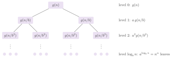
Proof. The tree of the recursion (Figure 13.1) has \(\log_b n\) levels, and its level \(j\) has \(a^j\) nodes of size \(n / b^j\), which cost in all
If \(\beta < \alpha\), then \(a / b^\beta > 1\) and the terms (13.3) grow geometrically towards the leaves, whose \(a^{\log_b n} = n^\alpha\) nodes dominate the sum; if \(\beta > \alpha\), they decrease geometrically and the root dominates. If \(\beta = \alpha\), the level \(j\) costs \(\Theta( n^\alpha \log^k ( n / b^j ) )\), and the sum over the levels is, up to a constant, that of \(i^k\) for \(i\) from 1 to \(\log_b n\), i.e., \(\Theta( \log^{k+1} n )\) for \(k > -1\), the harmonic sum \(\Theta( \log \log n )\) for \(k = -1\), and a convergent series for \(k < -1\). That the floors and the ceilings of the sizes change no order is the result of Leighton 1996 quoted below for (13.4), of which (13.2) is the case of one term, \(a_1 = a\) and \(b_1 = 1 / b\). \(\square\)
For \(k = 0\) this is Theorem 2.2 of Montresor
2025, and the general case is its
Theorem 2.4. In the library, master( a , b , beta , k ) decides among the
five cases (Algorithm 13.1), and returns the
order as a Growth. Since \(\log_b a\) is computed in floating point, a
value of it within \(10^{-12}\) of an integer is taken as that integer, and
\(\beta\) is compared with \(\alpha\) with the same tolerance; without the
rounding, \(\log_{10} 1000\) comes out as \(2.9999999999999996\), and the
recurrence \(T( n ) = 1000 \, T( n / 10 ) + n^3\) would be moved from the
third case to the second one.
Algorithm 13.1. The master theorem (Montresor 2025, §2.9).
When the parts have "different" sizes, as in \(T( n ) = T( n / 5 ) + T( 7 n / 10 ) + n\) of the selection in linear time, the master theorem does not apply. For \(T( n ) = \sum_{i=1}^k a_i T( b_i n ) + g( n )\), with \(a_i > 0\) and \(0 < b_i < 1\), the theorem of Akra and Bazzi 1998 replaces \(\alpha\) by the real \(p\) such that
and Leighton 1996 showed that the floors and the ceilings of the sizes, and perturbations of them of \(O( n / \log^2 n )\), do not change the order.
Theorem 13.2 (Akra and Bazzi). The equation \(f( p ) = \sum_i a_i b_i^p = 1\) has a unique real root \(p\), and for \(g( n ) = \Theta( n^\beta \log^k n )\) the order (13.4) is that of Theorem 13.1 with \(p\) in place of \(\alpha\).
Proof. Each term \(a_i b_i^p\) is strictly decreasing in \(p\), since \(0 < b_i < 1\), and it goes from \(+\infty\) to 0; hence so does \(f\), and its root is unique. With \(g( u ) = u^\beta \log^k u\) the integrand of (13.4) is \(u^{\beta - p - 1} \log^k u\) (for \(k < 0\), \(g\) is defined only for \(u > 1\), and we start the integral at \(u = 2\), which changes it by a constant), whose integral up to \(n\) is \(\Theta( 1 )\) for \(\beta < p\) and \(\Theta( n^{\beta - p} \log^k n )\) for \(\beta > p\), while for \(\beta = p\) it is \(\int_2^n \log^k u \, du / u\), i.e., \(\Theta( \log^{k+1} n )\), \(\Theta( \log \log n )\) or \(\Theta( 1 )\) as \(k\) is larger than, equal to or smaller than \(-1\). \(\square\)
akraBazziExponent() finds the root by bisection
(Algorithm 13.2). It first brackets it by
doubling: starting from \(\mathit{lo} = -1\) and \(\mathit{hi} = 1\), it
doubles \(\mathit{lo}\) (towards \(-\infty\)) while \(f( \mathit{lo} ) < 1\), and
\(\mathit{hi}\) while \(f( \mathit{hi} ) > 1\), which ends since \(f\) goes from
\(+\infty\) to 0. Then it halves the bracket 200 times, which leaves an
interval far below the resolution of a double around the root; its
postcondition checks that \(\lvert f( p ) - 1 \rvert < 10^{-9}\).
akraBazzi() then applies the five cases with \(p\), with a tolerance of
\(10^{-9}\) on the comparison of \(\beta\) with \(p\). In the example of the
selection, \(( 1 / 5 )^p + ( 7 / 10 )^p = 1\) gives \(p \approx 0.8398 < 1 =
\beta\), and the selection is linear.
Algorithm 13.2. The exponent of Akra and Bazzi by bisection, and the order of the recurrence.
Recurrences that decrease the size by a constant, \(T( n ) = \sum_{i=1}^h a_i T( n - i ) + \Theta( n^\beta )\), unfold instead into a tree of depth \(\Theta( n )\).
Theorem 13.3. Let \(a = \sum_{i=1}^h a_i\), with the \(a_i\) integers not negative, and \(\beta \ge 0\). If \(a = 1\), then \(T( n ) = \Theta( n^{\beta + 1} )\); if \(a \ge 2\), then \(T( n ) = O( a^n n^\beta )\).
Proof. With \(a = 1\) the recurrence is \(T( n ) = T( n - i ) + \Theta( n^\beta )\) for one \(i\), and it unfolds into a path of \(n / i\) nodes whose costs sum to \(\Theta( n^{\beta + 1} )\). With \(a \ge 2\), the tree has at most \(a^j\) nodes at the depth \(j \le n\), each of cost \(O( n^\beta )\), and the sum is \(O( a^n n^\beta )\). \(\square\)
Note that the second bound is an upper one only, since the branches of different
depths make the tree smaller than a full one: the recurrence of Fibonacci,
with \(a = 2\), is \(\Theta( \phi^n )\), \(\phi = ( 1 + \sqrt 5 ) / 2\); hence
linear( a , beta ) (Algorithm 13.3) returns
it with the flag upper. Also, the theorem (Theorem 2.5 of Montresor
2025) has integer \(a_i\); for real
\(a_i\) with \(1 < a < 2\), e.g., \(T( n ) = 1.5 \, T( n - 1 ) + 1 = \Theta(
1.5^n )\), the recurrence is exponential as well, and linear() gives the
same upper bound. Table 13.1 collects the
recurrences of the algorithms of the library that the three functions
solve.
Algorithm 13.3. The recurrences that decrease the size by a constant.
Table 13.1. Some recurrences and the
orders that master(), akraBazzi() and linear() return for them.
| Algorithm | Recurrence | Call | Order |
|---|---|---|---|
| binary search | \(T( n / 2 ) + 1\) | master(1,2,0) |
\(\Theta( \log n )\) |
| mergesort | \(2 T( n / 2 ) + n\) | master(2,2,1) |
\(\Theta( n \log n )\) |
| Strassen | \(7 T( n / 2 ) + n^2\) | master(7,2,2) |
\(\Theta( n^{\log_2 7} )\) |
| (an example) | \(2 T( n / 2 ) + n / \log n\) | master(2,2,1,-1) |
\(\Theta( n \log \log n )\) |
| selection in linear time | \(T( n / 5 ) + T( 7 n / 10 ) + n\) | akraBazzi({{1,0.2},{1,0.7}},1) |
\(\Theta( n )\) |
| towers of Hanoi | \(2 T( n - 1 ) + 1\) | linear(2,0) |
\(O( 2^n )\) |
| insertion sort | \(T( n - 1 ) + n\) | linear(1,1) |
\(\Theta( n^2 )\) |
In the library the three solvers of the recurrences are declared as
follows, Growth being the structure of (13.1):
// declarations of <ADS/algorithm/MasterTheorem.h> <ADS/algorithm/AkraBazzi.h>
Growth master( double a , double b , double beta , double k = 0 );
Growth linear( double a , double beta );
double
akraBazziExponent( const std::vector< std::pair< double , double > > & ab );
Growth akraBazzi( const std::vector< std::pair< double , double > > & ab ,
                  double beta , double k = 0 );
13.2 Amortized analysis¶
We call amortized cost of an operation its share of the total cost of any
sequence of operations, which may be much less than its cost in the worst
case (Tarjan 1985). A binary counter
of \(k\) bits, in BinaryCounter.h, is the example of Montresor 2025,
§4.2.1: the counter is a vector
\(A[ 0 .. k - 1 ]\) of bits, \(A[ 0 ]\) the least significant, and add( A )
increments it modulo \(2^k\) by clearing the ones at the bottom and setting
the first zero (Algorithm 13.4 and
Figure 13.2). It returns the number of bits
that it has changed, i.e., its actual cost, which is \(k\) when the counter
is full of ones (all of them are cleared, and none is set).

Algorithm 13.4. The increment of a binary counter (Montresor 2025, §4.2.1).
Lemma 13.1. Starting from a counter of
zeros, \(n\) increments change fewer than \(2 n\) bits; hence the amortized
cost of add() is \(O( 1 )\).
Proof. By aggregation: the bit \(A[ i ]\) changes once every \(2^i\) increments, i.e., \(\lfloor n / 2^i \rfloor\) times, and
By a potential: let \(\Phi\) be the number of ones of the counter, which starts at 0 and is never negative. An increment that clears \(d\) bits and sets one costs \(d + 1\) and changes \(\Phi\) by \(1 - d\), and therefore its amortized cost \(d + 1 + \Delta \Phi\) is 2; the increment that wraps around clears \(k\) bits and sets none, and its amortized cost is \(k - k = 0\). Hence the total cost is at most \(2 n\) minus the final potential. \(\square\)
We remark that the method of the potential is the one that the other structures of the
library typically use, e.g., the splay tree (§8.8) and the Fibonacci heap (§9.7), since it charges
each operation by the state that it leaves instead of by a count over the
sequence. Also, the contracts of add() check, as an audit, that the items of
\(A\) are bits, and that at most \(k\) of them change.
The counter is a vector of int, each 0 or 1, and the increment is
declared as
13.3 Recursion and its elimination¶
A recursive procedure runs on the stack of the calls, and it can be made
iterative by keeping that stack by hand (Montresor 2025,
§4.4). In Hanoi.h, the towers of Hanoi
are the example: \(n\) disks of different sizes lie on the peg
source, and they must be moved to the peg dest, one at a time and never
on a smaller disk, with the peg middle as a spare. Its recursive
procedure (hanoi_recursive(), Algorithm 13.5) moves the \(n - 1\)
smaller disks on middle (the call (1)), the largest one on dest, and
the \(n - 1\) disks on dest (the call (2)). Each of the three functions of
the header hands each move to a function f( from , to ) given by the
caller, and a test can thus check the sequence of the moves.
Algorithm 13.5. The towers of Hanoi by recursion (Montresor 2025, §4.4).
Lemma 13.2. The recursive procedure makes \(T( n ) = 2 T( n - 1 ) + 1 = 2^n - 1\) moves, and no procedure makes fewer.
Proof. The recurrence, with \(T( 1 ) = 1\), gives \(2^n - 1\) by induction.
For the lower bound, let \(M( n )\) be the fewest moves of \(n\) disks from a
peg to another; we show \(M( n ) \ge 2^n - 1\) by induction, \(M( 1 ) = 1\)
being clear. The largest disk must move at least once, and it can move
only when the other \(n - 1\) disks are all on the peg that is neither its
origin nor its destination, since none of them may lie under it or on the
peg that receives it. Before its first move, the \(n - 1\) smaller disks have
therefore been moved from the peg source to one other peg, which takes at
least \(M( n - 1 )\) moves (the largest disk, which stays at the bottom, does
not constrain them); after its last move, which ends on dest, they are
moved from one peg onto dest, at least \(M( n - 1 )\) moves more. Hence
\(M( n ) \ge 2 M( n - 1 ) + 1 \ge 2 ( 2^{n-1} - 1 ) + 1 = 2^n - 1\). \(\square\)
A first iterative procedure (hanoi_iterative(),
Algorithm 13.6) pushes the parameters of each
call (1) on a stack, and changes the parameters to those of the call;
when it pops a frame, it resumes the call left open, moves its disk, and
simulates the call (2) by changing the parameters once more instead of
pushing them. This is the elimination of a tail call: since the call (2)
is the last action of the procedure, nothing of its caller needs to be
saved. The second procedure (hanoi_iterative_labels(),
Algorithm 13.7) applies instead the systematic
rules, which apply to any recursion: a call pushes the parameters together
with the label from which the caller resumes (AFTER1 after the call (1),
END after the call (2)), a return pops them, and the procedure becomes a
loop over the labels START, AFTER1, END and STOP.
Table 13.2 follows the first one on three
disks.
Algorithm 13.6. The towers of Hanoi with the calls (1) on a stack and the call (2) eliminated.
Algorithm 13.7. The towers of Hanoi by the systematic rules, with the label of the point of return on the stack.
Table 13.2. hanoi_iterative() on \(n = 3\)
disks from the peg A to the peg C: the stack after each step (its top on
the right), a frame being \(( n , \mathit{src} , \mathit{dest} ,
\mathit{mid} )\), and the moves.
| Step | Stack | Move |
|---|---|---|
| push, push | \(( 3 , A , C , B ) \; ( 2 , A , B , C )\) | |
| \(n = 1\) | \(( 3 , A , C , B ) \; ( 2 , A , B , C )\) | A \(\to\) C |
| pop | \(( 3 , A , C , B )\) | A \(\to\) B |
| \(n = 1\) | \(( 3 , A , C , B )\) | C \(\to\) B |
| pop | A \(\to\) C | |
| push | \(( 2 , B , C , A )\) | |
| \(n = 1\) | \(( 2 , B , C , A )\) | B \(\to\) A |
| pop | B \(\to\) C | |
| \(n = 1\), stack empty | A \(\to\) C |
Both stacks are ArrayStacks (§3.2), of capacity
\(n\) and \(2 n\). Indeed, each holds at most one frame per level of the recursion
that is open, i.e., fewer than \(n\) frames, since in the second procedure
the frame with the label END replaces the one with AFTER1 that was just
popped; the time of all three procedures is \(\Theta( 2^n )\), i.e., a
constant per move.
The three procedures have the same parameters, the number of the disks, the three pegs and the function that receives each move:
// declarations of <ADS/algorithm/Hanoi.h>
template< class F >
void hanoi_recursive( int n , int source , int dest , int middle , F && f );
template< class F >
void hanoi_iterative( int n , int source , int dest , int middle , F && f );
template< class F >
void hanoi_iterative_labels( int n , int source , int dest , int middle ,
                             F && f );
13.4 The general schemes¶
In Paradigms.h, the functions write the techniques of chapters 12 to 16 of
Montresor 2025 once, in terms of the
parts that make a technique concrete, each part being a function given by
the caller. A problem is a quintuple \(\langle I , S , R , O , Q \rangle\):
the instances \(I\), the solutions \(S\), the relation \(R \subseteq I \times S\)
between them, the answers \(O\) and the function \(Q\) that gives the answer
of an instance. In a problem of search, the answer of \(i\) is a solution \(s\)
with \(\langle i , s \rangle \in R\), or none (written \(\bot\)); in a problem
of decision it is whether such an \(s\) exists, which may (but need not) be
found by the search; in a problem of optimization it is a solution that is
best for a measure \(m\) with values in an ordered set, or none. A search
space \(Z\) of an instance is a set of objects with a function of
admissibility \(a\) and one of answer \(o\), such that \(a( z )\) holds if and
only if \(o( z )\) is a solution; for a problem of optimization, \(Z\) must
also contain an optimal solution.
In the enumerative method one lists \(Z\) in a total order, given by its first
object and the functions next() and last(). enumerateSearch() returns
the answer of the first admissible object, or nothing
(Algorithm 13.8); enumerateOptimize()
examines all of \(Z\) and returns the answer of the first admissible object
with no admissible one strictly better for the relation better() on the
measures (Algorithm 13.9). Both cost \(\lvert Z
\rvert\) evaluations of \(a\) in the worst case, which is usually
exponential in \(n\) (cf. Theorem 13.3).
Algorithm 13.8. The enumerative search.
Algorithm 13.9. The enumerative optimization.
Backtracking (backtrack(), Algorithm 13.10)
lists \(Z\) as the leaves of a tree of partial solutions: the root is the
empty one, and a node at the level \(j\) has a child for each way of adding
the component \(j + 1\). A node that prune() rejects is not visited, and its
subtree with it; hence, backtracking is (possibly much) faster than the
enumeration when the rejections come "early"; each leaf goes to visit(),
which returns true to stop the visit. Chapter 19 is devoted to its uses.
A greedy algorithm (greedy(), Algorithm 13.11)
builds a solution by \(k\) stages, appending at each one the best of the
values that candidates() declares admissible after the partial solution
built so far, and it never goes back; a stage with no candidate is skipped.
It is correct only for the (rather few) problems where an exchange argument shows that
some optimum agrees with each choice (§13.11).
Divide et impera (divideEtImpera(),
Algorithm 13.12) solves an instance directly
if it is "small", and otherwise divides it into instances of the same
problem, solves them recursively and combines their solutions; its cost is
a recurrence such as (13.2) (cf. Theorem 13.1). Finally, when the measure is only partially
ordered, the answers of a problem of optimization are the maximal
solutions, those with no solution strictly better, which maximal() finds
by comparing all the pairs (Algorithm 13.13),
i.e., with \(O( n^2 )\) calls of better() on \(n\) elements.
Algorithm 13.10. The scheme of backtracking (Montresor 2025, chapter 16).
Algorithm 13.11. The greedy scheme (Montresor 2025, chapter 14).
Algorithm 13.12. The scheme of divide et impera (Montresor 2025, chapter 12).
Algorithm 13.13. The maximal elements of a partial order.
We remark that the schemes are generic in the strict sense: they know nothing of the
problem, and the cost of an algorithm written through them is that of the
parts given by the caller times the number of times that the scheme calls
them. Furthermore, the test beyond.paradigms instantiates each of them: the linear
search and the sort by the enumeration of the permutations, the 0-1
knapsack by the enumeration of the subsets (checked against knapsack() of
§13.7), the \(n\) queens by backtracking, the
minimum and the maximum by divide et impera, the change by the greedy
scheme, and the maximal words of a list for three partial orders.
Each part of a scheme is a callable given by the caller, and the schemes are declared as follows:
// declarations of <ADS/algorithm/Paradigms.h>
template< class Z , class Next , class Last , class A , class O >
auto enumerateSearch( Z z , Next && next , Last && last , A && a , O && o )
  -> std::optional< decltype( o( z ) ) >;
template< class Z , class Next , class Last , class A , class O , class M ,
          class B >
auto enumerateOptimize( Z z , Next && next , Last && last , A && a , O && o ,
                        M && m , B && better )
  -> std::optional< decltype( o( z ) ) >;
template< class N , class C , class P , class L , class V >
bool backtrack( const N & node , C && children , P && prune , L && leaf ,
                V && visit );
template< class X , class Cand , class Best >
std::vector< X > greedy( int k , Cand && candidates , Best && best );
template< class X , class S , class D , class V , class C >
auto divideEtImpera( const X & x , S && small , D && direct , V && divide ,
                     C && combine ) -> decltype( direct( x ) );
template< class T , class B >
std::vector< T > maximal( const std::vector< T > & X , B && better );
13.5 Segments of largest sum¶
Given an array \(D[ 0 .. n - 1 ]\) of numbers, a segment \(D[ b .. s ]\) is a run of consecutive items, and we look for a nonempty segment of largest sum (Ferragina 2023, chapter 2; Bentley 1984). Its items may be, e.g., the daily gains of a stock (the differences of its quotations), and then the segment is the best period in which to hold it; or the scores of the nucleotides of a DNA sequence, and then the segment is the region richest in some of them. With the prefix sums
the segment \(D[ b .. s ]\) sums to \(P[ s + 1 ] - P[ b ]\). A Segment of
MaximumSegments.h holds the sum of \(D[ \mathit{first} .. \mathit{first} +
\mathit{length} - 1 ]\), with length 0 for none; the sums of the segments
and of the prefixes must fit in the type of the items, which is not
checked.
In Ferragina 2023, chapter
2, four algorithms are given, which differ in what they reuse.
maxSumSegmentCubic() tries all the pairs \(( b , s )\) and recomputes each
sum, in \(\Theta( n^3 )\) time; maxSumSegmentQuadratic() extends the sum of
\(D[ b .. s - 1 ]\) to that of \(D[ b .. s ]\), in \(\Theta( n^2 )\) time. The
linear scan (maxSumSegment(), Algorithm 13.14),
which is usually credited to Kadane, rests on two properties of the optimal
segments.
Algorithm 13.14. The segment of largest sum by one scan.
Lemma 13.3. (i) An optimal segment has no proper prefix of negative sum. (ii) If the prefixes of \(D[ b .. s ]\) have sums not negative, then for each \(b' \in ( b , s ]\) the segment \(D[ b .. s ]\) has a sum at least as large as \(D[ b' .. s ]\). Hence the scan, which restarts after the place where the running sum becomes negative, finds an optimal segment in \(O( n )\) time.
Proof. (i) Removing a proper prefix of negative sum would leave a nonempty segment of larger sum. (ii) \(D[ b .. s ]\) is \(D[ b' .. s ]\) extended by the prefix \(D[ b .. b' - 1 ]\), whose sum is not negative. Let \(D[ b^* .. s^* ]\) be optimal, and let \(b\) be the current start of the scan at the step \(s^*\), before the test of the restart. If \(b \le b^*\), the scan did not restart between \(b\) and \(s^*\), the prefixes of \(D[ b .. s^* - 1 ]\) have sums not negative, and by (ii) the sum compared at the step \(s^*\) is at least that of the optimum. If \(b > b^*\), consider the first restart at a step \(r \ge b^*\), which happens before \(s^*\): the start \(b'\) current at that time is at most \(b^*\), and the prefixes of \(D[ b' .. r - 1 ]\) have sums not negative, while \(D[ b' .. r ]\) has a negative one. Then \(D[ b^* .. r ]\), which is \(D[ b' .. r ]\) without the prefix \(D[ b' .. b^* - 1 ]\) of sum not negative, has a negative sum, and it is a proper prefix of the optimum, against (i). \(\square\)
Table 13.3 follows the scan on an example.
Note that the scan reads the array once, from left to right; in a memory of blocks of
\(B\) items it makes \(\lceil n / B \rceil\) transfers, whatever \(B\), and the
algorithm is therefore cache oblivious. Since the best segment is initialized
with \(D[ 0 ]\), a segment is never empty, and an array of negative numbers
gives its largest item. maxSubarraySum() of Subsequences.h is the same
scan for the value only, \(t \gets \max\{ t + a , 0 \}\), with the empty
subvector of sum 0 allowed (Montresor 2025, exercises 12.2 and
13.12); the two agree whenever the
best sum is not negative, which the contracts of maxSumSegment() check as
an audit.
Table 13.3. maxSumSegment() on
\(D = ( 2 , -3 , 4 , -1 , -2 , 1 , 5 , -3 )\): the running sum \(x\) and the
current start \(b\) after each step, and the best segment as (sum, first,
length).
| \(s\) | \(D[ s ]\) | \(x\) | \(b\) | best |
|---|---|---|---|---|
| 0 | 2 | 2 | 0 | (2, 0, 1) |
| 1 | \(-3\) | 0 (restart) | 2 | (2, 0, 1) |
| 2 | 4 | 4 | 2 | (4, 2, 1) |
| 3 | \(-1\) | 3 | 2 | (4, 2, 1) |
| 4 | \(-2\) | 1 | 2 | (4, 2, 1) |
| 5 | 1 | 2 | 2 | (4, 2, 1) |
| 6 | 5 | 7 | 2 | (7, 2, 5) |
| 7 | \(-3\) | 4 | 2 | (7, 2, 5) |
Another linear algorithm of Ferragina 2023, chapter 2 reads the problem on the prefix sums: the best segment that ends in \(s\) sums to
and maxSumSegmentPrefix() carries the minimum along the scan
(Algorithm 13.15). It is the form (13.7) that
generalizes to the variants below.
Algorithm 13.15. The segment of largest sum by the least prefix sum.
Segments of bounded length. With the length of the segment bounded to
\([ L , U ]\), \(1 \le L \le U\), the minimum of (13.7) is taken over the
window of the starts \(x \in [ i - U , i - L ]\) of the segments \(D[ x .. i -
1 ]\), which slides to the right as the end \(i\) grows (cf. (13.7)). maxSumSegmentLength()
(Lin, Jiang and Chao 2002) keeps the
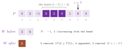
starts of the window in a deque \(W\) by increasing \(P\), whose head is
thus the best start (Algorithm 13.16 and
Figure 13.3): a new start \(x = i - L\) removes
from the tail the starts \(y\) with \(P[ y ] \ge P[ x ]\), which \(x\) dominates
for all the ends to come (it is as good and it stays in the window longer),
and the head is removed when it falls out of the window.
Algorithm 13.16. The segment of largest sum with the length in \([ L , U ]\), by the sliding minimum.
Lemma 13.4. After the step \(i\), the
starts in \(W\) lie in \([ i - U , i - L ]\) and have strictly increasing
prefix sums from the head to the tail, and the head is a start of least
\(P\) in that window; hence maxSumSegmentLength() finds a segment of
largest sum with the length in \([ L , U ]\) in \(O( n )\) time.
Proof. A start \(y\) removed from the tail by \(x > y\) has \(P[ y ] \ge P[ x ]\), and \(x\) stays in the window at least as long as \(y\); hence \(y\) is never needed again, and the starts left between the head and \(x\) have smaller prefix sums than \(x\). Hence, the head is the least of the starts left in the window, and no start removed was smaller than the one that removed it. Each start is appended once and removed at most once, which gives \(O( n )\) operations of the deque in all. \(\square\)
The longest segment of sum at least \(t\). The variant of Ferragina
2023, chapter 2 looks for the longest
segment whose sum is at least \(t\), e.g., the longest period with a gain of
at least \(t\). Let \(\ell\) be the length of the best segment found before the
end \(i\): only the starts \(x < L_i = i - \ell\) can beat it, and among them
only the leftmost minima of the prefix sums count (cf. Lemma 13.5), since a start \(y\) with
some \(x < y\) and \(P[ x ] \le P[ y ]\) is worse than \(x\) in both respects.
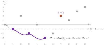
longestSegmentAtLeast() precomputes \(\mathit{LMin}[ x ]\), the leftmost
place of the minimum of \(P[ 0 .. x - 1 ]\), and walks the chain \(C_1 =
\mathit{LMin}[ L_i ]\), \(C_2 = \mathit{LMin}[ C_1 ]\), and so on, while the
sum \(P[ i ] - P[ C_j ]\) stays at least \(t\)
(Algorithm 13.17 and
Figure 13.4).
Algorithm 13.17. The longest segment of sum at least \(t\).
Lemma 13.5. The prefix sums of the chain
\(C_1 , C_2 , \ldots\) strictly increase as the chain moves left, and the
chain contains the leftmost minima of \(P\) to the left of \(L_i\); hence the
walk stops at the first start that fails, the last start that passes is
the best one for the end \(i\), and longestSegmentAtLeast() takes \(O( n )\)
time.
Proof. \(C_{j+1}\) is the leftmost minimum of \(P[ 0 .. C_j - 1 ]\), while \(C_j\) is the leftmost minimum of a longer prefix that contains it; hence \(P[ C_{j+1} ] > P[ C_j ]\), and the sums \(P[ i ] - P[ C_j ]\) decrease along the chain. A start of \([ 0 , L_i )\) that is not in the chain has a start of the chain to its left with a prefix sum not larger, which dominates it. At the end \(i\) the walk makes one failing step at most, and each step that passes moves the start to the left of the previous one; hence, the length found exceeds \(\ell\) by at least the number of the steps that pass. Since \(\ell \le n\), the steps that pass are at most \(n\) over all the ends, and the steps are \(O( n )\) in all, as is the computation of \(\mathit{LMin}\). \(\square\)
Clearly, the longest segment of average at least \(p / q\), \(q > 0\), is the same
problem on the items \(q D[ k ] - p\), whose segments have a sum not
negative if and only if the same segment of \(D\) has an average at least \(p /
q\) (longestSegmentAverageAtLeast(), which reports the sum of the segment
in \(D\)). Both measures of the regions rich in C and G of Ferragina 2023,
chapter 2 start from gcIndicator(),
which maps a DNA sequence to 1 for each C or G (in either case) and to 0
otherwise: the sum \(x - p \ell\) of the scores \(1 - p\) and \(-p\), and the
density \(x / \ell\), \(x\) being the count of C and G of a segment of length
\(\ell\).
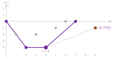
The segment of largest average. Among the segments of length at least
\(L\), the one of largest average is a question of slopes: the average of
\(D[ x .. i - 1 ]\) is the slope of the line from \(( x , P[ x ] )\) to \(( i ,
P[ i ] )\), and the best start \(x \le i - L\) for the end \(i\) is the point
where the tangent from \(( i , P[ i ] )\) touches the lower convex hull of
the points of the admissible starts. maxDensitySegment() keeps that hull
by the monotone chain as \(i\) grows (each new start is pushed after
popping the vertices where the chain does not turn left), and finds the
point of tangency by a binary search on the turns
(Algorithm 13.18 and
Figure 13.5), in \(O( n \log n )\) time. We remark that the
turns and the comparisons of the averages are cross products, i.e., the
algorithm makes no division, and it is exact on integers.
Algorithm 13.18. The segment of largest average with the length at least \(L\) (after Goldwasser, Kao and Lu 2005).
Lemma 13.6. For each end \(i\), a start of
largest average among the \(x \le i - L\) is a vertex of the lower convex
hull of the points \(( x , P[ x ] )\), the one where the tangent from \(( i ,
P[ i ] )\) touches it; hence maxDensitySegment() is correct, and it takes
\(O( n \log n )\) time.
Proof. The point \(( x , P[ x ] )\) that maximizes the slope towards \(( i , P[ i ] )\), a point to its right, is one such that no other point lies below the line through the two; such a point is on the lower hull. Along the hull, from left to right, the slopes towards \(( i , P[ i ] )\) first grow and then decrease, the largest being at the point of tangency, which is the first vertex whose edge to the next one turns away from \(( i , P[ i ] )\), and the binary search on the turns relies on this. Since the hull of the starts only grows on the right, the monotone chain pushes and pops each start at most once, in \(O( n )\) time in all; the binary searches cost \(O( \log n )\) each. \(\square\)
Goldwasser, Kao and Lu 2005 and Chung and Lu 2005 reach \(O( n )\) by walking the hull with a pointer that moves only forward, under a further argument, and also handle an upper bound on the length; we kept the binary search in the library, since it keeps the code short and exact on integers, at the price of a factor \(\log n\) that is usually "small".
All the functions of the section return a Segment< T >, but
gcIndicator() and maxSubarraySum():
// declarations of <ADS/algorithm/MaximumSegments.h>
//                  <ADS/algorithm/Subsequences.h>
template< class T >
Segment< T > maxSumSegmentCubic( const std::vector< T > & D );
template< class T >
Segment< T > maxSumSegmentQuadratic( const std::vector< T > & D );
template< class T >
Segment< T > maxSumSegment( const std::vector< T > & D );
template< class T >
Segment< T > maxSumSegmentPrefix( const std::vector< T > & D );
template< class T >
Segment< T > maxSumSegmentLength( const std::vector< T > & D , std::size_t L ,
                                  std::size_t U );
template< class T >
Segment< T > longestSegmentAtLeast( const std::vector< T > & D , T t );
template< class T >
Segment< T > longestSegmentAverageAtLeast( const std::vector< T > & D , T p ,
                                           T q );
template< class T >
Segment< T > maxDensitySegment( const std::vector< T > & D , std::size_t L );
std::vector< int > gcIndicator( const std::string & dna );
template< class T >
T maxSubarraySum( const std::vector< T > & A );
13.6 Sorts, sweeps and sliding windows¶
Most questions of SequenceQueries.h, and two of SequenceProblems.h, are
answered by a sort or by one scan faster than by the comparison of all the
pairs, each time by a property of the solutions that makes most pairs
irrelevant.
The smaller items on the right. For each place \(i\) of \(A[ 0 .. n - 1 ]\),
smallerToTheRight() counts the places \(j > i\) with \(A[ j ] < A[ i ]\), by
divide et impera (Montresor 2025, Esercizi
Divide-et-impera, exercise A3 of
14/06/2024). In fact, the algorithm is the bottom-up mergesort of the places, i.e.,
of a permutation \(P\) of \(0 , \ldots , n - 1\), by the items: the runs of
width \(w = 1 , 2 , 4 , \ldots\) are merged in pairs, and when an item of a
left run goes to the output, the items of the right run already output are
the smaller ones on its right in that run
(Algorithm 13.19).
Algorithm 13.19. The counts of the smaller items on the right, by mergesort.
Lemma 13.7. At the end, \(c[ i ]\) is the number of the places \(j > i\) with \(A[ j ] < A[ i ]\); the algorithm takes \(O( n \log n )\) time and \(O( n )\) space.
Proof. A place \(j > i\) with \(A[ j ] < A[ i ]\) is first in the same run as \(i\) after the merge of the run of \(i\), on the left, with the run of \(j\), on the right; there, \(j\) goes to the output before \(i\), since \(A[ j ] < A[ i ]\), and it is counted when \(i\) goes out. A place \(j\) with \(A[ j ] \ge A[ i ]\) goes out after \(i\), the left item going first on a tie, and it is not counted; the places to the left of \(i\) are never in a right run with respect to it. There are \(\lceil \log n \rceil\) widths, each costing \(O( n )\). \(\square\)
Note that the sum of the counts is the number of the inversions of \(A\), which the
contracts check as an audit against countInversions() of §12.4;
equal items do not count. A Fenwick tree on the ranks of the items gives
the same counts in \(O( n \log n )\) by a scan from the right (Fenwick
1994), with a tree of \(n\) counters in
place of the buffer of the merge.
Sliding windows. longestKDistinctRun() finds the first longest run
of consecutive items with at most \(k\) distinct values, by a window
\(S[ s .. e ]\) whose right end advances one place at a time and whose left
end advances while the window holds more than \(k\) values
(Algorithm 13.20). Here the counts of the values of
the window are kept in a std::map, which holds at most \(k + 1\) keys, and
since each end moves \(n\) times the time is \(O( n \log k )\) (somewhat more than
the \(O( n )\) expected time that a hash table would give).
longestDistinctSegment() of SequenceProblems.h is the case of the runs
with no value repeated (Montresor 2025, Esercizi Programmazione
dinamica, exercise A3 of 04/09/2020),
where the left end jumps past the last occurrence of the repeated value,
kept in a hash table of the last places, in \(\Theta( n )\) expected time.
Both are correct for the same reason, which we state for the first one
(Lemma 13.8).
Algorithm 13.20. The longest run with at most \(k\) distinct values, and the longest segment with no value repeated.
Lemma 13.8. After the step \(e\) of
longestKDistinctRun(), \(S[ s .. e ]\) is the longest run that ends in \(e\)
with at most \(k\) distinct values; hence the function returns the first
longest such run, in \(O( n \log k )\) time.
Proof. Call admissible a run with at most \(k\) distinct values; a run contained in an admissible one is admissible. Let \(s\) be the least admissible start for the end \(e - 1\) (by induction; \(s = 0\) before the first step). An admissible run \(S[ s' .. e ]\) with \(s' < s\) would contain the admissible run \(S[ s' .. e - 1 ]\), against the choice of \(s\); hence the least admissible start for \(e\) is at least \(s\), and the loop of lines 5 and 6, which advances \(s\) while \(S[ s .. e ]\) is not admissible, stops exactly at it. Line 7 keeps the first of the longest runs, since it replaces the best one only by a strictly longer one. Each of \(s\) and \(e\) advances at most \(n\) times, and each step costs \(O( \log k )\) on the map, which holds at most \(k + 1\) keys. \(\square\)
Sweeps of the line. largestGap() finds the longest stretch between
the first start and the last end of a set of closed intervals \([ a , b ]\)
that none of them covers, the first one on ties, by the sweep of the
intervals sorted by start (Algorithm 13.21):
the union of the intervals swept so far ends at the farthest end \(e\) met,
and a start \(a > e\) leaves the gap \(( e , a )\). This takes \(O( n \log n )\) time
for the sort; on integers, the lengths of the gaps are computed in the
unsigned type, where a gap from the least to the largest value of the
type does not overflow.
Algorithm 13.21. The largest gap of a set of intervals.
Lemma 13.9. largestGap() returns the
first of the longest open stretches between the first start and the last
end that no interval covers, or none if there is no such stretch.
Proof. Let the intervals be sorted by start. Before the interval \([ a , b ]\) is examined, \(e\) is the largest end among the intervals before it, whose union is a set of closed intervals contained in \(( -\infty , e ]\). If \(e < a\), no point of \(( e , a )\) is covered: the intervals before \([ a , b ]\) end by \(e\), and the others start at or after \(a\); the stretch is maximal, since \(e\) is covered and \(a\) is too. Conversely, let \(( x , y )\) be a maximal uncovered stretch between the first start and the last end; then \(x\) is the end of an interval, \(y\) the start of one, and when the sweep reaches the first interval that starts at \(y\), all the intervals that start before \(y\) end at or before \(x\) (one of them at \(x\)), so that \(e = x\) and line 5 compares the stretch. Since line 5 replaces the best stretch only by a strictly longer one, the first of the longest is kept. The sort costs \(O( n \log n )\), the rest \(O( n )\). \(\square\)
The water among the columns. trappingRainWater() computes the water
that columns of heights \(h_0 , \ldots , h_{n-1}\) hold after the rain, with
no walls outside them (Montresor 2025, Esercizi Programmazione
dinamica, exercise B2 of
20/07/2026). Over the column \(i\), the water reaches the lower of the two
highest columns on its sides, and the total is
which one can compute with two arrays of the maxima, or with a stack of the decreasing columns, in \(\Theta( n )\) time and space. Instead, the algorithm of the library uses two indices that move inwards from the ends, keeping the highest columns \(\ell\) and \(r\) met from the left and from the right (Algorithm 13.22), and it needs \(O( 1 )\) space: if \(\ell < r\), the level over the next column on the left is fixed by \(\ell\), since the maximum on its right is at least \(r > \ell\), and that column can be settled; symmetrically on the right.
Algorithm 13.22. The water held by the columns, by two indices.
Lemma 13.10. trappingRainWater()
returns (13.8), in \(\Theta( n )\) time and \(O( 1 )\) space.
Proof. Let \(\omega_c\) be the term of (13.8) of the column \(c\), which is 0 for \(c = 0\) and \(c = n - 1\). We show that, at each test of line 3, \(\ell = \max_{c \le i} h_c\), \(r = \max_{c \ge j} h_c\), and \(w\) is the sum of \(\omega_c\) over the columns \(0 < c \le i\) and \(j \le c < n - 1\), which are disjoint since \(i < j\); this holds at the start. Suppose that \(\ell < r\), and let \(c = i + 1\) and \(\ell' = \max\{ \ell , h_c \}\), the largest column on the left of \(c\), \(c\) included. The largest column on its right is at least \(r > \ell\) and at least \(h_c\), hence at least \(\ell'\), and therefore \(\omega_c = \ell' - h_c\), which line 5 adds. If \(c < j\), this keeps the invariant. If \(c = j\), the column is the column \(n - 1\) or one already counted, and the increment is 0 in both cases. In the first, \(r = h_c\) and the increment is \(\max\{ \ell , h_c \} - h_c = 0\). In the second, the last move of \(j\), onto \(c\), was made with \(r\) not above \(\ell\), which has not decreased since; hence \(r\) grew to \(h_c\) at that move, has not changed after it, and again \(r = h_c\). The case \(\ell \ge r\) is symmetric. The loop ends with \(i = j\), when \(w\) is the sum of all the \(\omega_c\), after \(n - 1\) steps of \(O( 1 )\). \(\square\)
The functions of the section are declared as follows; a run or a segment is returned as the pair of its first place and of its length:
// declarations of <ADS/algorithm/SequenceQueries.h>
//                  <ADS/optimization/SequenceProblems.h>
template< class T , class C = std::less<> >
std::vector< std::size_t > smallerToTheRight( const std::vector< T > & A ,
                                              C less = C() );
template< std::ranges::random_access_range R >
std::pair< std::size_t , std::size_t > longestKDistinctRun( const R & S ,
                                                           std::size_t k );
template< class T , class Hash = std::hash< T > >
std::pair< std::size_t , std::size_t >
longestDistinctSegment( const std::vector< T > & A );
template< class T >
 requires( std::is_arithmetic_v< T > && ! std::is_same_v< T , bool > )
std::optional< std::pair< T , T > >
largestGap( std::vector< std::pair< T , T > > I );
template< class T >
T trappingRainWater( const std::vector< T > & h );
13.7 Dynamic programming: the principle and the knapsack¶
A problem of optimization has optimal substructure when an optimal solution of an instance is made of a choice and of optimal solutions of the subproblems that the choice leaves, the subproblems being instances of the same problem on a part of the data (the first \(i\) objects, the keys from \(i\) to \(j\), the capacity \(c\)). A dynamic programming keeps the optimal value of each subproblem in a table, indexed by the parameters that name the subproblem (Montresor 2025, chapter 13).
Lemma 13.11 (the principle of optimality). If an optimal solution of an instance is made of a choice and of the solution of a subproblem that the choice leaves, then that solution is optimal for the subproblem.
Proof. A better solution of the subproblem, combined with the same choice, would give a better solution of the instance. \(\square\)
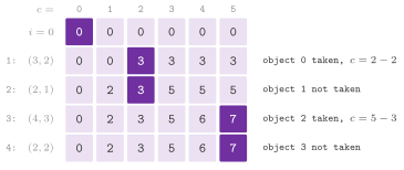
Hence, as we use it, the optimal value of an instance is the best, over the choices, of the value of the choice combined with the optimal value of what it leaves, i.e., a recurrence. In the 0-1 knapsack of Montresor 2025, §13.6 there are \(n\) objects of profits \(p_i\) and volumes \(v_i\), integers not negative, and a knapsack of capacity \(C\), and one looks for a set of objects of volume at most \(C\) and largest profit. Here the choice is whether to take the last object, and with \(\mathit{DP}[ i ][ c ]\) the best profit of the first \(i\) objects in the capacity \(c\) one has
with \(\mathit{DP}[ i - 1 ][ c - v_{i-1} ] = -\infty\) when \(v_{i-1} > c\) (the objects numbered from 0). Since the subproblems of (13.9) overlap, i.e., the same one is reached by many sequences of choices, the recursion written as it stands takes exponential time; the dynamic programming instead solves each of them once, either bottom up, filling the table in an order in which each entry comes after those it reads, or top down, by the recursion with a memo of the values already found.
knapsack() fills the table bottom up, row by row, and reads the set back
from the table by retracing the choices that gave each optimum: the object
\(i - 1\) is in the set when \(\mathit{DP}[ i ][ c ] \ne \mathit{DP}[ i - 1 ][
c ]\), and then the capacity drops by its volume
(Algorithm 13.23 and
Figure 13.6). Volumes may also be 0, and
the column \(c = 0\) is therefore filled by the same maximum instead of being
set to 0, as it is in the book.
Algorithm 13.23. The 0-1 knapsack, bottom up (Montresor 2025, §13.6).
knapsackMemo() (zaino() in the book, kept as an alias) is the
memoization (Algorithm 13.24), which solves only the subproblems that the recursion from \(( n , C )\)
reaches. Its memo is a hash table per object (a ChainedHashTable of
§7.4, of key \(c\)) instead of a table of \(( n + 1 ) ( C + 1 )\) places,
whose initialization alone would cost \(\Theta( n C )\); hence any capacity
up to the largest long is allowed, which knapsack() cannot do. One
table per object, instead of one table of key \(i ( C + 1 ) + c\), avoids the
overflow of that key for large capacities. If a pointer solved is given,
the function counts there the subproblems that it solves, which a test uses
to compare them with the \(n C\) entries of the full table.
Algorithm 13.24. The 0-1 knapsack by memoization (Montresor 2025, §13.6), called as \(\mathrm{knapsackMemo}( n , C )\).
Lemma 13.12. knapsack() returns a set of
largest profit among those of volume at most \(C\), in \(\Theta( n C )\) time
and space; knapsackMemo() returns its profit in \(O( \min\{ n C , 2^n \} )\) expected time and
space.
Proof. The correctness of (13.9) is Lemma 13.11
with the two choices for the last object, and the reading back retraces a
choice that attains each optimum. Also, the table has \(( n + 1 ) ( C + 1 )\)
entries, each computed in \(O( 1 )\). knapsackMemo() solves each pair \(( i , c )\)
once, and the pairs reached are at most \(n ( C + 1 )\) and at most \(2^{n+1}\),
since the recursion branches in two; each costs \(O( 1 )\) expected time of
the hash table. \(\square\)
We remark that the bound \(\Theta( n C )\) is pseudopolynomial: it is polynomial in the value \(C\), but \(C\) takes only \(\log C\) bits of the input, and the bound is exponential in the size of the input. This is not a defect of the algorithm, since the decision version of the 0-1 knapsack is NP-complete (chapter 20). In general, the cost of a dynamic programming is the number of its subproblems times the cost of one recurrence. Furthermore, the subproblems and their dependences form a directed acyclic graph, and a dynamic programming may be read as a longest or a shortest path in it, which is how the problems on a row of houses of §13.9 read. Table 13.4 groups the recurrences of the area by the shape of their subproblems, which decides the size of the table and therefore the cost.
Table 13.4. The dynamic programmings of
ADS/optimization and ADS/algorithm, by the shape of the subproblems;
\(C\) is a capacity or an amount, \(k\) a number of parts, of colors or of
transactions, and \(m \times n\) the size of a grid.
| Subproblems | Functions | Table kept | Time |
|---|---|---|---|
| a prefix and a capacity | knapsack(), knapsackMemo(), subsetSumCount() |
\(n \times C\), or one row | \(\Theta( n C )\) |
| a capacity, items in unlimited supply | unboundedKnapsack(), rodCutting(), minValueExactWeight(), coinChangeWays(), optimalChange() |
one row of \(C + 1\) | \(\Theta( n C )\) |
| a prefix of a sequence | maxinterval(), maxNonAdjacentSum(), paintHouses(), maxProfit() |
\(n\) (times the states) | \(O( n )\) to \(O( n k )\) |
| a prefix, the best predecessor among all | lis(), largestDivisibleSubset(), longestChainSubsequence() |
\(n\) | \(\Theta( n^2 )\) |
| a range \([ i , j )\) | coinsInALine(), optimalSearchTree() |
\(n \times n\), or one row | \(\Theta( n^2 )\) |
| a prefix and a number of parts | linearPartition() |
\(k \times n\) | \(O( k n^2 )\) |
| a cell of a grid | largestSquare(), countLatticePaths() |
one row of \(n\) | \(\Theta( m n )\) |
Both functions take the profits and the volumes as vectors of long;
knapsack() returns the best profit with the places of the objects
taken:
// declarations of <ADS/optimization/Knapsack.h>
std::pair< long , std::vector< std::size_t > >
knapsack( const std::vector< long > & p , const std::vector< long > & v ,
          long C );
long knapsackMemo( const std::vector< long > & p ,
                   const std::vector< long > & v , long C ,
                   long * solved = nullptr );
long zaino( const std::vector< long > & p , const std::vector< long > & v ,
            long C , long * solved = nullptr );
13.8 Dynamic programming on a capacity¶
In KnapsackVariants.h and CoinChange.h, the relatives of the knapsack
have one parameter, the capacity or the amount, and items in unlimited
supply (but for subsetSumCount()); their tables are a single row of \(C +
1\) entries, each computed from the entries of smaller capacity
(Montresor 2025, Esercizi Programmazione
dinamica; Martello and Toth
1990). In the unbounded knapsack
(unboundedKnapsack()) the objects of profits \(p\) and volumes \(v > 0\) can
be taken any number of times, and
where the first term leaves a unit of the capacity empty; the function
records the last object added for each capacity, and reads the copies of
each object back from \(C\) (Algorithm 13.25),
in \(O( n C )\) time and \(O( C )\) space. Similarly, the cut of a rod of length \(L\)
(rodCutting(), exercise B4 of 01/02/2012 in the book), with
\(\mathit{price}[ t - 1 ]\) the price of a piece of length \(t \le m\), is the
same recurrence with the lengths \(1 , \ldots , m\) as the volumes and no
unit left empty, \(R[ l ] = \max_{1 \le t \le \min( l , m )}
\mathit{price}[ t - 1 ] + R[ l - t ]\), in \(O( L m )\) time.
Algorithm 13.25. The unbounded knapsack and the cut of a rod.
Lemma 13.13. \(P[ c ]\) of (13.10) is the
largest profit of a multiset of the objects of total volume at most \(c\);
\(R[ l ]\) is the largest price of the cut of a rod of length \(l\) into
pieces of lengths at most \(m\); \(N[ c ]\) of optimalChange() is the fewest
coins that pay exactly \(c\), and \(D[ x ]\) of minValueExactWeight() the
least value of coins that weigh exactly \(x\) (\(\textbf{nil}\) if none
does).
Proof. By induction on \(c\). A multiset of volume at most \(c\) either has volume at most \(c - 1\), and its profit is at most \(P[ c - 1 ]\), or it has volume exactly \(c\) and contains some object \(i\), whose removal leaves a multiset of volume at most \(c - v_i\) and profit at most \(P[ c - v_i ]\), since \(v_i > 0\); conversely each term of (13.10) is the profit of such a multiset, built from one that attains the term. The other three are the same argument with the volume exact: the last piece, or a coin of the change, of size \(t\) leaves an exact subproblem of size \(l - t\) (or \(c - d\)), which is optimal by Lemma 13.11, and an amount that no coin leaves reachable stays \(\textbf{nil}\). Each entry compares at most \(n\) (or \(m\)) terms. \(\square\)
Problems of change minimize the same kind of
recurrence over the amounts that are reached with no remainder.
minValueExactWeight() (exercise B4 of 02/02/2015) finds the least value
of coins of weights \(w\) and values \(v\), in unlimited supply, that weigh
exactly \(W\), with \(D[ x ] = \textbf{nil}\) for a weight that no coins make;
with all the values 1 it is the fewest coins of the change, which
optimalChange() of CoinChange.h computes as \(N[ c ] = 1 + \min_{d \le c}
N[ c - d ]\) in \(O( n c )\) time (Algorithm 13.26).
§13.11 compares it with the greedy choice.
Algorithm 13.26. The least value of the coins of a given weight, and the fewest coins of the change.
Counting. The number of ways of paying \(T\) with coins of the given
values, in unlimited supply and with the order not counting
(coinChangeWays(), exercise B3 of 31/05/2012), and the number of
subsets of the places of \(A\) of sum \(k\) (subsetSumCount()), are both
sums over the same table (cf. (13.9)), \(N[ x ] \mathrel{+}= N[ x - d ]\); they differ in
the order in which the table is filled, and that order decides what they
count (Algorithm 13.27).
Algorithm 13.27. The ways of paying an amount, and the subsets of a given sum.
Lemma 13.14. In coinChangeWays(), after
the coins \(d_1 , \ldots , d_j\) have entered, \(N[ x ]\) is the number of
multisets of those coins of sum \(x\); in subsetSumCount(), after the
items \(a_1 , \ldots , a_j\), \(N[ x ]\) is the number of the subsets of their
places of sum \(x\). Both take \(O( n T )\), resp. \(O( n k )\), time and \(O( T
)\), resp. \(O( k )\), space.
Proof. By induction on \(j\). In coinChangeWays() the amounts go up, so
that \(N[ x - d_j ]\) has already been updated for the coin \(d_j\) and counts
the multisets that use \(d_j\) any number of times; hence \(N[ x ]\) adds to
the multisets without \(d_j\) those with at least one more copy of it, each
multiset being counted once, with its coins in the order in which they
entered. In subsetSumCount() the sums go down, and therefore \(N[ x - a_j ]\)
still counts the subsets of the first \(j - 1\) items only, and \(a_j\) is
used at most once; this is the row of (13.9) kept in place. \(\square\)
These counts are the coefficients of the generating functions
\(\prod_d ( 1 - z^d )^{-1}\) and \(\prod_i ( 1 + z^{a_i} )\), and they may grow
"quickly"; the type of the counters is a parameter, std::uint64_t by
default. Also, the bounded knapsack, in which the object \(i\) is available \(b_i\)
times, reduces to the 0-1 one by splitting \(b_i\) into powers of two
(Martello and Toth 1990).
Sums of squares. minimumSquares() finds the fewest squares of
positive integers that sum to \(n\). A dynamic programming \(S[ i ] = 1 +
\min_{t^2 \le i} S[ i - t^2 ]\) asked by the exercise B4 of 26/01/2016
takes \(\Theta( n \sqrt n )\) time; number theory answers in
\(O( \sqrt n \log n )\)
(Algorithm 13.28), since the answer is at most
4 by the four-square theorem of Lagrange, it is 4 exactly when \(n = 4^a ( 8
b + 7 )\) by the three-square theorem of Legendre, and the cases 1 and 2
are found by testing the squares (Rabin and Shallit
1986, who also find the squares
themselves). To test a square, the function finds the integer square root by a binary
search on its bits, which never squares a number larger than \(n\), and
therefore never overflows.
Algorithm 13.28. The fewest squares that sum to \(n\).
Lemma 13.15. minimumSquares() returns
the fewest squares of positive integers that sum to \(n\), in
\(O( \sqrt n \log n )\) time.
Proof. Every \(n \ge 0\) is a sum of four squares (Lagrange), and \(n\) is a sum of three squares if and only if it is not of the form \(4^a ( 8 b + 7 )\) (Legendre); both are classic results of number theory, for which we refer to Rabin and Shallit 1986. Hence the answer is 1 if \(n\) is a square (line 3), 4 if and only if line 5 returns, 2 if and only if some \(n - t^2\), \(1 \le t \le \lfloor \sqrt n \rfloor\), is a square (lines 6 and 7; \(t^2 = n\) was excluded at line 3), and 3 otherwise. Each test of a square is a binary search of \(O( \log n )\) steps on the bits of the root, and line 6 makes at most \(\sqrt n\) of them. \(\square\)
The functions of the section are declared as follows, the counters
being of the type C:
// declarations of <ADS/optimization/KnapsackVariants.h>
//                  <ADS/optimization/CoinChange.h>
template< class T , class V >
std::pair< T , std::vector< std::size_t > >
unboundedKnapsack( const std::vector< T > & p , const std::vector< V > & v ,
                   V C );
template< class T >
std::pair< T , std::vector< std::size_t > >
rodCutting( const std::vector< T > & price , std::size_t L );
template< class T , class V >
std::optional< T > minValueExactWeight( const std::vector< V > & w ,
                                        const std::vector< T > & v , V W );
std::optional< long > optimalChange( const std::vector< long > & coins ,
                                     long c );
template< class C = std::uint64_t , class V >
C coinChangeWays( const std::vector< V > & coins , V T );
template< class C = std::uint64_t , class V >
C subsetSumCount( const std::vector< V > & A , V k );
int minimumSquares( std::int64_t n );
13.9 Dynamic programming on a prefix¶
When the data form a sequence and the choice concerns its last item, the subproblems are the prefixes, and the table has one entry per prefix (times the states of the last item, if any). Its cost is then decided by the number of the predecessors that the recurrence compares, and a structure on the predecessors may give the best of them faster than the scan.
Weighted intervals. Among \(n\) intervals \([ a_i , b_i )\), open on the right, of weights \(w_i \ge 0\), the problem of Montresor 2025, §13.2 looks for a set of disjoint ones of largest weight. With the intervals numbered from 1 by increasing right end and \(\mathit{pred}[ i ]\) the largest \(j < i\) whose interval ends at or before the start of the interval \(i\) (0 if none),
since an optimal set either leaves the interval \(i\) out, or contains it
together with an optimal set of the intervals that end before it starts,
which are the first \(\mathit{pred}[ i ]\) ones. maxinterval() takes the
intervals as WeightedIntervals, of fields a, b and w, and computes all
the predecessors by one scan of the \(2 n\) ends sorted, a right end coming
before a left one equal to it (the intervals are open on the right, and an
interval that ends at \(x\) is compatible with one that starts at \(x\)): a
left end of \(i\) sets \(\mathit{pred}[ i ]\) to the largest interval whose
right end has been met (Algorithm 13.29).
This takes \(O( n \log n )\) time for the sorts and \(O( n )\) for the rest; the
set is read back from \(\mathit{DP}[ n ]\), the interval \(i\) being taken when
it gives a strictly larger weight.
Algorithm 13.29. The independent set of weighted intervals (Montresor 2025, §13.2).
Rows of houses. maxNonAdjacentSum() finds the largest sum of items
of \(A\) no two of them adjacent (the donations of houses no two of which
are neighbours, exercise B3 of 17/06/2013 in the book), i.e., the maximum
weight independent set of a path: \(D[ i ] = \max( D[ i - 1 ] , D[ i - 2 ] +
A_{i-1} )\), \(D[ 0 ] = D[ -1 ] = 0\), which is (13.11) on the unit intervals
\([ i , i + 2 )\). It keeps the last two entries, in \(\Theta( n )\) time and
\(O( 1 )\) space, while nonAdjacentSelection() keeps the table and reads
the places back, an item being taken only if it makes the sum larger.
paintHouses() (exercise B3 of 02/02/2026) paints a row of \(n\) houses with
\(k\) colors, \(\mathit{cost}[ h ][ c ]\) for the house \(h\) of the color \(c\)
and adjacent houses of different colors:
\(O( n k^2 )\) as written. Keeping, of each row, its least entry, its color and its second least entry, the minimum over \(q \ne c\) is one of the two, and the time falls to \(O( n k )\) (Algorithm 13.30); the colors are read back from the table of \(O( n k )\) space. Both are shortest or longest paths in the graph of the states (house, choice), and generalize to a tree of houses by the same recurrence on the children (Kleinberg and Tardos 2005, §6.1).
Algorithm 13.30. The largest sum of items no two of them adjacent, and the cheapest painting of a row of houses.
Lemma 13.16. (13.11) gives the largest weight of a set of disjoint intervals among the first \(i\), the scan of the sorted ends gives \(\mathit{pred}\), and (13.12) the least cost of a painting of the first \(h + 1\) houses with the house \(h\) of the color \(c\); in Algorithm 13.30 the minimum over \(q \ne c\) is the entry of the color \(s\) when \(c = b\) and that of \(b\) otherwise.
Proof. The intervals that end at or before \(a_i\) are a prefix of the
order by right end, of length \(\mathit{pred}[ i ]\), and when the left end
of \(i\) is met in the scan, the right ends met are exactly those not above
\(a_i\) (a right end equal to \(a_i\) comes first). An optimal set of the first
\(i\) intervals either leaves out the interval \(i\), or contains it with a set
of intervals disjoint from it, i.e., among the first \(\mathit{pred}[ i ]\),
which is optimal by Lemma 13.11; this gives
(13.11), and the case of maxNonAdjacentSum() is that of the unit
intervals. In the same way, a painting of the houses up to \(h\) with \(h\) of
the color \(c\) is one of the houses up to \(h - 1\) with \(h - 1\) of a color
\(q \ne c\), which gives (13.12). Finally, if \(c\) is not the color \(b\) of
the least entry of the row \(h - 1\), that entry is the minimum over
\(q \ne c\); otherwise the minimum over the other colors is the second least
entry, of the color \(s\). \(\square\)
Transactions on a stock. Given the prices of a stock on \(n\) days,
maxProfit() finds the largest gain of at most \(k\) transactions, each one
buying on a day and selling on a later one, with no two of them
overlapping, \(b_1 < s_1 < b_2 < \cdots < b_k < s_k\) (exercise B3 of
12/01/2026 in the book). Its scan of the days keeps, for each \(l \le k\),
the best balance \(\mathit{free}[ l ]\) with \(l\) transactions closed and no
stock in hand, and the best balance \(\mathit{hold}[ l ]\) with the stock of
the \(l\)-th transaction in hand; on a day of price \(x\),
with \(l\) going down from \(k\) to 1 (Algorithm 13.31).
Note that the order matters: \(\mathit{free}[ l ]\) reads \(\mathit{hold}[ l ]\) before
it is updated on the same day, and \(\mathit{hold}[ l ]\) reads
\(\mathit{free}[ l - 1 ]\) before it is, and each sale and the next
purchase therefore fall on distinct days. This takes \(O( n k )\) time and \(O( k
)\) space, against the \(O( k n^2 )\) of the table on the day of the last sale
written in the text of the exercise. For \(k \ge n / 2\) the bound on the
transactions does not bind, and the answer is the sum of the positive
differences of consecutive prices, in \(O( n )\); for \(k = 1\) it is the
largest difference \(x_s - x_b\), \(s > b\), i.e., the segment of largest sum
of the differences (§13.5). With exactly \(k\)
transactions (maxProfitExactly()) the answer may be negative, and there
is none for \(n < 2 k\); the balances not reachable are kept as empty
std::optionals, which lose every maximum.
Algorithm 13.31. The largest gain of at most \(k\) transactions, and of exactly \(k\).
Lemma 13.17. Let \(\mathit{free}[ 0 ] = 0\)
and the other balances be \(-\infty\) (an empty std::optional) at the
start. Then, after the day \(d\), \(\mathit{free}[ l ]\) is the largest balance of
\(l\) transactions \(b_1 < s_1 < \cdots < b_l < s_l \le d\), and
\(\mathit{hold}[ l ]\) that of \(l - 1\) such transactions followed by a
purchase \(b_l \le d\), \(b_l > s_{l-1}\); hence maxProfit() and
maxProfitExactly() are correct, in \(O( n k )\) time and \(O( k )\) space.
Proof. By induction on \(d\). A sequence of \(l\) transactions closed by the day \(d\) either makes no sale on the day \(d\), and its best balance is the old \(\mathit{free}[ l ]\), or sells on the day \(d\) the stock bought on a day \(b_l < d\), and its best balance is \(x\) plus the \(\mathit{hold}[ l ]\) of the day \(d - 1\); this is the value that (13.13) reads, since \(\mathit{hold}[ l ]\) is updated after \(\mathit{free}[ l ]\). Similarly, a purchase on the day \(d\) follows \(l - 1\) sales on days before \(d\), whose best balance is the \(\mathit{free}[ l - 1 ]\) of the day \(d - 1\), still unchanged when \(\mathit{hold}[ l ]\) reads it, since \(l\) goes down. For \(k \ge n / 2\), a transaction gains \(x_s - x_b\), the sum of the differences of consecutive prices from \(b\) to \(s\), and therefore no set of transactions gains more than the sum of the positive differences. This sum is gained by one transaction per maximal run of days of rising price. These runs are disjoint and of at least two days each, and hence at most \(n / 2 \le k\). \(\square\)
Increasing subsequences. The longest increasing subsequence of \(A[ 0
.. n - 1 ]\) (Montresor 2025, exercise 13.6)
is a recurrence over all the predecessors: with \(L[ i ]\) the length of the
longest one that ends in \(A[ i ]\), \(L[ i ] = 1 + \max\{ L[ j ] : j < i ,
A[ j ] < A[ i ] \}\), and lis() finds one in \(\Theta( n^2 )\) time,
reading it back from the predecessors
(Algorithm 13.32). lisLength() finds its
length in \(O( n \log n )\) (Fredman 1975)
by keeping, instead of the lengths of the subsequences that end at each
place, the least item that ends one of each length.
Algorithm 13.32. The longest increasing subsequence, in \(\Theta( n^2 )\) and in \(O( n \log n )\).
Lemma 13.18. After each item, for each \(\ell\),
and \(\mathit{tails}\) is strictly increasing; hence its size at the end is the length of a longest increasing subsequence, found in \(O( n \log n )\) time.
Proof. A subsequence of \(\ell + 2\) items ends with an item larger than the end of its first \(\ell + 1\) items, and therefore \(\mathit{tails}\) is strictly increasing. A new item \(a\) extends the subsequences whose last item is below \(a\), the longest of which has \(\ell\) items, \(\ell\) being the first place with \(\mathit{tails}[ \ell ] \ge a\) (found by binary search); it gives a subsequence of \(\ell + 1\) items that ends with \(a \le \mathit{tails}[ \ell ]\), and it changes no other entry of (13.14). \(\square\)
One can use the same recurrence over all the predecessors for the problems of
SequenceProblems.h in which the order between two items is not total
(Algorithm 13.33).
longestChainSubsequence() (exercise B4 of 06/06/2011) finds the longest
subsequence of \(S\) each item of which precedes the next in a strict
partial order, e.g., boxes each fitting in the next, with \(\Theta( n^2 )\)
comparisons; when the boxes may be sorted and rotated it is the box
stacking problem, i.e., the longest path in the graph of the dominance.
largestDivisibleSubset() (exercise B3 of 28/08/2026) finds the largest
subset of distinct positive integers in which, of any two, one divides the
other: on the items sorted, such a subset is a chain in the order of
divisibility, and by the transitivity of divisibility a chain needs only
that each item divide the next, which gives \(L[ i ] = 1 + \max\{ L[ j ] : j <
i , a_j \mid a_i \}\), in \(\Theta( n^2 )\) time. When the order is total and
the measure a weight, a structure on the predecessors helps again:
maxSumIncreasingSubsequence() (exercise B3 of 16/06/2021) computes \(D[ i
] = a_i + \max\{ D[ j ] : j < i , a_j < a_i \}\), the heaviest increasing
subsequence with the items as weights (Jacobson and Vo
1992), taking the maximum over the
smaller values from a Fenwick tree of the prefix maxima on the ranks of the
values, in \(O( n \log n )\) time instead of \(\Theta( n^2 )\) (cf. Lemma 13.18, whose bound it matches). A negative item
starts no subsequence, since the empty one, of sum 0, is better.
Algorithm 13.33. The longest chain in a partial order, the largest divisible subset, and the heaviest increasing subsequence.
Lemma 13.19. In lis() and
longestChainSubsequence(), \(L[ i ]\) is the length of a longest
subsequence that ends in the item \(i\) and each item of which precedes the
next; in largestDivisibleSubset(), on the items sorted, \(L[ i ]\) is the
size of a largest divisible subset whose largest item is \(a_i\); in
maxSumIncreasingSubsequence(), \(D[ i ]\) is the largest sum of an
increasing subsequence that ends in \(a_i\).
Proof. A longest subsequence that ends in the item \(i\) is the item \(i\)
alone, or a subsequence that ends in some \(j < i\) preceding it, followed by
\(i\), and the former is then longest among those that end in \(j\) by
Lemma 13.11; the maximum over \(j\) is thus
\(L[ i ]\), and the same holds for the sums. For the divisible subsets, a
set of distinct positive integers, sorted, in which each item divides the
next, is divisible, since divisibility is transitive; conversely, in a
divisible set sorted the smaller of two consecutive items divides the
larger. Hence the divisible subsets are the chains of the order "divides"
on the sorted items, and the first claim applies. Finally, the Fenwick
tree of maxSumIncreasingSubsequence() holds, at the rank \(r\) of a value,
the largest \(D[ j ]\) of the items \(j < i\) of that value, and its query of
the prefix of the ranks below that of \(a_i\) gives the maximum over the
smaller values in \(O( \log n )\). \(\square\)
The functions of the section are declared as follows; those that return a pair give the optimum together with the places, or the colors, that attain it:
// declarations of <ADS/optimization/WeightedIntervals.h>
//                  <ADS/optimization/HouseProblems.h>
//                  <ADS/optimization/StockTrading.h>
//                  <ADS/algorithm/Subsequences.h>
//                  <ADS/optimization/SequenceProblems.h>
template< class W >
std::pair< std::vector< std::size_t > , W >
maxinterval( const std::vector< WeightedInterval< W > > & I );
template< class T >
T maxNonAdjacentSum( const std::vector< T > & A );
template< class T >
std::pair< T , std::vector< std::size_t > >
nonAdjacentSelection( const std::vector< T > & A );
template< class T >
std::pair< T , std::vector< std::size_t > >
paintHouses( const std::vector< std::vector< T > > & cost );
template< class T >
T maxProfit( const std::vector< T > & prices , std::size_t k );
template< class T >
std::optional< T > maxProfitExactly( const std::vector< T > & prices ,
                                     std::size_t k );
template< class T >
std::vector< T > lis( const std::vector< T > & A );
template< class T >
std::size_t lisLength( const std::vector< T > & A );
template< class T , class Less >
std::vector< std::size_t > longestChainSubsequence( const std::vector< T > & S ,
                                                    Less less );
template< std::integral T >
std::vector< T > largestDivisibleSubset( std::vector< T > A );
template< class T >
T maxSumIncreasingSubsequence( const std::vector< T > & A );
13.10 Dynamic programming on a range and on a grid¶
When a choice splits the data into a left and a right part, as usually happens with trees, the subproblems are the ranges \([ i , j )\), \(O( n^2 )\) of them, and the table is filled by increasing length of the range.
A game. In the game of the coins in a line, \(n\) coins of values \(V_0 ,
\ldots , V_{n-1}\) lie in a row, and two players take in turn the first or
the last coin left, each one to get the most (exercise B4 of 22/07/2013 in
the book; Winkler 2004).
coinsInALine() computes the most that the first player can be sure of,
against any play of the other. With \(D[ i ][ j ]\) the largest difference
between the coins of the player to move and those of the other on \(V[ i ..
j - 1 ]\),
since after a move the other player becomes the player to move on the coins left, and the first player gets \(( S + D[ 0 ][ n ] ) / 2\), \(S\) being the sum of the coins. Filled by increasing length, the table keeps one row, the entry \(D[ i ]\) holding \(D[ i ][ i + h ]\) for the current length \(h\) (Algorithm 13.34), in \(\Theta( n^2 )\) time and \(\Theta( n )\) space; the values may be negative. In other words, the scheme is the minimax on the ranges, and the form with two moves ahead, \(M[ i ][ j ] = \max( V_i + \min( M[ i + 2 ][ j ] , M[ i + 1 ][ j - 1 ] ) , \ldots )\), gives the same value. For \(n\) even the first player never loses, since the coins of even places and those of odd places can each be taken all by the first player, who chooses the larger set; this strategy, though, is not optimal in general.
Algorithm 13.34. The game of the coins in a line.
Lemma 13.20. (13.15) gives the largest difference that the player to move on \(V[ i .. j - 1 ]\) can be sure of against any play of the other; the first player gets \(( S + D[ 0 ][ n ] ) / 2\), and for \(n\) even at least \(S / 2\).
Proof. By induction on \(j - i\), the case \(i = j\) being clear. If the player to move takes \(V_i\), the other becomes the player to move on \(V[ i + 1 .. j - 1 ]\) and can be sure of the difference \(D[ i + 1 ][ j ]\), and no more, against the best play of the first; the first thus gets \(V_i - D[ i + 1 ][ j ]\), and symmetrically for \(V_{j-1}\), and the better of the two moves gives (13.15). With \(x\) and \(y\) the coins of the two players, \(x - y = D[ 0 ][ n ]\) and \(x + y = S\). For \(n\) even, let the first player fix a parity. Before each of its moves the coins left are a run of even length, whose two ends have places of different parity, and it takes the end of the parity fixed; the run left has odd length and both its ends of the other parity, one of which the other player must take. Hence the first player can take all the coins of the even places, or all those of the odd places, and the larger of the two sums is at least \(S / 2\); the optimal play gets at least as much. \(\square\)
Optimal binary search trees. The keys \(0 , \ldots , n - 1\) are searched with the weights \(p_i\) (frequencies or probabilities), and the gaps between them, the unsuccessful searches, with the weights \(q_0 , \ldots , q_n\); the optimal binary search tree is the one of least weighted path length \(\sum_i p_i ( d_i + 1 ) + \sum_j q_j d'_j\), with \(d_i\) the depth of the key \(i\), \(d'_j\) that of the external node \(j\), and the root at depth 0 (Knuth 1971). With \(W( i , j ) = \sum_{i \le l < j} p_l + \sum_{i \le l \le j} q_l\), the cost of the keys \(i , \ldots , j - 1\) is \(C[ i ][ i ] = 0\) and
since all the nodes of the tree go one level deeper under the root \(r\). There are \(O( n )\) choices for each of the \(O( n^2 )\) ranges, i.e., \(O( n^3 )\) time as written; however, the bound falls by the following property.
Theorem 13.4 (Knuth; Yao). If \(W\) is monotone on the inclusion of the ranges and satisfies the quadrangle inequality \(W( i , j ) + W( i' , j' ) \le W( i' , j ) + W( i , j' )\) for \(i \le i' \le j \le j'\), then the largest best root \(R[ i ][ j ]\) of (13.16) satisfies
This theorem was proved by Knuth 1971
for the search trees, and derived by Yao
1980 from the quadrangle inequality, which
the weights of the keys and of the gaps satisfy with equality (and \(W\) is
monotone, the weights being not negative, as the precondition of
optimalSearchTree() requires); we refer to
the latter for the proof (which is somewhat long), which shows first that \(C\) inherits the
quadrangle inequality from \(W\).
Lemma 13.21. With the roots looked for
in the ranges (13.17), optimalSearchTree() takes \(O( n^2 )\) time and
space.
Proof. For the ranges of one length \(h\), the candidates of the range \([ i , i + h )\) are \(R[ i + 1 ][ i + h ] - R[ i ][ i + h - 1 ] + 1\), and their sum over \(i\) telescopes to \(O( n )\); the \(n\) lengths cost \(O( n^2 )\) in all, and the tables \(C\) and \(R\) have \(( n + 1 )^2\) entries. \(\square\)
Algorithm 13.35. The optimal binary search tree, with the bound of Knuth on the roots (exercise B4 of 11/01/2012 of Montresor 2025, with the gaps and the bound beyond the book), and its form with the gaps of weight 0.
In the code, the loop keeps the largest best root, the one of (13.17), by preferring a later candidate on a tie; the tree is then built from \(R[ 0 ][ n ]\) down, as the children of each key, and the contracts check, as an audit, that its symmetric visit is \(0 , \ldots , n - 1\) and that its weighted path length is the cost found. In the literature, Hu and Tucker 1971 and Garsia and Wachs 1977 build in \(O( n \log n )\) the optimal alphabetic tree, where only the \(q_j\) count (the keys in the leaves); a tree within a constant of the optimum comes in \(O( n )\) from the weight-balancing rule of Mehlhorn 1975; and the splay trees of §8.8 are within a constant of the optimal static tree without knowing the weights.
Partitions of a sequence. The linear partition problem (also the
painter's partition, or the bottleneck partition of a chain) splits the
items \(A[ 0 .. n - 1 ]\) into \(k\) contiguous parts in which the largest sum
of a part is the least, e.g., \(n\) boards of lengths \(A_i\) to be painted by
\(k\) painters, each one a block of consecutive boards, in the least time
(Skiena 2020, §10.7).
linearPartition() (exercise B4 of 05/06/2014) solves it for items of any
sign and exactly \(k\) nonempty parts, by the dynamic programming on the
prefix sums \(S\),
with the best cut kept for each entry, in \(O( k n^2 )\) time and \(O( k n )\)
space (Algorithm 13.36). painterPartition()
solves it for integer items not negative and at most \(k\) parts by a
binary search on the answer \(x\) (cf. Lemma 13.23), each candidate checked by the greedy
fits(), which closes a part only when the next item does not fit in it.
Algorithm 13.36. The linear partition by dynamic programming, and the painter's partition by a binary search on the answer.
Lemma 13.22. \(D[ t ][ i ]\) of (13.18) is
the least largest sum of a split of \(A[ 0 .. i - 1 ]\) into \(t\) nonempty
contiguous parts, and linearPartition() takes \(O( k n^2 )\) time.
Proof. In a split into \(t \ge 2\) parts, the last part is \(A[ j .. i - 1 ]\) for some \(j \in [ t - 1 , i )\), since the first \(t - 1\) parts need \(t - 1\) items at least; its largest sum is the larger of \(S[ i ] - S[ j ]\) and of the largest sum of the other \(t - 1\) parts, and the split of \(A[ 0 .. j - 1 ]\) may be taken optimal, which can only lower the maximum. Hence (13.18) by induction on \(t\), with \(D[ 1 ][ i ] = S[ i ]\) for one part. Each of the \(k n\) entries compares at most \(n\) cuts. \(\square\)
Lemma 13.23. For items not negative, the
greedy fits() uses the fewest parts of sum at most \(x\); hence \(x\) is
feasible if and only if it needs at most \(k\) parts, and painterPartition()
takes \(O( n \log \sum_i A_i )\) time and \(O( 1 )\) space.
Proof. By induction on the parts, the \(j\)-th part of the greedy ends no
earlier than the \(j\)-th part of any split of sums at most \(x\), since it
starts no later and takes items while they fit. Feasibility is monotone in
\(x\), and the binary search between \(\max_i A_i\) and \(\sum_i A_i\) makes
\(O( \log \sum_i A_i )\) calls of fits(), each of \(O( n )\) time. \(\square\)
With items not negative and \(k \le n\), at most \(k\) parts and exactly \(k\) nonempty ones give the same value, since a part can be split without raising the largest sum. In the literature, the problem on a chain is solved in \(O( n )\) time for \(k\) fixed, and in \(O( n + k^2 \log^2 n )\) in general, by a parametric search on the prefix sums (Frederickson 1991); the recurrence (13.18) has the quadrangle inequality for items not negative, and the monotone cuts of Theorem 13.4 would bring it to \(O( k n )\), a speedup that we did not implement, since \(k\) is typically "small".
Grids. The two problems of GridPaths.h are solved on a matrix of \(m\)
rows and \(n\) columns, each cell from its neighbours above and to the
left, and keep one row of the table (Algorithm 13.37;
Skiena and Revilla 2003).
largestSquare() (exercise B3 of 10/09/2012) finds the largest square of
nonzero cells of a 0/1 matrix, returned as a GridSquare (its side, 0 for none, and the row and the column of its upper left cell): with \(S[ i ][ j ]\) the side of the largest
one with its lower right corner in \(( i , j )\), \(S[ i ][ j ] = 0\) on a zero
cell and otherwise 1 plus the least of \(S[ i - 1 ][ j ]\), \(S[ i - 1 ][ j -
1 ]\) and \(S[ i ][ j - 1 ]\), since the three squares cover the square of
side one more but its corner; the entry above and to the left, which the
row overwrites, is kept in a variable. countLatticePaths() (exercise B3
of 07/01/2013) counts the monotone paths from the upper left to the lower
right cell, each step right or down, through the nonzero cells, \(N[ i ][ j
] = N[ i - 1 ][ j ] + N[ i ][ j - 1 ]\) on a free cell and 0 on a blocked
one. Both take \(\Theta( m n )\) time and \(\Theta( n )\) space; with no
blocked cell the paths are \(\binom{m + n - 2}{m - 1}\), and with \(b\)
blocked cells the inclusion-exclusion over the blocked cells sorted takes
\(O( b^2 )\) binomials instead.
Algorithm 13.37. The largest square of ones, and the lattice paths through a grid.
Lemma 13.24. \(S[ i ][ j ]\) is the side of the largest square of nonzero cells with its lower right corner in \(( i , j )\), and \(N[ i ][ j ]\) the number of monotone paths from the upper left cell to \(( i , j )\) through nonzero cells.
Proof. A square of side \(s \ge 2\) with the corner \(( i , j )\) is the union of the cell \(( i , j )\) and of three squares of side \(s - 1\) with the corners \(( i - 1 , j )\), \(( i - 1 , j - 1 )\) and \(( i , j - 1 )\); hence it exists if and only if the cell is nonzero and the three sides are at least \(s - 1\), which gives the recurrence by induction on \(i + j\) (the cells outside the matrix counting as sides 0). A path to a free cell \(( i , j )\) ends with a step from \(( i - 1 , j )\) or from \(( i , j - 1 )\), the two sets of paths are disjoint, and a path to a blocked cell does not exist. \(\square\)
The functions of the section are declared as follows, the tree of
optimalSearchTree() being the structure of its cost, of its root and
of the two children of each key (\(-1\) for none):
// declarations of <ADS/optimization/OptimalSearchTree.h>
//                  <ADS/optimization/CoinGame.h>
//                  <ADS/optimization/LinearPartition.h>
//                  <ADS/optimization/GridPaths.h>
template< class T >
struct OptimalSearchTree
{
 T cost;    // the weighted path length
 int root;  // the key at the root
 std::vector< int > left;
 std::vector< int > right;
 };
template< class T >
T coinsInALine( const std::vector< T > & V );
template< class T >
OptimalSearchTree< T > optimalSearchTree( const std::vector< T > & p ,
                                          const std::vector< T > & q );
template< class T >
OptimalSearchTree< T > optimalSearchTree( const std::vector< T > & p );
template< class T >
std::pair< T , std::vector< std::size_t > >
linearPartition( const std::vector< T > & A , std::size_t k );
template< std::integral T >
T painterPartition( const std::vector< T > & A , std::size_t k );
template< class T >
GridSquare largestSquare( const std::vector< std::vector< T > > & A );
template< class C = std::uint64_t , class T >
C countLatticePaths( const std::vector< std::vector< T > > & B );
13.11 Greedy algorithms¶
A greedy algorithm builds a solution by stages, and fixes at each one the component that looks best, with no going back (Montresor 2025, chapter 14); it is correct when the following property holds.
Lemma 13.25 (the greedy choice). If, for every instance, some optimal solution contains the greedy choice, and the rest of it is an optimal solution of the subproblem that the choice leaves, then the greedy algorithm is optimal.
Proof. By induction on the stages, the solution built so far is contained in some optimal solution. \(\square\)
Typically, the first hypothesis is proved by an exchange argument: an optimal solution without the greedy choice is changed, by swapping one of its components for the greedy one, into another solution that is feasible and no worse. Table 13.5 lists the greedy algorithms of the area with their arguments, which the rest of the section gives one by one.
Table 13.5. The greedy algorithms of the area, the order in which they choose, and the argument that makes them optimal.
| Function | Greedy order | Argument | Time |
|---|---|---|---|
fractionalKnapsack() |
decreasing \(p_i / v_i\) | exchange of volume | \(O( n \log n )\) |
independentSet() |
increasing right end | exchange of the first interval | \(O( n \log n )\) |
intervalColoring() |
the ends by position | the depth is a lower bound | \(O( n \log n )\) |
towers() |
increasing position | exchange of the first tower | \(O( n \log n )\) |
minimumIntervalCover() |
the farthest end among those that start in time | exchange of the interval over the first point not covered | \(O( n \log n )\) |
shortestJobFirst(), smithOrder() |
increasing \(t_i / w_i\) | exchange of adjacent programs, (13.19) | \(O( n \log n )\) |
lineAssignment() |
both sides sorted | exchange of a crossing, (13.20) | \(O( n \log n )\) |
greedyChange() |
decreasing coin | optimal for some systems of coins only | \(O( n \log n )\) plus the coins given |
The fractional knapsack. In the real knapsack of Montresor 2025,
§14.1 (Dantzig
1957) a fraction \(x_i \in [ 0 , 1 ]\) of
each object may be taken, for a profit \(\sum_i p_i x_i\) and a volume
\(\sum_i v_i x_i \le C\). fractionalKnapsack() takes the objects by
decreasing specific profit \(p_i / v_i\): the most profitable ones per unit
of volume go in whole, the next one in part, and the others not
(Algorithm 13.38). Its ratios are compared as
\(p_a v_b > p_b v_a\), with no division, and the capacity left is clamped at
0, since the subtraction may round it below.
Algorithm 13.38. The fractional knapsack.
Lemma 13.26. The fractions by decreasing \(p_i / v_i\) are optimal for the fractional knapsack.
Proof. If an optimal solution has \(x_j > 0\) while an object \(i\) of larger \(p_i / v_i\) is not whole, moving a volume \(\varepsilon > 0\) from \(j\) to \(i\) keeps the volume and changes the profit by \(\varepsilon ( p_i / v_i - p_j / v_j ) \ge 0\); repeating the exchange gives the greedy fractions with a profit at least as large. \(\square\)
By decreasing profit, or by increasing volume, the greedy is not optimal, and no order is optimal for the 0-1 knapsack (Montresor 2025, exercise 14.1), which needs the dynamic programming of §13.7.
Intervals. independentSet() of Intervals.h finds a largest set of
disjoint intervals \([ a , b )\) (Montresor 2025,
§14.2): by increasing right end, an
interval that does not meet the last one taken is taken
(Algorithm 13.39 and
Figure 13.7). Indeed, the interval that ends first can
replace the first interval of any independent set, since it ends no later
and the others start after that one ends; hence the greedy is optimal, in
\(O( n \log n )\) time for the sort. It is (13.11) with all the weights
equal, where the dynamic programming is not needed.
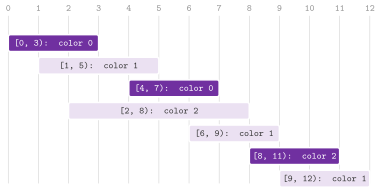
Algorithm 13.39. The greedy algorithms on intervals and on points of a line (Montresor 2025, §14.2 and exercises 14.6 and 14.7).
intervalColoring() (exercise 14.6) gives the fewest colors such that
intersecting intervals have different colors: it scans the \(2 n\) ends by
position, a right end before a left one equal to it, and a left end takes
a free color from a stack, a new one when the stack is empty, while a right
end gives its color back. towers() (exercise 14.7, the torri() of the
book) places the fewest towers such that each house, a point of the line,
is within \(d\) of one of them: a tower at \(k_0 + d\), \(k_0\) the first house,
serves the houses up to \(k_0 + 2 d\), and so on from the first house left
out.
Lemma 13.27. intervalColoring() uses
as many colors as the largest number of intervals over a point, and
towers() the fewest towers.
Proof. A new color is opened only when all the colors in use are held by intervals that contain the current point (the free ones having been given back by the right ends met before it, a right end equal to the point included), and then that many intervals and the new one share a point; any coloring needs as many colors as the intervals over a point (Montresor 2025, exercise 9.8). For the towers, some tower must serve the first house, and moving it to \(k_0 + d\) serves a superset of the houses that it served among those to its right. \(\square\)
The cover of a segment. minimumIntervalCover() of IntervalCover.h
finds the fewest closed intervals \([ a_i , b_i ]\) whose union contains the
segment \([ \mathit{lo} , \mathit{hi} ]\), e.g., the sprinklers at \(D_i\) of
radius \(R_i\), of intervals \([ D_i - R_i , D_i + R_i ]\), that water a lawn
\([ 0 , L ]\) (Kleinberg and Tardos 2005, §4.1).
With the part \([ \mathit{lo} , x ]\) already covered, the greedy takes,
among the intervals that start at \(x\) or before, the one that ends
farthest; if none ends beyond \(x\), the points just after \(x\) stay
uncovered and there is no cover (Algorithm 13.40).
On the intervals sorted by left end one scan finds the candidates of line
4, in \(O( n \log n )\) time for the sort, and the greedy is optimal
(Lemma 13.28). The
problem is the dual of the independent set of intervals, and the
one-dimensional case of the set cover, which in general is NP-hard and is
approximated within a factor \(\ln n\) by the greedy that takes the set with
the most new elements (Chvátal 1979;
see chapter 20).
Algorithm 13.40. The cover of a segment by the fewest intervals.
Lemma 13.28. If the intervals cover
\([ \mathit{lo} , \mathit{hi} ]\), minimumIntervalCover() returns a cover
by the fewest of them; otherwise it returns none.
Proof. Let \(g_1 , g_2 , \ldots\) be the intervals taken, and \(x_j\) the right end of \(g_j\) (\(x_0 = \mathit{lo}\)). Let \(o_1 , \ldots , o_q\) be a cover by the fewest intervals, sorted by right end; no \(o_j\) is contained in another, which could be dropped, and therefore the left ends are sorted too, and \(o_{j+1}\) starts at or before the end of \(o_j\), since otherwise the points between them would not be covered. We show \(x_j \ge b( o_j )\) by induction. The interval \(o_1\) contains \(\mathit{lo}\), and hence it is a candidate of line 4 at the first step. If \(x_j \ge b( o_j )\), then \(a( o_{j+1} ) \le b( o_j ) \le x_j\), and \(o_{j+1}\) is a candidate at the step \(j + 1\), unless it was taken before, in which case \(b( o_{j+1} ) \le x_j\). In both cases \(x_{j+1} \ge b( o_{j+1} )\). Also, the greedy does not stop at line 5 while \(x_j < \mathit{hi}\), since \(b( o_{j+1} ) > x_j\) there. Hence \(x_q \ge b( o_q ) \ge \mathit{hi}\), and the greedy takes at most \(q\) intervals. Conversely, if line 5 stops at \(x < \mathit{hi}\), every interval that starts at or before \(x\) ends at or before it, and the points between \(x\) and the least left end above \(x\) (or \(\mathit{hi}\)) are covered by no interval. \(\square\)
Scheduling. shortestJobFirst() orders \(n\) programs of durations
\(t_i\), run one after the other, in the order of least average time of
completion (Montresor 2025, exercise 14.5):
by increasing duration, since swapping two adjacent programs of which the
longer runs first does not increase the sum of the times of completion
(Lemma 13.29 below, with unit weights). With the weights \(w_i\)
of the programs (e.g., the probabilities of the files on a tape, which are
read, in fact, at the times of completion), the order of least weighted sum \(\sum_i
w_i C_i\) of the times of completion \(C_i\) is the rule of Smith
1956, by increasing \(t_i / w_i\)
(smithOrder(), Algorithm 13.41), compared
as \(t_a w_b < t_b w_a\), with no division, and a program of weight 0 thus goes
last. totalCompletion() and weightedCompletion() evaluate an order.
Algorithm 13.41. The shortest job first, and the rule of Smith.
Lemma 13.29. Swapping two adjacent programs \(a\) and \(b\), \(a\) first, leaves the times of completion of the others unchanged, and changes the weighted sum by
which is not negative if and only if \(t_a / w_a \le t_b / w_b\); hence the order by increasing \(t_i / w_i\) is optimal, and, for unit weights, the order by increasing \(t_i\).
Proof. Let \(s\) be the time at which the pair starts. Before the swap the pair contributes \(w_a ( s + t_a ) + w_b ( s + t_a + t_b )\), after it \(w_b ( s + t_b ) + w_a ( s + t_a + t_b )\), and the difference is (13.19). An order with an adjacent pair against the rule is therefore not worse after the swap, and a finite sequence of such swaps (those of the bubble sort) turns any order into the order of the rule. \(\square\)
With precedence constraints among the programs the problem is NP-hard in general, and it is solved by the merging of chains of Lawler 1978 on the series-parallel orders.
Matching points on a line. lineAssignment() of SequenceQueries.h
(exercise 14.8) finds the least sum of \(\lvert h_i - l_{\pi( i )} \rvert\)
over the matchings \(\pi\) of two sets of \(n\) points on a line, by sorting
both and matching them in order (Algorithm 13.42),
in \(O( n \log n )\) time against the \(O( n^3 )\) of the Hungarian method on
general costs (Kuhn 1955). For \(h_1 \le
h_2\) and \(l_1 \le l_2\) one has
and the same holds for any convex function in place of the absolute value, as the next lemma shows.
Lemma 13.30. Let \(f\) be convex. For
\(h_1 \le h_2\) and \(l_1 \le l_2\), \(f( h_1 - l_1 ) + f( h_2 - l_2 ) \le
f( h_1 - l_2 ) + f( h_2 - l_1 )\); hence matching the two sets in sorted
order minimizes \(\sum_i f( h_i - l_{\pi( i )} )\), and lineAssignment()
is optimal.
Proof. Let \(\alpha = h_1 - l_1\), \(\delta = h_2 - l_2\), \(\beta = h_1 - l_2\) and \(\gamma = h_2 - l_1\). Then \(\beta \le \alpha \le \gamma\), \(\beta \le \delta \le \gamma\) and \(\alpha + \delta = \beta + \gamma\); hence \(\alpha\) and \(\delta\) are the convex combinations \(\lambda \beta + ( 1 - \lambda ) \gamma\) and \(( 1 - \lambda ) \beta + \lambda \gamma\) for some \(\lambda \in [ 0 , 1 ]\) (any, if \(\beta = \gamma\)), and adding the two inequalities of convexity gives the claim. Thus a matching with a crossing, i.e., \(h_i \le h_j\) and \(l_{\pi( i )} > l_{\pi( j )}\), does not get worse when the two partners are exchanged, and each exchange lowers the number of the crossings, which is finite, until the matching is the sorted one. \(\square\)
With \(f = \lvert \cdot \rvert\) this is (13.20); for any convex \(f\) it is
the optimal transport on the line. Its sum is computed in a type W given
by the caller, wider than the points if needed.
Algorithm 13.42. The cheapest matching of two sets of points on a line.
Where the greedy choice fails. For the change with the fewest coins
(CoinChange.h, the introduction of Montresor 2025,
chapter 14), greedyChange() takes
the largest coin that fits as many times as it fits
(Algorithm 13.43). It is optimal for the
coins of 50, 10, 5 and 1 cents, but not for coins of 11, 5 and 1, where it
pays 15 with five coins (\(11 + 1 + 1 + 1 + 1\)) instead of three of 5; also,
it may fail to pay an amount that other coins pay, e.g., 6 with coins of 4
and 3. Then the dynamic programming optimalChange() of
§13.8 is needed, whose entries on the second
system we show in Table 13.6. In the same way, the sum of four squares of minimumSquares() is
not found by taking the largest square first, \(18 = 9 + 9\) instead of \(16 +
1 + 1\), and no order of the objects is optimal for the 0-1 knapsack.
Algorithm 13.43. The change by the greedy choice.
Table 13.6. The fewest coins \(N[ x ]\) of
optimalChange() for the coins 11, 5 and 1 and the amounts \(x\) up to 15;
the greedy choice pays 15 with five coins.
| \(x\) | 0 | 1 | 2 | 3 | 4 | 5 | 6 | 7 |
|---|---|---|---|---|---|---|---|---|
| \(N[ x ]\) | 0 | 1 | 2 | 3 | 4 | 1 | 2 | 3 |
| \(x\) | 8 | 9 | 10 | 11 | 12 | 13 | 14 | 15 |
| \(N[ x ]\) | 4 | 5 | 2 | 1 | 2 | 3 | 4 | 3 |
A system of coins for which the greedy choice is optimal for every amount is called canonical; the usual systems of the currencies are, and whether a system is canonical can be decided in polynomial time; we do not dwell further on it here, since the library does not implement the test.
The greedy algorithms of the section are declared as follows:
// declarations of <ADS/optimization/FractionalKnapsack.h>
//                  <ADS/optimization/Intervals.h>
//                  <ADS/optimization/IntervalCover.h>
//                  <ADS/optimization/ShortestJobFirst.h>
//                  <ADS/optimization/CoinChange.h>
//                  <ADS/algorithm/SequenceQueries.h>
std::vector< double > fractionalKnapsack( const std::vector< double > & p ,
                                          const std::vector< double > & v ,
                                          double C );
std::vector< std::size_t >
independentSet( const std::vector< std::pair< long , long > > & I );
std::vector< int >
intervalColoring( const std::vector< std::pair< long , long > > & I );
std::vector< double > towers( std::vector< double > k , double d );
template< class T >
std::optional< std::vector< std::size_t > >
minimumIntervalCover( const std::vector< std::pair< T , T > > & I , T lo ,
                      T hi );
template< class T >
std::vector< std::size_t > shortestJobFirst( const std::vector< T > & t );
template< class T , class W >
std::vector< std::size_t > smithOrder( const std::vector< T > & t ,
                                       const std::vector< W > & w );
template< class T >
T totalCompletion( const std::vector< T > & t ,
                   const std::vector< std::size_t > & A );
template< class T , class W >
auto weightedCompletion( const std::vector< T > & t ,
                         const std::vector< W > & w ,
                         const std::vector< std::size_t > & A );
template< class T , class W = T >
 requires std::is_arithmetic_v< T >
W lineAssignment( std::vector< T > H , std::vector< T > L );
std::optional< std::vector< long > > greedyChange( std::vector< long > coins ,
                                                   long c );
13.12 Monte Carlo algorithms¶
An algorithm of Monte Carlo always ends within its bound, and it may
answer wrongly with a probability bounded over its random choices, not
over the inputs (Montresor 2025, chapter 17).
In MonteCarlo.h, the three algorithms take the generator of random
numbers as a parameter, and either have a one-sided error, which \(K\)
independent runs lower to its \(K\)-th power, or an error that \(K\) samples
lower exponentially (Table 13.7).
Lemma 13.31 (Schwartz and Zippel). A nonzero polynomial of total degree \(d\) in \(n\) variables vanishes at a point drawn uniformly from \(S^n\) with probability at most \(d / \lvert S \rvert\).
Proof. For one variable, a nonzero polynomial of degree \(d\) has at most \(d\) roots. For \(n\) variables, write the polynomial as one in \(x_1\) of degree \(e\), whose leading coefficient is a nonzero polynomial of total degree at most \(d - e\) in the other variables: by induction, the coefficient vanishes with probability at most \(( d - e ) / \lvert S \rvert\), and if it does not, the polynomial in \(x_1\), of degree \(e\) once the other variables are fixed, vanishes with probability at most \(e / \lvert S \rvert\) over \(x_1\); the two bounds add up to \(d / \lvert S \rvert\). \(\square\)
Hence zeroPolynomial(), which evaluates a polynomial \(p\) of total degree
\(d\), given as a function of its \(n\) variables, at \(K\) points drawn from
\(\{ 1 , \ldots , 2 \max( d , 1 ) \}^n\), errs with probability at most \(1 /
2\) per run, and only when it answers that \(p\) is zero; a point where \(p \ne
0\) proves that it is not (Schwartz 1980;
Zippel 1979). Its points are of the
type long, and its precondition is thus that \(2 d\) is a long, i.e.,
\(d \le \mathrm{LONG\_MAX} / 2\), beyond which the set \(S\) could not be
drawn. In the same way, the algorithm of
Freivalds 1977 (freivalds(),
exercise 17.4) applies the same argument to the matrix \(M = A B - C\) of
three \(n \times n\) matrices: it compares \(A ( B x )\) with \(C x\) for a random
vector \(x\) of \(\pm 1\) (Algorithm 13.44).
Algorithm 13.44. The test of a polynomial identity, the algorithm of Freivalds, and the estimate of the satisfying assignments.
Lemma 13.32. If \(A B \ne C\), a run of
freivalds() answers that they are equal with probability at most \(1 /
2\); each run costs \(O( n^2 )\) time.
Proof. Some row \(m\) of \(M = A B - C\) is not zero, say \(m_j \ne 0\). For each choice of the other signs of \(x\), the two values \(m \cdot x\) given by \(x_j = 1\) and \(x_j = -1\) differ by \(2 m_j \ne 0\), and at most one of them is 0; hence \(M x = 0\) with probability at most \(1 / 2\). A run makes three products of a matrix by a vector. \(\square\)
Hence, the test costs \(O( K n^2 )\), against the product of two matrices.
Last, halfSatisfiable() (exercise 17.5) decides whether a boolean
formula of \(n\) variables is true on more than half of the assignments, by
the fraction of the true ones among \(K\) random assignments. If the true
fraction is \(1 / 2 + \epsilon\), the bound of Hoeffding
1963 gives
\(Y\) being the number of the true samples, and symmetrically for \(1 / 2 - \epsilon\); the error is two-sided, and \(K\) must grow as \(1 / \epsilon^2\), which may be "large" when the fraction is close to \(1 / 2\).
Table 13.7. The algorithms of Monte Carlo
of MonteCarlo.h and their errors after \(K\) runs or samples.
| Function | Error | Probability of error | Time |
|---|---|---|---|
zeroPolynomial() |
one-sided, on "zero" | \(2^{-K}\) | \(K\) evaluations of \(p\) |
freivalds() |
one-sided, on "equal" | \(2^{-K}\) | \(O( K n^2 )\) |
halfSatisfiable() |
two-sided | \(e^{-2 K \epsilon^2}\) | \(K\) evaluations of the formula |
The three algorithms take the generator rng of the caller and the
number \(K\) of the runs or of the samples:
// declarations of <ADS/algorithm/MonteCarlo.h>
template< class F , class R >
bool zeroPolynomial( F && p , std::size_t n , long d , int K , R & rng );
template< class T , class R >
bool freivalds( const std::vector< std::vector< T > > & A ,
                const std::vector< std::vector< T > > & B ,
                const std::vector< std::vector< T > > & C , int K , R & rng );
template< class F , class R >
bool halfSatisfiable( F && f , std::size_t n , int K , R & rng );
13.13 Discussion and references¶
We took the master theorem, its version with the logarithms and the recurrences that decrease by a constant from Montresor 2025, §2.9; the theorem of Akra and Bazzi 1998, with the perturbations of Leighton 1996, covers the parts of different sizes, and Cormen et al. 2022 discusses both. Amortized analysis goes back to Tarjan 1985, and the elimination of the recursion by the systematic rules is in Montresor 2025, §4.4. For the segments of largest sum, and the progression from the cubic algorithm to the linear scan, we followed Bentley 1984 and Ferragina 2023, chapter 2, with the variants for the bounded length of Lin, Jiang and Chao 2002 and for the density of Goldwasser, Kao and Lu 2005 and Chung and Lu 2005. Our presentation of the dynamic programming and of the greedy algorithms follows Montresor 2025, chapters 13 and 14 and its collections of exercises, with Kleinberg and Tardos 2005, chapters 4 and 6 for the exchange arguments and the weighted intervals, and Martello and Toth 1990 for the knapsack and its variants. As for the optimal search trees, the speedup is due to Knuth 1971, and its general form, the quadrangle inequality, to Yao 1980; the alphabetic trees are those of Hu and Tucker 1971 and Garsia and Wachs 1977. The longest increasing subsequence in \(O( n \log n )\) is due to Fredman 1975, its weighted form to Jacobson and Vo 1992. The rule of Smith 1956 is one of the first results of scheduling theory, and, finally, the lemma of Schwartz 1980 and Zippel 1979, the test of Freivalds 1977 and the bound of Hoeffding 1963 are the standard tools of the randomized algorithms.
13.14 Exercises¶
Each exercise names the test of the library that solves it (run it with
ctest -R <name>).
- Solve the recurrences of divide et impera by the master theorem,
including the case \(k = -1\), and those that decrease the size by a
constant; check that \(\log_{10} 1000\) does not move a recurrence to
another case. Test:
ch02.sec2.9.recurrences. - Find the exponent of Akra and Bazzi of \(T( n ) = T( n / 5 ) + T( 7 n /
10 ) + n\) by bisection, and conclude that the selection is linear.
Test:
lib_optimization.akra-bazzi. - Show that \(n\) increments of a binary counter change fewer than \(2 n\)
bits, both by aggregation and by a potential. Test:
ch04.sec4.2.1.counter. - Make the towers of Hanoi iterative, once by eliminating the tail call
and once by the systematic rules, and check that the three procedures
make the same \(2^n - 1\) moves. Test:
ch04.sec4.4.hanoi. - Instantiate each general scheme: the linear search, the sort and the
0-1 knapsack by the enumeration (the knapsack checked against
knapsack()), the \(n\) queens by backtracking, the minimum and the maximum by divide et impera, the change by the greedy scheme, and the maximal elements of a list for three partial orders. Test:beyond.paradigms. - Find a segment of largest sum by the four algorithms of the cubic,
quadratic and linear time, and check that they agree on random arrays.
Test:
pearls_io.ch2.max-sum-random. - Find a segment of largest sum with the length in \([ L , U ]\) in \(O( n
)\) time by a deque of the starts. Test:
pearls_io.ch2.length-constrained. - Find the longest segment of sum at least \(t\), and of average at least
\(p / q\), in \(O( n )\) time by the chain of the leftmost minima. Test:
pearls_io.ch2.longest-at-least. - Find the segment of largest density of C and G of a DNA sequence among
those of length at least \(L\). Test:
pearls_io.ch2.density. - Find a longest increasing subsequence in \(O( n^2 )\) and its length in
\(O( n \log n )\) (Montresor 2025, exercise
13.6). Test:
ch13.ex13.6. - Count the smaller items on the right of each item of a sequence in \(O(
n \log n )\) time, and find the longest run with at most \(k\) values,
the largest gap of a set of intervals and the cheapest matching of two
sets of points on a line. Test:
lib_search.sequence-queries. - Solve the 0-1 knapsack bottom up and by memoization, and count the
subproblems that the memoization solves. Test:
ch13.sec13.6.knapsack. - Solve the unbounded knapsack and the cut of a rod, reading back the
copies and the pieces. Tests:
lib_optimization.unbounded-knapsack,lib_optimization.rod-cutting. - Count the ways of paying an amount with coins in unlimited supply and
the subsets of a given sum, and explain why the two loops run in
opposite directions. Test:
lib_optimization.coin-change-ways. - Find the fewest squares that sum to \(n\) in \(O( \sqrt n \log n )\) time. Test:
lib_optimization.minimum-squares. - Solve the independent set of weighted intervals in \(O( n \log n )\)
time (Montresor 2025, §13.2).
Test:
ch13.sec13.2.intervals. - Find the largest gain of at most \(k\), and of exactly \(k\),
transactions on a stock in \(O( n k )\) time. Test:
lib_optimization.stock-trading. - Find the largest sum of items no two of them adjacent, and the
cheapest painting of a row of houses in \(O( n k )\) time. Test:
lib_optimization.house-problems. - Find the largest divisible subset, the heaviest increasing
subsequence, the longest chain in a partial order and the longest
segment with no value repeated. Test:
lib_optimization.sequence-problems. - Compute the optimal binary search tree in \(O( n^2 )\) time by the bound
of Knuth on the roots. Test:
lib_optimization.optimal-search-tree. - Solve the game of the coins in a line in \(\Theta( n^2 )\) time and
\(\Theta( n )\) space. Test:
lib_optimization.coins-in-a-line. - Split a sequence into \(k\) parts of least largest sum, by dynamic
programming and by a binary search on the answer. Test:
lib_optimization.linear-partition. - Find the largest square of ones of a matrix and count the lattice
paths through a grid with blocked cells. Test:
lib_optimization.grid-paths. - Solve the fractional knapsack by the greedy choice, and show that no
greedy order is optimal for the 0-1 knapsack. Tests:
ch14.sec14.1.real-knapsack,ch14.ex14.1. - Show that the greedy change is optimal for the coins of 50, 10, 5 and
1, but not for those of 11, 5 and 1. Test:
ch14.sec14.change. - Color a set of intervals with the fewest colors, and place the fewest
towers that serve a set of houses. Tests:
ch14.ex14.6,ch14.ex14.7. - Cover a segment with the fewest intervals. Test:
lib_optimization.interval-cover. - Order \(n\) programs to minimize the weighted sum of the times of
completion by the rule of Smith. Test:
lib_optimization.smith-rule. - Decide whether \(A B = C\) by the algorithm of Freivalds in \(O( K n^2 )\)
time, and bound its error. Test:
ch17.ex17.4. - Decide whether a polynomial is identically zero, and whether a formula
is true on more than half of its assignments. Tests:
ch17.sec17.monte-carlo,ch17.ex17.5.