21. Compression¶
[Source: include/ADS/compression/Entropy.h, CanonicalHuffman.h,
HuffmanCoder.h, PackedBits.h, ArithmeticCoding.h, Rans.h,
Tans.h, PPM.h, IntegerCodes.h, BinaryPacking.h, StreamVByte.h,
DirectAccessCodes.h, LempelZiv.h, LZ77Linear.h, BurrowsWheeler.h,
FMIndex.h, HuffmanFMIndex.h, RIndex.h, MoveRIndex.h]
We are concerned in this chapter with the lossless compression of a text,
i.e., with an encoder that turns a string of symbols into a shorter string
of bits and a decoder that gives the string back, and with the indexes that
search a text kept in compressed form. The headers of ADS/compression
follow chapters 11 to 14 of Ferragina 2023
(Integer Coding, Statistical Coding, Dictionary-Based Compressors and
Block-Sorting Compression), which the book of Montresor meets only in the
code of Huffman of its section 14.4. Beside each algorithm of the book they
give the engineered form that the fast compressors of today use. We first
fix the measure against which a compressor is judged, the empirical entropy
(§21.1). Then come the statistical codes,
which give each symbol a number of bits that depends on its probability:
the code of Huffman, as the book presents it and as the coders by tables
decode it (§21.2 and
§21.3), the arithmetic code
(§21.4), the asymmetric numeral systems
(§21.5) and the prediction by partial matching
(§21.6). We treat the codes of the integers, which assume a distribution instead of measuring one, in §21.7, and their engineered forms in
§21.8. Two families of compressors need no
model at all: those of Lempel and Ziv replace a string with a reference to
an earlier occurrence of it (§21.9), and the
transform of Burrows and Wheeler sorts the contexts of the symbols, after
which the symbols are easy to code (§21.10).
The transform is also an index of the text, which
§21.11 builds in four forms of decreasing
space. In the sets of §1.9,
ArithmeticCoding.h, BurrowsWheeler.h, CanonicalHuffman.h,
Entropy.h, FMIndex.h, IntegerCodes.h, LempelZiv.h and PPM.h are
base and the other headers of this chapter are advanced, while
PackedBits.h is in the core that the two sets include.
21.1 Entropy¶
A text \(s = s[ 0 ] s[ 1 ] \cdots s[ n - 1 ]\) is a string of \(n\) symbols of an ordered alphabet \(\Sigma\) of \(\sigma\) symbols (usually the bytes); we write \(s[ i .. j ]\) for the substring from \(i\) to \(j\), \(s[ i .. ]\) for the suffix from \(i\), and \(n_c\) for the occurrences of the symbol \(c\) in \(s\). We call code a map of each symbol \(c\) to a binary codeword of length \(\ell( c )\), and of a text to the concatenation of the codewords of its symbols; we say that it is prefix-free when no codeword is a prefix of another one; then the concatenation is decoded from left to right with no separator, since a codeword is recognized when its last bit is read. Table 21.1 collects the notation that the headers of the area share.
Table 21.1. The notation of the chapter.
| Symbol | Meaning |
|---|---|
| \(n_c\), \(P[ c ]\) | the occurrences of \(c\) in \(s\), and its probability (\(n_c / n\) for the empirical one) |
| \(H_0\), \(H_k\) | the entropy of order 0 and of order \(k\), in bits per symbol, (21.1) and (21.2) |
| \(\ell( c )\), \(\bar\ell\) | the length of the codeword of \(c\), and the average \(\sum_c P[ c ] \ell( c )\) |
| \(B( x )\) | the binary code of the integer \(x \ge 1\), of \(1 + \lfloor \log_2 x \rfloor\) bits |
| \(\mathit{SA}\) | the suffix array of \(s \$\), with \(\$\) a sentinel smaller than all the symbols |
| \(F\), \(L\) | the first and the last column of the sorted rotations of \(s \$\) |
| \(C[ c ]\) | the symbols of \(s \$\) smaller than \(c\) |
| \(\mathrm{rank}_c( L , i )\) | the occurrences of \(c\) in \(L[ 0 .. i - 1 ]\) |
| \(r\), \(z\) | the runs of equal symbols of \(L\), and the phrases of a parse of Lempel and Ziv |
| \(p\), \(\mathit{occ}\) | the length of a pattern \(P\), and the number of its occurrences in \(s\) |
The entropy of order 0 of a distribution \(P\) on \(\Sigma\), and the empirical entropy of \(s\), which takes \(P[ c ] = n_c / n\), are
where the term of a symbol of probability 0 is 0 (Shannon 1948). One has \(0 \le H_0 \le \log_2 \sigma\) (cf. (21.1)), with 0 when one symbol has all the probability and \(\log_2 \sigma\) when the symbols are equally likely. As Lemma 21.1 shows, no code of the symbols one by one takes fewer than \(n H_0\) bits on average. A code that looks at the context of a symbol may do much better on the texts of a language, where a symbol is often (but not always) all but fixed by the few symbols before it. With \(w_s\) the string of the symbols that follow the occurrences of \(w\) in \(s\), in their order, the entropy of order \(k\) of \(s\) is
the average entropy of the symbols in their contexts of \(k\) symbols
(Manzini 2001). One has
\(H_{k+1} \le H_k \le H_0\), since conditioning on a longer context does not
increase the entropy, and \(n H_k\) is the measure of the compressors of
order \(k\). In Entropy.h, three functions entropy() compute (21.1)
on a map of frequencies and on a string, and (21.2) on a string
(Algorithm 21.1). They take \(O( n \log n )\)
time, with the counts in ordered maps, and their contract checks that
\(H_k \le H_0\) on the result, up to the rounding.
Algorithm 21.1. The empirical entropies of order 0 and of order \(k\).
We remark that (21.2) divides by \(n\) while only the \(n - k\) symbols with a full context of \(k\) symbols are counted. Indeed, the first \(k\) symbols are left out of the sum, as in the definition of Manzini, and their contribution vanishes as \(n\) grows.
21.2 Prefix-free codes and the code of Huffman¶
We first show that the lengths of a prefix-free code cannot be all "small", and the bound on them is also a bound on the average length of the code.
Lemma 21.1 (Kraft and Shannon). The lengths of a prefix-free code satisfy
any lengths that satisfy (21.3) are those of a prefix-free code, and the average length of a prefix-free code is at least \(H_0\).
Proof. A codeword of length \(\ell( c )\) is a node at the depth \(\ell( c )\) of the complete binary tree of depth \(\ell_{\max} = \max_c \ell( c )\). Since no codeword is an ancestor of another one, the \(2^{\ell_{\max} - \ell( c )}\) leaves below the codewords are disjoint, which is (21.3) multiplied by \(2^{\ell_{\max}}\). Conversely, the canonical code below (Lemma 21.2) gives prefix-free codewords of any lengths that satisfy (21.3). Finally, by the concavity of the logarithm (the inequality of Jensen) and by (21.3),
Hence one can see that the lengths \(\ell( c ) = \log_2( 1 / P[ c ] )\) would reach \(H_0\) if
they were integers, and the question is how close to \(H_0\) the integer
lengths can come. This is answered by the code of Huffman 1952. It merges the two least probable symbols into one of their
total probability, \(\sigma - 1\) times, and the codewords of the two are
those of the merged symbol followed by 0 and by 1. In ADS we make the merges by huffman() of ADS/string/Huffman.h, with a heap, in
\(O( \sigma \log \sigma )\) time, and huffmanLengths() of
CanonicalHuffman.h reads the lengths off its codewords.
Theorem 21.1 (Huffman). The code of Huffman has the least average length among the prefix-free codes of the symbols, and
Proof. We show by induction on \(\sigma\) that the merges give an optimal code; for \(\sigma \le 2\) the codewords have at most 1 bit. Let \(x\) and \(y\) be the two least probable symbols. The tree of an optimal code is full (a node with one child could be replaced by the child, shortening the codewords below it), and hence its deepest level holds two sibling leaves; exchanging their symbols with \(x\) and \(y\) does not increase the average, since \(x\) and \(y\) are the least probable, and therefore some optimal code \(T\) has \(x\) and \(y\) as sibling leaves. Replacing the two leaves with a leaf of a new symbol \(z\) of probability \(P[ x ] + P[ y ]\) gives a code \(T'\) of \(\sigma - 1\) symbols with \(\bar\ell( T ) = \bar\ell( T' ) + P[ x ] + P[ y ]\). The code \(H\) of the merges is the code \(H'\) of the merges on the \(\sigma - 1\) symbols with \(z\) in place of \(x\) and \(y\), whose leaf is split into the two, and \(\bar\ell( H ) = \bar\ell( H' ) + P[ x ] + P[ y ]\) in the same way. By induction \(\bar\ell( H' ) \le \bar\ell( T' )\), and hence \(\bar\ell( H ) \le \bar\ell( T )\). As for (21.4), its lower bound is Lemma 21.1, and its upper bound holds since the lengths \(\lceil \log_2( 1 / P[ c ] ) \rceil\) satisfy (21.3) and have an average below \(H_0 + 1\), and the optimum is no longer than they are. \(\square\)
We remark that only the lengths of a code matter for its size. We call canonical a code that gives the symbols of each length consecutive codewords, in the order of the symbols, and therefore neither the encoder nor the decoder needs the tree (Schwartz and Kallick 1964). With \(\mathit{num}[ l ]\) the symbols of length \(l\) and \(\ell_{\max}\) the longest length, the first codeword of each length is
i.e., the parent of the first node of the level \(l + 1\) that is not used. Then the symbols of length \(l\) get the codewords \(\mathit{fc}[ l ]\), \(\mathit{fc}[ l ] + 1\), and so on, on \(l\) bits (Algorithm 21.2), and hence the tree is skewed to the left, the longest codewords being all zeros at the start (Figure 21.1). Chapter 12 of Ferragina 2023 divides in (21.5) without rounding up. This is the same on the "complete" codes that the merges of Huffman give (the sum is even there), while the ceiling also keeps the decoder right on a code that is not complete, e.g., one cut by a limit on the lengths.
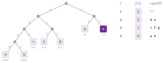
Algorithm 21.2. The canonical code of given lengths, and the decoding of a codeword (Ferragina 2023, chapter 12, Statistical Coding).
Lemma 21.2. If the lengths satisfy (21.3), the codewords of (21.5) fit in their lengths, the code is prefix-free, and the decoding of Algorithm 21.2 returns the symbol whose codeword is next in the input.
Proof. Let \(a_l = \mathit{fc}[ l ] + \mathit{num}[ l ]\), the value past the last codeword of length \(l\), and \(K_l = \sum_{l' \ge l} \mathit{num}[ l' ] \, 2^{-l'}\). By induction from \(l = \ell_{\max}\) down, \(a_l \le \lceil 2^l K_l \rceil\): it holds with equality at \(\ell_{\max}\), and \(\mathit{fc}[ l ] = \lceil a_{l+1} / 2 \rceil \le \lceil 2^l K_{l+1} \rceil\) gives \(a_l \le \lceil 2^l K_{l+1} \rceil + \mathit{num}[ l ] = \lceil 2^l K_l \rceil\). Since \(K_l \le 1\) by (21.3), \(a_l \le 2^l\), i.e., the codewords of length \(l\) fit in \(l\) bits. Next, the first \(l\) bits of a codeword \(v\) of length \(l + 1\) are \(\lfloor v / 2 \rfloor \le \lfloor ( a_{l+1} - 1 ) / 2 \rfloor < \lceil a_{l+1} / 2 \rceil = \mathit{fc}[ l ]\). By induction on the length, the first \(l\) bits of a longer codeword are below \(\mathit{fc}[ l ]\) too, since its first \(l + 1\) bits are below \(\mathit{fc}[ l + 1 ] \le 2 \, \mathit{fc}[ l ]\). Hence no codeword of length \(l\), which is at least \(\mathit{fc}[ l ]\), is a prefix of a longer one. Finally, the decoder reads one bit at a time and stops at the first \(l\) at which the value \(v\) of the bits read reaches \(\mathit{fc}[ l ]\), i.e., at the end of the codeword, whose symbol is the \(( v - \mathit{fc}[ l ] )\)-th of length \(l\). \(\square\)
Hence the preamble of a canonical code is the lengths alone (cf. (21.5)). Also, we decode a codeword of \(l\) bits by \(l\) steps on two arrays that fit in the cache, instead of \(l\) steps along the pointers of a tree, each a possible miss. The implementation follows the pseudocode, with \(\mathit{fc}[ 1 .. \ell_{\max} ]\) and the symbols by length in vectors.
Encoding a symbol is a lookup of its codeword and its length in
\(O( 1 )\) time (Algorithm 21.3), and the
construction takes \(O( \sigma \log \sigma )\) time. The class (whose
symbols are of the type symbol_type) is built from the lengths or, by
fromFrequencies(), from the frequencies through huffmanLengths();
maxLength() gives the longest length and firstCode( l ) the value
\(\mathit{fc}[ l ]\) of the first codeword of length \(l\). We write and read the bits by PackedBitWriter and PackedBitReader of PackedBits.h, which pack them in bytes with the first bit in the most significant bit of the
first byte, and whose position() counts the bits read (past the end
too). Hence the value of the bits read so far is the integer whose
binary digits they are, which is the order in which the canonical decoder
and the arithmetic decoder of §21.4 read
their input; a reader also gives zeros past the end of its bytes, as the
arithmetic decoder expects. (The two classes only move bits, and we therefore give them no pseudocode.)
Algorithm 21.3. The encoding of a text by the canonical code, and the lengths of a code of Huffman of no length above \(L\) by the iterative scaling of the frequencies.
The codewords of Huffman can be rather long. Frequencies that grow as the numbers
of Fibonacci give a codeword of 33 bits after about \(10^7\) symbols
(Ferragina 2023, chapter 12), while a "fast" decoder typically wants the codewords to fit in a word, or in the index of a
table. The function limitedLengths() bounds them to a given \(L\) by halving the
frequencies, rounding up, until the code of Huffman of the halved ones has
no length above \(L\).
Lemma 21.3. If \(2^L \ge \sigma\), the loop
of limitedLengths() ends after at most
\(\lceil \log_2 f_{\max} \rceil + 1\) codes of Huffman, \(f_{\max}\) being the
largest frequency.
Proof. Halving with rounding up maps 1 to 1 and any frequency \(f \ge 2\) to \(\lceil f / 2 \rceil < f\), and after \(\lceil \log_2 f_{\max} \rceil\) halvings all the frequencies are 1, since \(f \le 2^k\) gives \(\lceil f / 2 \rceil \le 2^{k-1}\). On \(\sigma \ge 2\) equal frequencies, the tree of the code of Huffman is full and optimal (Theorem 21.1), and its leaves lie on two consecutive levels: if a leaf were at a depth \(d \le D - 2\), with \(D\) the largest depth, moving two sibling leaves of depth \(D\) below it would turn their parent into a leaf and change the sum of the depths by \(-2 D + ( D - 1 ) - d + 2 ( d + 1 ) = d + 1 - D < 0\), against the optimality. With the leaves on the levels \(D - 1\) and \(D\), each of the \(2^{D-1}\) nodes of the level \(D - 1\) is a leaf or has two children, and at least one has children; hence \(\sigma \ge 2^{D-1} + 1\), i.e., \(D \le \lceil \log_2 \sigma \rceil \le L\), and the loop ends there at the latest. \(\square\)
Halving is simple but (possibly) not optimal: when it comes to the end it gives a code of fixed length, whereas the package-merge of Larmore and Hirschberg 1990 finds the optimal code of lengths at most \(L\) in \(O( \sigma L )\) time (see §21.3).
21.3 The code of Huffman with tables¶
The functions huffmanCompress() and huffmanDecompress() of HuffmanCoder.h code a
string of bytes as the fast coders do, with the code of Huffman of the
bytes and four choices that the canonical code of
§21.2 does not make. First, the lengths are
the optimal ones of at most 11 bits, found by the package-merge of
Larmore and Hirschberg 1990
(Algorithm 21.4), and the decoding table
therefore stays in the cache of the first level. This limit usually costs a fraction of a percent on a text of bytes, since the optimum under it is
found exactly. Second, the code is canonical, and its preamble is the
lengths of the 256 bytes in 4 bits each. Third, the codewords are written
from the least significant bit of a word of 64 bits, each turned around to
keep the code prefix-free in the order of reading, and four of them are
joined by shifts and stored at once. Fourth, the input is cut in four
quarters, each coded into a separate stream. Since the four streams are decoded together, the four chains of dependences of the decoder (a lookup gives
the length of a codeword, which gives the place of the next lookup) overlap
in the pipeline of the processor; this is the interleaving of Zstandard
(Collet and Kucherawy 2021).
Algorithm 21.4. The optimal lengths of at most \(L\) bits by package-merge (Larmore and Hirschberg 1990), and the compression of a string of bytes.
Our decoder peeks at the next \(W\) bits of a stream, and hopefully finds more than one codeword there. In a table of \(2^W\) entries of 32 bits it finds the symbols whose codewords fit whole in them, up to 3 in the low 24 bits of the entry, followed by the number of their bits in 4 bits and by the number of the symbols in 2 (Figure 21.2). A lookup is two shifts and a mask, and therefore it has no branch, and it may decode about \(\min( 3 , \lfloor W / \bar\ell \rfloor )\) symbols for an average length \(\bar\ell\); these are the decoders by tables of Moffat and Turpin 1997. Its window is \(W = 12\) bits from \(2^{18}\) bytes on, a table of 16 KB that gives more symbols a lookup, and \(W = 11\) below, where half the table is somewhat quicker to build. Since a codeword has at most 11 bits, it fits whole in any window, and each lookup on a valid stream decodes at least one symbol.
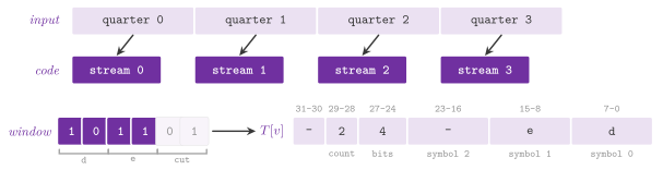
Algorithm 21.5. The decompression by the tables of up to 3 symbols, on four streams.
Four lookups of at most 12 bits fit in the bits of a word after a refill, which leaves at least 57 bits to read, and the loop of the decoder therefore loads each word once each four lookups. Note that each lookup stores the 4 bytes of its entry, of which the next lookup overwrites those past its symbols.
This loop runs while each stream has room for 12 more symbols, and the rest
is decoded one symbol at a time with the table of the single symbols. A
string of one distinct byte is written as that byte and its count, since
the code of Huffman of one symbol has no bit. Also, the loads and the stores of little-endian words at any address, and the histogram of the bytes on
eight tables of counts (one for each byte of a word, so that a run of equal
bytes does not wait for the store of the count before), are in the
internal header impl/Unaligned.h, shared with the coders of
§21.5; we do not describe it further. In size, we have the code of Huffman of the bytes, within one
bit per byte of \(H_0\) by (21.4). Its speed comes from the table and from
the streams, as Table 21.2 summarizes for the
statistical coders of the chapter.
Table 21.2. The statistical coders of the area on a text of \(n\) symbols, and their costs.
| Coder | Bits | Time per symbol | Model |
|---|---|---|---|
CanonicalHuffman |
\(n \bar\ell_H < n ( H_0 + 1 )\) | \(O( \ell( c ) )\) to decode, a bit at a time | static, any alphabet, the lengths as preamble |
huffmanCompress() |
as above, lengths at most 11 | up to 3 symbols per lookup to decode | static, bytes, four streams |
arithmeticEncode() |
\(\le 2 + n H_0\) (exact), about \(10^{-4} n\) more on 32 bits | \(O( \log \sigma )\) adaptive (a tree of Fenwick) | static or adaptive |
ransCompress(), tansCompress() |
\(n H_0\) plus a fraction of a percent | \(O( 1 )\), a multiplication or a lookup | static, bytes |
ppmEncode() |
approaches \(n H_K\) plus the escapes | \(O( K ( K + \sigma_K ) \log n )\) | contexts of up to \(K\) symbols |
21.4 The arithmetic code¶
As we have seen, a code of the symbols one by one may lose up to one bit per symbol against \(H_0\) by (21.4), which is "much" on a skewed distribution: a symbol of probability 0.99 carries about 0.015 bits of information, and it costs 1 bit anyway. Instead, the arithmetic code codes the text as one number. With the cumulative probabilities \(f_c = \sum_{c' < c} P[ c' ]\), the symbols narrow an interval \([ l , l + s )\) of \([ 0 , 1 )\) in turn, each to the part of its probability,
and the code is a short binary fraction inside the last interval (Figure 21.3).
Theorem 21.2 (the arithmetic code). With \(s_n = \prod_i P[ s[ i ] ]\) the size of the last interval \([ l_n , l_n + s_n )\), the first \(d = \lceil \log_2( 2 / s_n ) \rceil\) bits of \(l_n + s_n / 2\) are a prefix-free code of \(s\) among the texts of \(n\) symbols, and with the empirical probabilities
Proof. Truncating \(x = l_n + s_n / 2\) to \(d\) bits loses less than \(2^{-d} \le s_n / 2\). Hence the fraction \(x'\) written, and each fraction that begins with its bits, lie in \([ x' , x' + 2^{-d} ) \subseteq [ l_n , l_n + s_n )\). Moreover, the intervals of two texts of \(n\) symbols are disjoint, since (21.6) splits each interval into disjoint parts, and therefore no code is a prefix of another one. Finally, the sum in (21.7) is \(\sum_c n_c \log_2( n / n_c ) = n H_0\), and \(d < \log_2( 2 / s_n ) + 1 = 2 + \log_2( 1 / s_n )\). \(\square\)
We see that the arithmetic code is within 2 bits of \(n H_0\) for the whole text,
against the up to \(n\) bits more of (21.4). Furthermore, one can code equally well probabilities that change at each symbol, as long as the decoder
changes them in the same way. The functions arithmeticInterval(),
arithmeticCodeExact() and arithmeticDecodeExact() compute (21.6) and
the code in exact rationals (ADS/numeric/Rational.h), in a time that may grow quickly with the length of the numbers
(Algorithm 21.6). We use them as the reference for the integer coder below, and they give the numbers of the example of
chapter 12 of Ferragina 2023.
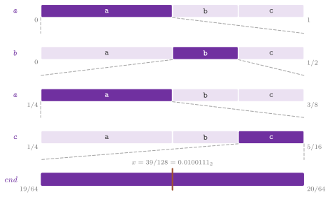
Algorithm 21.6. The interval of a text, its code, and the decoding, in exact arithmetic.
Note that the exact code needs numbers of \(d\) bits. Instead, the coder of
Witten, Neal and Cleary 1987
(RangeEncoder, the range coding of the same chapter of Ferragina) keeps
the interval in integers of \(w\) bits, \([ L , H ) \subseteq [ 0 , M )\) with
\(M = 2^w\), and we take a probability as a count out of a total \(T\). In it, the interval of a symbol of cumulative counts \([ a , b )\) is
and the intervals of the symbols tile the current one with no gap. After each symbol we expand the interval. If it lies in \([ 0 , M / 2 )\) the coder emits 0, and if it lies in \([ M / 2 , M )\) it emits 1; if it lies in \([ M / 4 , 3 M / 4 )\), straddling the middle, it emits nothing but counts an underflow, whose bit (the opposite of the next one emitted) follows that bit. In the three cases the interval is then doubled (Algorithm 21.7).
Algorithm 21.7. The encoding of a symbol and its decoding by the integer coder of Witten, Neal and Cleary 1987; \(p\) is the number of the underflows pending, and \(v\) the \(w\) bits read.
Lemma 21.4. After the expansions of
RangeEncoder::encode(), \(H - L > M / 4\); hence, with a total
\(T \le M / 4\) (the maxTotal() of the encoder and of the decoder), the interval (21.8) of a symbol of positive count is
nonempty.
Proof. When the loop of the expansions stops, none of its three cases applies, i.e., \(L < M / 2 < H\) and either \(L < M / 4\) or \(H > 3 M / 4\). In the first case \(H - L > M / 2 - M / 4\), in the second \(H - L > 3 M / 4 - M / 2\), and both are \(M / 4\). Then \(( H - L ) ( b - a ) / T > ( M / 4 ) / T \ge 1\) for \(b > a\), and the two ends of (21.8) differ by at least 1. \(\square\)
In the implementation, which follows the pseudocode, the bits are emitted by emit(), which also writes the pending underflows.
At the end, finish() emits 01 or 10, with the pending bits, according to
whether \(L < M / 4\); this picks a point of the last interval whatever bits
follow. On its side, the decoder keeps the \(w\) bits read in \(v\) and inverts (21.8) by
target(), whose result \(t\) satisfies \(a \le t < b\) for the symbol coded
(cf. Algorithm 21.7). It then applies the
same expansions to \(v\), reading zeros past the end of the code. With \(w = 32\) the rounding of (21.8) typically costs about \(10^{-4}\) bits per symbol
against the exact code, as Witten, Neal and Cleary measured.
The functions arithmeticEncode() and arithmeticDecode() code a text with a static
model of counts, whose total must not exceed \(M / 4 = 2^{w-2}\) by
Lemma 21.4
(Algorithm 21.8).
Algorithm 21.8. The arithmetic code with a static model of counts, and with the adaptive model of chapter 12 of Ferragina 2023.
An adaptive coder sends nothing in advance, which is perhaps its main convenience. It starts from \(P[ c ] = 1 / \sigma\) and, after a prefix of length \(l\) with \(l_c\) occurrences of \(c\), takes \(P[ c ] = ( l_c + 1 ) / ( l + \sigma )\). Its counts are halved, rounding up, when their total passes \(\max( 2^{16} , 2 \sigma )\), which keeps the total below \(M / 4\) and makes the model follow a text whose statistics change. Furthermore, the cumulative counts are in a tree of Fenwick 1994, where an increment, a prefix sum and the search of the symbol of a cumulative count take \(O( \log \sigma )\) time; hence a symbol costs \(O( \log \sigma )\) time, for alphabets of up to \(2^{20}\) symbols. In practice the coders typically emit bytes instead of bits (the range coder of Martin 1979), or use the asymmetric numeral systems of the next section, which reach the same compression with a multiplication or a lookup per symbol. Howard and Vitter 1994 survey the implementations in integers.
21.5 Asymmetric numeral systems¶
The asymmetric numeral systems of Duda 2013 replace the interval of the arithmetic code with a single integer state \(x\). With the frequencies \(f_c\) of the symbols scaled to a total \(M = 2^{12}\), and \(c_c\) their prefix sums (the cumulative frequency of \(c\)), the symbol \(c\) moves the state to
which multiplies \(x\) by about \(M / f_c\), i.e., adds about
\(\log_2( M / f_c )\) bits to it, the information of \(c\) under the scaled
frequencies. Conversely, the decoder reads \(c\) off \(x \bmod M\), which lies in
\([ c_c , c_c + f_c )\), and recovers the previous state. Since the decoder
undoes the last symbol first, the encoder of Rans.h takes the symbols from
the last to the first; the decoder, which reads the stream backward, then
meets them in their order.
Lemma 21.5. (i) For each \(c\), the map \(x \mapsto C( c , x )\) is a bijection of the naturals onto the naturals \(y\) with \(y \bmod M \in [ c_c , c_c + f_c )\), whose inverse is
(ii) if the encoder moves the 16 low bits of the state to the stream whenever \(x \ge 2^{20} f_c\) before (21.9), the states between two symbols stay in \([ 2^{16} , 2^{32} )\), and at most one word of 16 bits is moved per symbol.
Proof. (i) Write \(x = q f_c + r\) with \(0 \le r < f_c\). Then \(C( c , x ) = q M + c_c + r\), whose remainder modulo \(M\) is \(c_c + r \in [ c_c , c_c + f_c )\) and whose quotient is \(q\); (21.10) returns \(f_c q + r = x\), and each \(y\) with such a remainder is reached by \(x = D( y )\). (ii) Let \(2^{16} \le x < 2^{32}\). If \(x \ge 2^{20} f_c\), the state becomes \(\lfloor x / 2^{16} \rfloor\), which is at least \(2^4 f_c\) and below \(2^{16} \le 2^{20} f_c\), and a second move is not needed. Otherwise \(2^{16} \le x < 2^{20} f_c\), and \(x \ge 2^{16} \ge 2^4 f_c\) since \(f_c \le 2^{12}\). In both cases \(16 \le \lfloor x / f_c \rfloor < 2^{20}\); hence, (21.9) gives \(2^{16} \le C( c , x ) < 2^{12} \cdot 2^{20}\). After (21.10) the decoder finds a state below \(2^{16}\) if and only if the encoder had moved a word, which it reads back. \(\square\)
Hence we pay about \(\log_2( M / f_c )\) bits for a symbol, and a text about
\(\sum_i \log_2( M / f_{s[ i ]} )\) bits plus the final states. With \(f_c\)
proportional to \(n_c\) this is \(n H_0\); the rounding of the frequencies to
the total \(M\) (each byte present kept at 1 at least, by
scaleFrequencies()) costs a fraction of a percent on a text of bytes.
Unlike the arithmetic coder (cf. (21.6)), which narrows an interval and emits the bits
that its ends share, the state needs one multiplication per symbol, no
division in the decoder, and a renormalization with no carry.
Algorithm 21.9. The rANS coder of order 0 of Duda 2013 with the interleaving of Giesen 2014, and the scaling of the frequencies; \(Z[ j ]\) is the symbol of the slot \(j \in [ 0 , M )\).
Table 21.3 follows (21.9) and (21.10) on a small example, with a total \(M = 8\) in place of \(2^{12}\) and no renormalization. One can see that the state grows by about \(M / f_c\) per symbol in the encoder, and shrinks back in the decoder.
Table 21.3. rANS on the text abac with \(M = 8\), \(f_a = 4\), \(f_b = f_c = 2\) (hence \(c_a = 0\), \(c_b = 4\), \(c_c = 6\)), from the state 8: the encoder takes the symbols from the last, and the decoder reads each symbol off the state modulo 8 and undoes (21.9) by (21.10).
| Step | Encoder: \(c\) | \(x\) | \(C( c , x )\) | Decoder: \(y\) | \(y \bmod 8\) | \(c\) | \(D( y )\) |
|---|---|---|---|---|---|---|---|
| 1 | c | 8 | \(8 \cdot 4 + 6 + 0 = 38\) | 600 | 0 | a | \(4 \cdot 75 + 0 - 0 = 300\) |
| 2 | a | 38 | \(8 \cdot 9 + 0 + 2 = 74\) | 300 | 4 | b | \(2 \cdot 37 + 4 - 4 = 74\) |
| 3 | b | 74 | \(8 \cdot 37 + 4 + 0 = 300\) | 74 | 2 | a | \(4 \cdot 9 + 2 - 0 = 38\) |
| 4 | a | 300 | \(8 \cdot 75 + 0 + 0 = 600\) | 38 | 6 | c | \(2 \cdot 4 + 6 - 6 = 8\) |
Four states take the symbols in turn, \(x_{i \bmod 4}\) coding the symbol \(i\), and four chains of dependences thus overlap in the pipeline (the interleaving of Giesen 2014); the four states share one stream of words of 16 bits. In the encoder the division of (21.9) by \(f_c\) is a multiplication by a reciprocal and a shift (Granlund and Montgomery 1994), exact on the states below \(2^{32}\). Its decoder is a table of the \(M\) slots, which gives for each slot \(j\) its symbol, \(f_c\) and \(j - c_c\). We may thus write a step of it as a mask, a lookup, a multiplication and an addition, and the word of 16 bits is read with no branch, the pointer into the stream moving by twice the bit that is 1 when the state fell below \(2^{16}\).
The tabled variant of Tans.h (tANS, the entropy coder of order 0 of
Zstandard) makes the transitions of the state lookups, with no
multiplication. With \(L = 2^R\) states, \(R = 11\), and the frequencies scaled
to sum to \(L\), the \(L\) states are dealt to the symbols, \(f_c\) each, by the
step \(L / 2 + L / 8 + 3\) modulo \(L\). This step is odd, and therefore it visits all the states; also, it spreads the states of a symbol over the
table. In the state \(x \in [ 0 , L )\), the \(i\)-th state of the symbol \(c\)
(counting from 0), the decoder emits \(c\) and moves to
\(v\) being the next \(b\) bits of the stream; since \(f_c + i \in [ f_c , 2 f_c )\), one has \(( f_c + i ) 2^b \in [ L , 2 L )\) and \(x' \in [ 0 , L )\). In turn, the encoder inverts (21.11). In the state \(X \in [ L , 2 L )\) it emits the \(k\) low bits of \(X\), with \(k\) the number of bits that brings \(\lfloor X / 2^k \rfloor\) into \([ f_c , 2 f_c )\) (one of two values, found by one addition and a shift), and moves to \(L\) plus the state of the \(( \lfloor X / 2^k \rfloor - f_c )\)-th place of \(c\) (Algorithm 21.10). A symbol costs about \(\log_2( L / f_c )\) bits, and therefore the code usually comes within a fraction of a percent of \(n H_0\) when \(L\) is a few times the alphabet; Dube and Yokoo 2019 analyze the loss of the spread. We show the table of a "small" decoder in Table 21.4.
Table 21.4. The decoding table of tANS with \(L = 16\) states (\(R = 4\), step 13) for \(f_a = 8\), \(f_b = f_c = 4\): the symbol of each state, its rank \(i\) among the states of the symbol, the bits \(b\) that the decoder reads and the base \(( f_c + i ) 2^b - L\) to which it adds them.
| \(x\) | 0 | 1 | 2 | 3 | 4 | 5 | 6 | 7 |
|---|---|---|---|---|---|---|---|---|
| symbol | a | a | b | c | a | b | c | a |
| \(i\) | 0 | 1 | 0 | 0 | 2 | 1 | 1 | 3 |
| \(b\) | 1 | 1 | 2 | 2 | 1 | 2 | 2 | 1 |
| base | 0 | 2 | 0 | 0 | 4 | 4 | 4 | 6 |
| \(x\) | 8 | 9 | 10 | 11 | 12 | 13 | 14 | 15 |
| symbol | b | c | a | a | c | a | a | b |
| \(i\) | 2 | 2 | 4 | 5 | 3 | 6 | 7 | 3 |
| \(b\) | 2 | 2 | 1 | 1 | 2 | 1 | 1 | 2 |
| base | 8 | 8 | 8 | 10 | 12 | 12 | 14 | 12 |
Algorithm 21.10. The tANS coder of order 0 of Duda 2013, for one half of the text; \(\mathit{next}[ c_c + j ]\) is \(L\) plus the \(j\)-th state dealt to \(c\).
We cut the text in two halves, each with a stream of its own and four states that take its symbols in turn. A stream is written forward from the low bit of a word and read backward from its end, 4 symbols of at most 11 bits between two loads of the reader, and the two halves are decoded together; eight chains of dependences thus overlap. At the end of the stream of each half are its four final states, \(R\) bits each. Against rANS, tANS needs no multiplication (cf. (21.11)), but it needs a table per alphabet, which the encoder builds too. Both keep the static model of the frequencies in the header (2 bytes for each of the 256 bytes), and both check the header in the decoder: the frequencies sum to the total and the stream fits in the input, so that a "corrupted" input stops the decoder instead of making it read out of bounds.
21.6 Prediction by partial matching¶
So far, our models give a symbol a probability that does
not depend on the symbols before it. The prediction by partial matching
of Cleary and Witten 1984 (PPM.h,
ppmEncode() and its inverse ppmDecode()) codes each symbol arithmetically in the context of the \(K\) symbols before
it, and we follow the version C of Moffat 1990, which works as follows. For each context \(\alpha\) of length \(0 \le l \le K\)
the model counts how many times each symbol has followed \(\alpha\) in the
text seen so far. Then the symbol \(s[ i ]\) is coded in the longest context
\(s[ i - l .. i - 1 ]\) that has already seen it, starting from
\(l = \min( K , i )\). Each context on the way that does not predict it
emits an escape, whose count in the version C is the number \(q\) of the
distinct symbols seen in the context; hence a symbol of count \(c( \sigma )\)
in a context seen \(m\) times has the probability \(c( \sigma ) / ( m + q )\),
and the escape \(q / ( m + q )\). After \(K + 1\) escapes the context of order
\(-1\) gives the same probability to the symbols not yet excluded.
By the principle of exclusion, a context that escapes informs the decoder that the symbol is none of those it predicts, and the shorter contexts leave them out of their counts. Note that the escape keeps its count \(q\), as in the example of chapter 12 of Ferragina 2023; the context of order \(-1\) gives \(1 / ( \sigma - | X | )\) to each symbol outside the set \(X\) of the excluded ones, and a context whose symbols are all excluded emits nothing. After each symbol the counts of all its contexts grow by one, and those of a context are halved, rounding up, when their total passes \(2^{16}\). As usual, the decoder repeats the walk of the encoder, reading in the code whether each context escapes (Algorithm 21.11), and Table 21.5 follows the walk on a symbol.
Algorithm 21.11. The steps that code a symbol \(c\) in PPM with exclusion, version C, and the update of the counts; \(h\) is the history of the last \(K\) symbols and \(X\) the set of the symbols excluded.
Table 21.5. The steps of PPM of order \(K = 2\) on the bytes for the symbol c after abra (the fifth symbol of abracadabra): the contexts from the longest, the symbols they predict after the exclusions, the item coded and its probability.
| Context | Counts seen | Excluded before | Item coded | Probability |
|---|---|---|---|---|
| ra | none | nothing (the context is new) | 1 | |
| a | b 1 (\(q = 1\)) | escape | \(1 / ( 1 + 1 ) = 1 / 2\) | |
| (empty) | a 2, b 1, r 1 (\(q = 3\)) | b | escape | \(3 / ( 2 + 1 + 3 ) = 1 / 2\) |
| order \(-1\) | each byte 1 | a, b, r | c | \(1 / 253\) |
We see that the symbol c of Table 21.5 costs \(1 + 1 + \log_2 253 \approx 10\) bits, more than the 8 of a byte, since the model has seen only four symbols, a "small" history. Contexts typically pay off on long texts, where most symbols are coded at the first or the second context. In general, the compression approaches the entropy of order \(K\), and on the texts of a language it usually grows with \(K\) up to 4 or 5 symbols, though this may depend on the text; beyond that, the escapes cost more than the longer contexts gain, as chapter 12 of Ferragina 2023 observes. Coding a symbol takes \(O( K ( K + \sigma_K ) \log n )\) time, with \(\sigma_K\) the largest number of symbols seen in a context, since the contexts are kept in a balanced tree keyed by their strings. In practice they are kept in a trie of the contexts with links to the suffixes (Moffat 1990), where the next shorter context is a step away. Among the escape methods of the literature are A, \(1 / ( m + 1 )\), and B, \(q / m\), of Cleary and Witten 1984; C, here; D, \(q / 2 m\); P, X and XC of Witten and Bell 1991, estimated from the symbols seen once. Also, the PPMd of Shkarin 2002 estimates the escape from the statistics of similar contexts, and PPM* of Cleary, Teahan and Witten 1995 uses contexts of unbounded length.
21.7 Codes of the integers¶
The codes of IntegerCodes.h (chapter 11, Integer Coding, of
Ferragina 2023) write a sequence of
positive integers one after the other, each in a self-delimiting codeword
that is short for the small integers. We write them on the streams of bits of ADS/succinct/BitStream.h (§22.2), the most
significant bit first, and the stream thus equals the codeword on paper. By
Lemma 21.1 a code of lengths \(\ell( x )\) is
optimal for the distribution \(P[ x ] = 2^{-\ell( x )}\), and choosing a code is therefore (implicitly) choosing the distribution of the data. For instance, the d-gaps of a sorted list (its first item and the differences of consecutive items, dGaps()) are small and skewed, and a code with short codewords for
the small integers takes few bits on them. The function signedToNatural() maps an
integer of any sign to a natural number (\(x \ge 0\) to \(2 x\), \(x < 0\) to
\(-2 x + 1\)), and the codes then apply to differences of any sign.
Each code has its encoder (encodeUnary() for the unary one) and its decoder (decodeUnary(), decodeGamma(),
decodeDelta(), decodeRice(), decodeGolomb(), decodeVByte(),
decodeDense()) and the function of its length in bits or bytes
(unaryLength(), gammaLength(), deltaLength(), riceLength(),
golombLength(), vbyteLength(), denseLength()), which the encoders
ensure at the level of the postconditions; binaryLength( x ) is
\(\lvert B( x ) \rvert\), naturalToSigned() inverts signedToNatural(),
and prefixSums() inverts dGaps().
We list the codes, with their lengths and their codewords for \(x = 9\), in
Table 21.6; of course, the "optimal"
distributions of its fourth column are those of
Lemma 21.1.
Table 21.6. The codes of IntegerCodes.h;
\(B( x )\) is the binary code of \(x\), of \(\lvert B( x ) \rvert = 1 +
\lfloor \log_2 x \rfloor\) bits, and the last column the codeword of 9
(\(B( 9 ) = 1001\)).
| Code | Codeword | Length | Optimal for | \(x = 9\) |
|---|---|---|---|---|
| unary \(U( x )\) | \(0^{x - 1} 1\) | \(x\) | \(2^{-x}\) | 000000001 |
| \(\gamma\) (Elias) | \(0^{\lvert B( x ) \rvert - 1} B( x )\) | \(2 \lfloor \log_2 x \rfloor + 1\) | \(1 / ( 2 x^2 )\) | 0001001 |
| \(\delta\) (Elias) | \(\gamma( \lvert B( x ) \rvert ) \, B( x )\) | \(1 + 2 \lfloor \log_2 \lvert B( x ) \rvert \rfloor + \lvert B( x ) \rvert\) | about \(1 / ( 2 x ( \log_2 x )^2 )\) | 001001001 |
| Rice \(R_k\) | \(U( q + 1 )\), then \(r\) in \(k\) bits | \(\lfloor ( x - 1 ) / 2^k \rfloor + 1 + k\) | geometric, \(2^k \approx \ln 2 / p\) | 00100 (\(k = 2\)) |
| Golomb, modulus \(b\) | \(U( q + 1 )\), then \(r\) in truncated binary | \(q + 1 + \lfloor \log_2 b \rfloor\) or one more | \(( 1 - p )^{x-1} p\), \(b \approx \ln 2 / p\) | 00111 (\(b = 3\)) |
| variable byte | groups of 7 bits, a flag each | \(8 \lceil \lvert B( x ) \rvert / 7 \rceil\) | whole bytes | 00001001 |
| \(( s , c )\)-dense | continuers, then a stopper | \(k\) words for \(s c^{k-1}\) integers | the \(s\) of denseOptimalS() |
the word 9 (\(s = c = 128\)) |
Note that the unary code is optimal for \(2^{-x}\), and it is the part of the other codes that gives a length. Then the \(\gamma\) code of Elias 1975 writes the length of \(B( x )\) in unary, as \(\lvert B( x ) \rvert - 1\) zeros, and then \(B( x )\), whose leading 1 ends the unary part. Its decoder counts the zeros up to the first 1, a word at a time by the trailing zeros of the word, and reads as many bits more (Algorithm 21.12). In turn, the \(\delta\) code writes the length in \(\gamma\), and takes \(1 + o( 1 )\) times the bits of \(B( x )\). Chapter 11 of Ferragina keeps the leading 1 of \(B( x )\) after the length, which Elias drops since the length implies it; so do these functions, at the price of one bit more than the code of Elias.
Algorithm 21.12. The codes \(\gamma\) and \(\delta\) of Elias 1975.
We write a codeword of up to 63 bits in one field of the stream,
turned around so that its most significant bit is read first, and a longer
one by its unary part and its binary part apart. Its decoder is readUnary() followed by readBinary() of the stream
(§22.2).
The code of Golomb 1966 of modulus \(b\) writes \(x - 1 = q b + r\) as \(U( q + 1 )\) followed by the remainder \(r\) in the truncated binary code, i.e., \(\lceil \log_2 b \rceil - 1\) bits for the first \(t = 2^{\lceil \log_2 b \rceil} - b\) remainders and one more for the others. It is optimal for the geometric distribution \(( 1 - p )^{x - 1} p\) when \(b\) is about \(\ln 2 / p\) (Gallager and van Voorhis 1975), the distribution of the gaps between the occurrences of a word that occurs independently with probability \(p\). In particular, the code of Rice 1979 is the case \(b = 2^k\), whose remainder is plain binary in \(k\) bits (Algorithm 21.13).
Algorithm 21.13. The codes of Rice and of Golomb.
All these codes are decoded one bit at a time, at least in principle, while the decoders of the practice want bytes or blocks. The
variable-byte code writes \(B( x )\) in groups of 7 bits from the most
significant, each in a byte whose high bit is 1 except in the last. It is generalized by the \(( s , c )\)-dense codes of Brisaboa, Fariña, Navarro and Paramá 2007. They split the \(s + c = 2^w\) values of a word of \(w\) bits
into \(s\) stoppers, which end a codeword, and \(c\) continuers, and then \(s c^{k - 1}\) integers take \(k\) words (e.g., 128 integers take one byte when \(s = 128\)); denseOptimalS() tries each \(s\) for
given frequencies and keeps the one of the smallest output. In these terms, the variable-byte code has \(s = c = 128\), but it wastes the codewords that
begin with a group of zeros, which the dense code with \(s = c = 128\) does
not (Algorithm 21.14).
Algorithm 21.14. The variable-byte code and the dense codes.
PForDelta (Zukowski et al. 2006)
codes a block of values in \(b\) bits each after subtracting a base (the
record PForDeltaBlock, with \(b\), the base, the slots and the exceptions,
whose size() is the number of values and codeBits() the \(n b\) bits of
the slots plus 64 for each exception; decodePForDelta() decodes it). A value out of \([ \mathit{base} , \mathit{base} + 2^b - 2 ]\) is an exception, marked in its slot by the escape \(2^b - 1\) and written apart in 64 bits, and pforDeltaWidth() chooses \(b\) so that 90% of the
values fit. Its decoder unpacks the slots with no branch per value and
patches the escapes afterwards, which is, arguably, the main reason for the design. In the original the exceptions are linked in place of the escapes, and the OptPFD of
Yan, Ding and Suel 2009 chooses \(b\) for
each block by the cost of its exceptions, as patchedPack() of
§21.8 does.
The codes above take one integer at a time, while the interpolative code of
Moffat and Stuiver 2000 (encodeInterpolative(), decoded by decodeInterpolative()) takes
instead a strictly increasing sequence \(x[ l .. r - 1 ]\) in \([ \mathit{low} , \mathit{hi} ]\) at once. It writes the middle item
\(x[ m ]\), \(m = \lfloor ( l + r - 1 ) / 2 \rfloor\), in the range that the
items around it leave to it, by the binary code of the range
(encodeBounded(), decoded by decodeBounded()); then it writes the two
halves recursively, each in the
range that \(x[ m ]\) leaves it (Algorithm 21.15).
Algorithm 21.15. The interpolative code of Moffat and Stuiver 2000.
Lemma 21.6. The middle item of \(x[ l .. r - 1 ]\) lies in \([ \mathit{low} + m - l , \mathit{hi} - ( r - 1 - m ) ]\), and is written in
bits; hence a run of consecutive integers that fills its range costs no bit.
Proof. Since the \(m - l\) items before \(x[ m ]\) are distinct integers of \([ \mathit{low} , x[ m ] - 1 ]\), \(x[ m ] \ge \mathit{low} + m - l\); symmetrically, \(x[ m ] \le \mathit{hi} - ( r - 1 - m )\). Hence the range holds \(\mathit{hi} - \mathit{low} - ( r - 1 - l ) + 1\) values, whose binary code takes (21.12) bits. When the \(r - l\) items fill \([ \mathit{low} , \mathit{hi} ]\), the range of the middle item holds one value, and so does the range of each item in the recursion; one value takes 0 bits. \(\square\)
This code adapts to the clusters of a sequence, and therefore it suits the lists of an index. Since it is not a code of the items one by one (nor prefix-free item by item), it can beat the code of Huffman, which is optimal only among the static prefix-free codes of the items, at the price of a decoding that is recursive and rather slow. Finally, the code of Elias and Fano of chapter 11 of Ferragina, which is also searched in place, is in §22.6.
21.8 Engineered codes of the integers¶
The codes of §21.7 are decoded one integer at a time, each with a test of its length that the processor may not predict on "irregular" data. We now see three engineered forms that remove that test. They put the lengths apart from the bits of the integers, and a block of integers is then decoded by a fixed sequence of shifts and masks, or by one shuffle of bytes.
Binary packing. First, the SIMD-BP128 of
Lemire and Boytsov 2015
(BinaryPacking.h) cuts a sequence of integers of 32 bits into blocks of
128. It writes a block with \(b\) bits per integer, \(b\) being the bits of its
largest one, i.e., in \(16 b\) bytes, and the widths of 16 blocks are 16
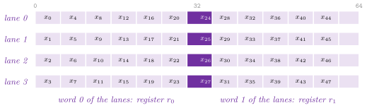
bytes before them. Inside a block the integers are laid out vertically over the
4 lanes of a register of 128 bits, the integer \(4 q + l\) in the lane \(l\) at
the bit \(q b\) of the \(32 b\) bits of the lane
(Figure 21.4). Four integers are then packed
or unpacked at once by the shifts and the masks of the four lanes,
on the lane \(l\) of the words \(w\) of the block, the second word only where
the field crosses a word. A block of each width has a separate unrolled code,
a template with each shift a constant, chosen by a table of 33 functions.
For a sorted sequence, the code is that of the differences at a distance of 4,
\(d_i = x_i - x_{i-4}\), the differential code D4 of
Lemire, Boytsov and Kurz 2016. Its decoder adds the previous register of four integers to each register it
unpacks, i.e., one addition per four integers instead of the chain of a
prefix sum, for (typically) a fraction of a bit more per integer
(Algorithm 21.16). The four lanes are those
of the vectors of Highway, with ADS_WITH_HIGHWAY on a machine of
little-endian order; without it the same layout is packed and unpacked a
lane at a time, into the same bytes.
Algorithm 21.16. The binary packing and its patched form (Lemire and Boytsov 2015).
A block takes the bits of its largest integer, to the bit, at the price of the integers that are much "larger" than the others of their block. The patched code, the PFor of Zukowski et al. 2006 in the form of the FastPFor of Lemire and Boytsov, packs a block with a width \(b\) below the width \(\beta\) of its largest integer. It writes apart the \(c( b )\) integers of \(2^b\) or more, the exceptions, as their places (a byte each) and their high bits (\(\beta - b\) each), packed after the block. Its width is the one of least cost,
where the last term is the byte of \(\beta\), which only a block with exceptions writes; the counts \(c( b )\) for all \(b\) come from the counts of the widths of the integers of the block, in one scan. On decoding, the block is unpacked as above, and then the high bits of the exceptions are set, each by a load of 8 bytes. A sorted sequence is summed at a distance of 4 in a separate pass, once its exceptions are set, since a sum read right after the scattered writes of the exceptions might wait for them to reach the cache. A block of the patched code is \(b\) and \(c\) in a byte each, \(\beta\) in a byte if \(c > 0\), the block of width \(b\), the places and the high bits; 8 bytes of 0 end the code.
Stream VByte. The variable-byte code of
§21.7 keeps the length of an integer in the bytes of the integer, a flag bit per byte, which the decoder tests one byte at a time, as we have seen.
The Stream VByte of Lemire, Kurz and Rupp 2018
(StreamVByte.h) writes each integer of 32 bits in as many bytes as its
significant bytes, \(\ell_i = \max( 1 , \lceil \mathrm{bitwidth}( x_i ) / 8
\rceil )\), and moves the lengths apart. They take 2 bits per integer: the
lengths less 1 of the integers \(4 i\), \(4 i + 1\), \(4 i + 2\) and \(4 i + 3\)
are in the bits 0-1, 2-3, 4-5 and 6-7 of the control byte \(i\), and all the
control bytes come before the data. In all, the code takes
bytes, i.e., the variable-byte code with 2 control bits per integer instead of 1 per byte. A decoder that reads a control byte knows where the four integers start, with no test on the data. With Highway, on the vectors of the processor found at run time, one shuffle of bytes moves the 16 bytes from the place of the first integer to their four places of 4 bytes, the missing high bytes made 0, with the entry of the control byte in a table of 256 masks as its mask; the place then moves by the sum of the four lengths, from a table too (Figure 21.5). The encoder finds the lengths of 4 integers at once by three comparisons of their lanes and moves their bytes by the shuffle of the inverse table. Its decoder takes 8 control bytes at a time and decodes 32 integers with no test while enough bytes follow; elsewhere the integers are moved one at a time, still with no test (Algorithm 21.17).
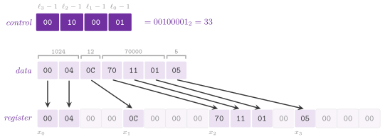
Algorithm 21.17. Stream VByte (Lemire, Kurz and Rupp 2018), one integer at a time in the encoder and four at a time in the decoder.
Directly addressable codes. None of the codes so far reads the \(i\)-th
integer without decoding the ones before it. The directly addressable
codes of Brisaboa, Ladra and Navarro 2013
(DirectAccessCodes.h) cut the bits of each integer into chunks, the low
\(b_0\) bits, the next \(b_1\), and so on. Its level \(\ell\) holds, for each integer that has bits beyond the first \(s_\ell = b_0 + \cdots +
b_{\ell - 1}\), its chunk \(\ell\) in an array \(A_\ell\) of fixed width
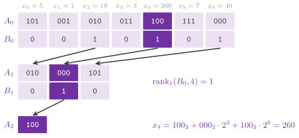
\(b_\ell\). It also holds a bit of a vector \(B_\ell\) that records whether the integer continues past the level (none on the last level). An integer at the place \(i\) of a level is at the place \(\mathrm{rank}_1( B_\ell , i )\) of
the next one, among those that continue
(Figure 21.6), and hence
over the levels that \(x_i\) reaches. Each level costs \(O( 1 )\) time with
the rank of RankSelect (§22.3), i.e., one load
of the directory and one sideways sum.
We write \(n_s\) for the integers of more than \(s\) bits (\(n_0 = n\)) and \(w\) for the bits of the largest one; then a level that holds the bits \([ s , t )\) costs \(n_s ( t - s )\) bits of chunks. Unless it is the last, it also costs \(n_s\) continuation bits, with a quarter more for their rank. Its authors find the widths that minimize the sum by a dynamic program over the places of the cuts,
Lemma 21.7. \(\mathcal{C}( 0 )\) is the least
number of bits, counted as above, of the levels of a cut of the bits
\([ 0 , w )\), and the dynamic program of DirectAccessCodes finds a cut
that attains it in \(O( w^2 )\) time from the counts \(n_s\).
Proof. A cut is a sequence \(0 = s_0 < s_1 < \cdots < s_k = w\), and its cost is a sum of terms, each of which depends only on a pair \(( s_j , s_{j+1} )\) of consecutive cuts and on whether \(s_{j+1} = w\). Hence the cheapest cut that starts at \(s\) is a first level \([ s , t )\) followed by the cheapest cut that starts at \(t\), which is (21.17). It is solved from \(s = w - 1\) down, each \(s\) by a minimum over at most \(w\) values of \(t\). \(\square\)
DirectAccessCodes reads an item by access( i ) or operator[], and is
a random-access range with the aliases of the standard containers
(value_type, size_type, difference_type, reference,
const_reference, and const_iterator, the same as iterator, with
begin(), end(), cbegin() and cend()); widths() gives the widths
of the levels and sizeInBits() the bits of the chunks, of the
continuation bits and of their ranks.
Algorithm 21.18. The construction of the directly addressable codes by (21.17), and the access (21.16) (Brisaboa, Ladra and Navarro 2013).
A fixed width \(b\) for all the levels (the second constructor) trades bits for fewer levels, i.e., for fewer ranks per access. With \(b = 7\) the chunks are those of the variable-byte code, its continuation bits moved to a separate vector with rank. A chunk of 8 or 16 bits is read as its byte or its pair of bytes, one load that stays in its line of the cache.
21.9 The compressors of Lempel and Ziv¶
The compressors of LempelZiv.h (chapter 13, Dictionary-Based
Compressors, of Ferragina 2023) need
no model of the source. Their dictionary is the text itself, and they
replace a string seen before with a reference to it. LZ77
(Ziv and Lempel 1977) parses the text
into phrases. At the place \(p\), the longest prefix \(\alpha\) of
\(s[ p .. ]\) that starts in the window of the last \(w\) symbols (and may end
past it, overlapping \(\alpha\) itself) gives the triple
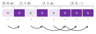
\(\langle d , \lvert \alpha \rvert , c \rangle\), with \(d\) the distance back
to the copy and \(c\) the symbol after it (none at the end of the text). Then the parse moves \(\lvert \alpha \rvert + 1\) places, and among the longest
prefixes the closest is chosen. Its decoder copies one symbol at a time, which is right on an overlapping copy too (e.g., on a run of one symbol)
(Figure 21.7).
Algorithm 21.19. The parse of LZ77 by a search of the window, and its decoding.
A search of the window takes \(O( w ( \ell + 1 ) )\) time for a phrase of
length \(\ell\), hence \(O( n w )\) in the worst case
(Lemma 21.8 below). LZSS
(Storer and Szymanski 1982,
lzssParse(), decoded by lzssDecode()) emits either a copy \(\langle d , \ell \rangle\) or a literal
\(\langle 0 , c \rangle\), a copy only if \(\ell\) reaches a minimum (1 in
chapter 13 of Ferragina, 3 in gzip). We find the copies as gzip does in lzssParseHashed(), which is perhaps the most used form of the search: the places are chained by the hash of the 3 symbols
that start there, from the most recent, and the search follows the chain of
the next 3 symbols within the window, up to a number of candidates. In this way the levels of gzip trade the length of the copies for the speed;
with no bound on the chain, the function gives the parse of lzssParse()
with minimum 3 (Algorithm 21.20). We keep the encoding of the fields of the phrases apart, and the codes of this chapter apply to them (gzip, e.g., uses a code of Huffman for the literals
and the lengths and one for the distances).
Algorithm 21.20. LZSS by the chains of the hashes of gzip.
The phrases are the records LZ77Phrase (the fields distance, length
and next, the last one empty at the end of the text), LZSSPhrase
(distance, 0 for a literal, length and literal) and LZ78Phrase
(id and next), compared field by field.
LZ78 (Ziv and Lempel 1978, lz78Parse())
keeps an explicit dictionary of phrases in a trie, which starts with the
empty phrase 0. There the longest phrase \(f\) that prefixes the rest of the text
gives \(\langle \mathit{id}( f ) , c \rangle\), and \(f c\) becomes a new
phrase; the dictionary is therefore closed under prefixes, the trie has one
symbol per edge, and a phrase costs one step of the trie per symbol. A text
that ends inside a phrase \(f\) ends with the pair of the parent of \(f\) and
its last symbol. When the dictionary has the given number of phrases it is
discarded and restarts empty (freezing it, or replacing the phrase used
least recently, are the other choices of chapter 13 of Ferragina). LZW
(Welch 1984, lzwEncode()) starts with
the 256 phrases of one byte and emits only the identifiers: the phrase \(f\)
followed by \(c\), with \(f c\) not in the dictionary, gives
\(\mathit{id}( f )\) and adds \(f c\), and the next phrase starts at \(c\)
(Algorithm 21.21).
Algorithm 21.21. LZ78 and LZW, with their decoders.
The decoder of LZW adds \(f c\) one step late, when it reads the next phrase \(f'\), whose first symbol is \(c\); the identifier of \(f'\) may then be the one of the phrase about to be added, which the decoder does not know yet. We prove that the decoders are right in this case and in the overlapping copies of LZ77, and that the dictionary of LZ78 is a trie with one symbol per edge.
Lemma 21.8. (i) The decoder of LZ77, which copies one symbol at a time, writes \(s[ p .. p + \ell - 1 ]\) for a phrase \(\langle d , \ell , c \rangle\) at the place \(p\) also when \(d < \ell\). (ii) The dictionary of LZ78 is closed under prefixes, and each phrase is a node of the trie whose parent is the phrase without its last symbol. (iii) If the decoder of LZW, after the phrase \(f\), reads the identifier of the phrase that it is about to add, that phrase is \(f\) followed by the first symbol of \(f\). (iv) The search of the window of Algorithm 21.19 costs \(O( w ( \ell + 1 ) )\) for a phrase of length \(\ell\), hence \(O( n w )\) in all.
Proof. (i) The symbol \(p + j\) is copied from \(p + j - d < p + j\), which the decoder has already written, whether it lies before \(p\) or inside the phrase; and by the definition of the phrase \(s[ p + j ] = s[ p + j - d ]\) for \(j < \ell\). (ii) The empty phrase is in the dictionary, and a new phrase \(f c\) is added only when \(f\) is in it; by induction each prefix of a phrase is a phrase, and \(f c\) is the child of \(f\) by the edge \(c\). (iii) The encoder adds \(f c\) after emitting \(f\), where \(c\) is the symbol after \(f\) in the text, and the next phrase \(f'\) starts at \(c\). If the identifier of \(f'\) is that of \(f c\), then \(f' = f c\), whose first symbol is that of \(f\); since \(f'\) also starts with \(c\), the first symbol of \(f\) is \(c\), and the phrase is \(f\) followed by its first symbol, which the decoder writes without knowing \(c\) in advance. (iv) Each of the at most \(w\) places of the window is compared with \(s[ p .. ]\) for at most \(\ell + 1\) symbols, since a match longer than \(\ell\) would give a longer phrase; the phrases cover the \(n\) symbols, and the sum of \(\ell + 1\) over them is at most \(2 n\). \(\square\)
All these compressors are universal: on the texts of an "ergodic" source
their bits per symbol tend to its entropy
(Ziv and Lempel 1978). Furthermore, the code of the \(z\) phrases of LZ78 takes at most \(n H_k + O( n \log \log n / \log n )\)
bits for each fixed \(k\) (Kosaraju and Manzini 2000),
but with a term that vanishes rather slowly. In practice LZ77 is used with long windows and "fast" searches, and with no window at all the parse is found in
\(O( n )\) time from the suffix array of the text (lz77ParseLinear() of
LZ77Linear.h). This rests on the following property of the suffixes,
which Kärkkäinen, Kempa and Puglisi 2013
exploit.
Lemma 21.9. Let \(r\) be the rank of the suffix \(i\) in \(\mathit{SA}\), and let
be the suffixes of the closest ranks before and after \(r\) that start before \(i\) (an absent one sharing no prefix with \(s[ i .. ]\)). Then the longest prefix of \(s[ i .. ]\) that starts at an earlier place has the length \(\ell( i ) = \max \{ \mathrm{lcp}( i , \mathit{PSV}( i ) ) , \mathrm{lcp}( i , \mathit{NSV}( i ) ) \}\), and it starts at the one of the two that attains the maximum.
Proof. Recall that the longest common prefix of two suffixes is the least of the longest common prefixes of the suffixes adjacent in \(\mathit{SA}\) between them, and it can therefore only decrease as the rank moves away from \(r\). Among the suffixes that start before \(i\), those of rank below \(r\) share with \(s[ i .. ]\) at most the prefix that \(\mathit{PSV}( i )\) shares, and those of rank above \(r\) at most the prefix that \(\mathit{NSV}( i )\) shares. \(\square\)
Both values of each place come from one scan of \(\mathit{SA}\) with a stack of places that increase from the bottom (lines 3 to 6 of Algorithm 21.22 below). A place pops the larger ones, of which it is the next smaller value, and the top that remains is its previous smaller value; each place is pushed and popped once.
Theorem 21.3. lz77ParseLinear() gives
the phrases of LZ77 with no window, with the lengths of lz77Parse(), in
\(O( n )\) time and two arrays of \(n\) integers of 32 bits besides the text
and the suffix array.
Proof. We first show that lines 3 to 6 of Algorithm 21.22 compute (21.18). After the scan of \(\mathit{SA}[ 0 .. j ]\), the stack holds, from the bottom, the places of \(\mathit{SA}[ 0 .. j ]\) that are smaller than each place scanned after them, in increasing order: this holds before the scan, and the place \(x = \mathit{SA}[ j + 1 ]\) removes from the set exactly the places larger than \(x\), which are at the top since the stack increases, and then enters it. A place \(y\) popped by \(x\) was smaller than each place scanned between them; hence \(x\) is the first place after \(y\) in the order of \(\mathit{SA}\) that is smaller than \(y\), i.e., \(\mathit{NSV}( y )\). The top \(z\) that remains is smaller than \(x\), and each place \(w\) scanned after \(z\) and before \(x\) is larger than \(x\): otherwise \(w\), or a place smaller than \(w\) that popped it, would be in the stack above \(z\); hence \(z = \mathit{PSV}( x )\). A place that is never popped has no next smaller value, and one that finds the stack empty has no previous one. By Lemma 21.9 the length of each phrase is then that of the longest earlier copy. Also, the scan costs \(O( n )\), and so does the suffix array of SA-IS (Nong, Zhang and Chan 2011), which is freed before the parse. At the start \(i\) of a phrase of length \(\ell\) the two longest common prefixes are found by comparing symbols, at most \(\ell + 1\) comparisons each; since the phrases cover the text, these sum to \(O( n )\). \(\square\)
Algorithm 21.22. The parse of LZ77 in linear time (Kärkkäinen, Kempa and Puglisi 2013).
Note that the source of a copy is the previous or the next smaller value, not the
closest copy that lz77Parse() chooses; the distances may therefore differ
while the lengths are the same, and the contract of the function checks
only that the phrases decode to the text. Furthermore, the parse that minimizes the bits of the code rather than the number of the phrases is studied by
Ferragina, Nitto and Venturini 2013.
LZMA, Zstandard and Brotli, in turn, add models of context and codes of the
arithmetic family to the fields of the phrases.
21.10 The transform of Burrows and Wheeler¶
The rows of the matrix \(M'\) are the \(n + 1\) rotations of \(s \$\) in sorted
order, with \(\$\) a sentinel smaller than all the symbols, \(F\) its first
column and \(L\) its last (Burrows and Wheeler 1994;
chapter 14, Block-Sorting Compression, of
Ferragina 2023). The transform
bwt() of BurrowsWheeler.h is \(L\) without the \(\$\), together with the
row \(r\) of the \(\$\) in \(L\) (the primary row), the two fields last and
primary of the record BWT. Since \(\$\) is the smallest
symbol and occurs once, sorting the rotations is sorting the suffixes, and
the symbol before the \(i\)-th smallest suffix (\(\$\) for the suffix 0). Hence the transform costs the \(O( n )\) time of the suffix array of SA-IS
(Nong, Zhang and Chan 2011, in
ADS/string/SuffixArray.h, with the suffix \(\$\) put first). Also, the rows that start with a string \(w\) are contiguous, and the symbols that precede the
occurrences of \(w\) are thus a substring of \(L\). On a text whose symbols depend on their context, as those of a language usually do, \(L\) is made of long
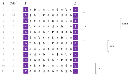
runs of few distinct symbols (Figure 21.8).
Algorithm 21.23. The transform, the LF-mapping and the inverse transform (Burrows and Wheeler 1994).
The transform can be inverted, by a property that links its two columns.
Lemma 21.10 (the LF-mapping). The \(k\)-th occurrence of a symbol \(c\) in \(L\) and the \(k\)-th occurrence of \(c\) in \(F\) are the same symbol of \(s\); hence the row
starts with the symbol \(L[ i ]\) of the row \(i\), i.e., it is the rotation of the row \(i\) by one place to the right.
Proof. Two rows \(i < j\) with \(L[ i ] = L[ j ] = c\), rotated by one place to the right, become \(c\) followed by the row \(i\) and \(c\) followed by the row \(j\) (without its last symbol), which compare as the rows \(i\) and \(j\) did. Hence the rows that start with \(c\) are in the order of the occurrences of \(c\) in \(L\), and they begin at the row \(C[ c ]\) of \(F\). \(\square\)
Lemma 21.11. Starting from the row 0, the \(n\) symbols \(L[ i_0 ] , L[ i_1 ] , \ldots , L[ i_{n-1} ]\) with \(i_0 = 0\) and \(i_{j+1} = \mathit{LF}( i_j )\) are \(s[ n - 1 ] , s[ n - 2 ] , \ldots , s[ 0 ]\); hence the inverse transform of Algorithm 21.23 gives back \(s\) in \(O( n + \sigma )\) time.
Proof. The row 0 is the rotation \(\$ s\), whose last symbol is \(s[ n - 1 ]\). By Lemma 21.10 the row \(\mathit{LF}( i )\) is the row \(i\) rotated by one place to the right, and its last symbol is therefore the symbol that precedes, in the cyclic string \(s \$\), the last symbol of the row \(i\). By induction the row \(i_j\) is \(s \$\) rotated right by \(j\) places, whose last symbol is \(s[ n - 1 - j ]\) for \(j < n\). The counts of \(L\), hence \(C\) and the ranks of (21.20) for all the rows, are found by one scan of \(L\) and a prefix sum over the \(\sigma\) symbols, and the \(n\) steps cost \(O( 1 )\) each. \(\square\)
The inverse transform thus spells \(s\) backward by \(n\) steps of (21.20), with the counts of \(L\) taken in one scan. The implementation takes the symbols of \(L\) as the bytes plus 1 and the \(\$\) as 0, and computes the LF-mapping as a counting sort of the rows by their last symbol.
Each step of the inverse is a random access to \(\mathit{LF}\), i.e., a "likely" miss of the cache on a large text; the transform is cheap to invert in operations but not (necessarily) in accesses to the memory. On the example of Figure 21.8, the row 0 ends with a, which is the first a of \(L\) and is thus mapped to the row \(\mathit{LF}( 0 ) = C[ a ] + 0 = 1\), a$abracadabr, which ends with r; and so on, until the row 3 of the \(\$\) after 11 steps.
Next come the transforms of chapter 14 of Ferragina. The move-to-front of Bentley, Sleator, Tarjan and Wei 1986 replaces each symbol with its place in a list of the alphabet, and then moves it to the front. Hence the runs of few symbols of \(L\) become runs of small integers (on the alphabet abcno, bananacocco becomes 1 1 3 1 1 1 3 4 1 0 1), in \(O( \sigma )\) time per symbol here (Algorithm 21.24).
Lemma 21.12. Writing the place \(p\) of each symbol in the move-to-front of \(s\) as \(\gamma( p + 1 )\) takes at most \(n ( 2 H_0 + 1 ) + O( \sigma \log \sigma )\) bits.
Proof. At its first occurrence a symbol has a place below \(\sigma\), which costs at most \(2 \log_2 \sigma + 1\) bits. Any other occurrence of \(c\) at the distance \(d\) from the previous one has at most \(d - 1\) distinct symbols in front of it in the list; hence \(p + 1 \le d\), and its codeword takes at most \(2 \log_2 d + 1\) bits. The \(m = n_c - 1\) distances of \(c\) sum to at most \(n\), and by the concavity of the logarithm their logarithms sum to at most \(m \log_2( n / m ) \le n_c \log_2( n / n_c ) + \log_2 e\). The sum over \(c\) is \(n H_0 + O( \sigma )\). \(\square\)
Each of the three codes of Algorithm 21.24 has its inverse,
inverseMoveToFront() (on a string or on the bytes), runLengthDecode()
and zeroRunDecode(), which the audits of the encoders apply to their
output.
Algorithm 21.24. The move-to-front and the run-length codes, as bzip2 chains them.
The run-length encoding replaces a run of \(\ell\) symbols \(c\) with \(\langle \ell , c \rangle\). In the library, bzip chains these codes as bzip2 does. First comes the transform of each block (of 900000 symbols by default), then the move-to-front of \(L\), and then the RLE0 of the runs of 0 (and of no other symbol), with the other integers grown by 1 and a run of \(m\) zeros written in the code of Wheeler (the binary digits of \(m + 1\) after its leading 1, as the symbols 0 and 1; e.g., the integers 0 0 0 0 0 3 become 1 0 4). Last comes the canonical code of Huffman of the block, with lengths up to 20, written in a preamble of 5 bits each (Algorithm 21.25). bzip2 writes the digits of the runs from the least significant one, and it splits a block in groups of 50 symbols coded by up to 6 tables, which we do not reproduce. Coding \(L\) in this way takes at most \(( 5 + \epsilon ) n H_k^*( s )\) bits plus lower terms (Manzini 2001), with \(H_k^*\) a variant of (21.2). Coding instead the pieces of \(L\) of each context of \(k\) symbols by a code of order 0 reaches \(n H_k\) plus lower terms for each \(k\) at once, which is the compression boosting of Ferragina, Giancarlo, Manzini and Sciortino 2005.
Algorithm 21.25. The decompression of bzip, each block undone in the opposite order.
21.11 Compressed indexes¶
The transform is also an index of the substrings of \(s\), which replaces
both the text and its suffix array (each index of this section gives its
space by sizeInBits())
(Ferragina and Manzini 2005). Indeed, the occurrences of a pattern \(P\) are the rows of \(M'\) prefixed by \(P\), a range
of rows, and the range can be found from \(L\) with no access to the text.
Lemma 21.13 (the backward search). If the rows prefixed by a string \(Q\) are \([ \mathit{first} , \mathit{last} )\), those prefixed by \(c Q\) are
Proof. A row is prefixed by \(c Q\) if and only if it is the image by (21.20) of a row prefixed by \(Q\) whose last symbol is \(c\). The occurrences of \(c\) in \(L[ \mathit{first} .. \mathit{last} - 1 ]\) are those of ranks \(\mathrm{rank}_c( L , \mathit{first} )\) to \(\mathrm{rank}_c( L , \mathit{last} ) - 1\) among the occurrences of \(c\) in \(L\), and by Lemma 21.10 their images are the consecutive rows that (21.21) gives. \(\square\)
Hence count( P ) of FMIndex.h applies (21.21) from the last symbol of
\(P\) to the first, \(p\) steps of two ranks each, starting from all the rows;
the occurrences are \(\mathit{last} - \mathit{first}\), found with no access
to the text (Algorithm 21.26). On the example of Figure 21.8, we see that the pattern abra goes
through the ranges \([ 1 , 6 )\) of a, \([ 10 , 12 )\) of ra, \([ 6 , 8 )\) of
bra and \([ 2 , 4 )\) of abra. The last step, from bra, is
\(C[ a ] + \mathrm{rank}_a( L , 6 ) = 1 + 1 = 2\) and \(C[ a ] +
\mathrm{rank}_a( L , 8 ) = 1 + 3 = 4\).
Algorithm 21.26. The rank in \(L\), the backward search, the location of the occurrences and the extraction of a substring in the FM-index (Ferragina and Manzini 2005).
The implementation of the search follows the pseudocode, with \(C[ c ]\) counting the \(\$\) too.
To locate the occurrences, the rows of the suffixes that start at a
multiple of \(\mu\) are marked, with their places. From any row, the
LF-mapping, which moves one place to the left in \(s\), reaches a marked row
in \(t < \mu\) steps, and the place is that of the marked row plus \(t\). Since the marks are a vector of bits with the rank of RankSelect (§22.3), a row is tested and its sample
found in \(O( 1 )\) time; the samples take \(O( ( n / \mu ) \log n )\) bits.
The function extract( i , j ) gives \(s[ i .. j - 1 ]\) from the row of the first
sampled suffix at or after \(j\), by \(j - i + O( \mu )\) steps of the
LF-mapping, each of which reads the symbol before the current suffix.
Lemma 21.14. From any row, at most \(\mu
- 1\) steps of the LF-mapping reach a marked row, and the suffix of the
starting row is the sample of the marked row plus the number of steps;
extract( i , j ) makes at most \(j - i + \mu\) steps.
Proof. By Lemma 21.10, a step from the row
of the suffix \(x \ge 1\) leads to the row of the suffix \(x - 1\). Among \(x ,
x - 1 , \ldots , x - \mu + 1\) one is a multiple of \(\mu\) (or the suffix 0
is reached first, which is a multiple of \(\mu\)), and the row of a multiple
of \(\mu\) is marked; after \(t\) steps the suffix is \(x - t\), hence \(x\) is
the sample plus \(t\). For extract(), the first sampled suffix at or after
\(j\) is below \(j + \mu\) (or it is the end of the text, the row 0), and the
steps from it down to \(i\) are at most \(j + \mu - i\); each reads the
symbol \(L\) of the current row, which precedes the current suffix.
\(\square\)
In FMIndex, the rank of a symbol in \(L\) is the count of the symbol
stored each \(b\) places for each symbol of the text, plus a scan of fewer
than \(b\) symbols, 8 at a time by the zero bytes of a word. This is \(O( b )\)
time and \(\sigma ( n / b )\) counts of 32 bits, with the defaults \(b = 64\)
and \(\mu = 32\). These counts are the simplest rank on a sequence, which a
structure of rank and select on sequences can replace
(§22.9). The wavelet tree of
Grossi, Gupta and Vitter 2003 gives the
rank in \(O( \log \sigma )\) time on \(n H_0 + o( n \log \sigma )\) bits, and
the compressed representations of
Ferragina, Manzini, Mäkinen and Navarro 2007
reach \(n H_k + o( n \log \sigma )\) bits, the space of the compressed text.
In HuffmanFMIndex.h we follow the second way, with the succinct suffix array
of Mäkinen and Navarro 2005: \(L\) is a
wavelet tree shaped by the code of Huffman (HuffmanWaveletTree,
§22.9), in \(n ( H_0 + 1 ) ( 1 + o( 1 ) )\) bits. A
step of the backward search takes the two ranks of \(c\) by one descent of
the tree along the codeword of \(c\), since both meet the same nodes, in
\(O( H_0 + 1 )\) steps on average. A step of locate() is one descent too,
since accessRank() gives \(L[ r ]\) and its rank, i.e., the LF-mapping, in
one pass. Its samples are \(\lceil n / \mu \rceil\) places and as many rows
of \(\lceil \log_2( n + 1 ) \rceil\) bits each. Its marks are \(n + 1\) bits with the compact rank of CompactRankSelect, since a step of locate() tests only the bit and the rank is needed once per occurrence. Finally,
the template parameter RS chooses the rank and select of the tree,
RankSelect for time or CompactRankSelect for space
(Algorithm 21.27).
Algorithm 21.27. The backward search and the location in the FM-index on the wavelet tree of Huffman (Mäkinen and Navarro 2005).
Also, the samples each \(\mu\) places cost \(O( ( n / \mu ) \log n )\) bits. This may be far more than \(L\) on a "repetitive" text (the versions of a document, the
genomes of a species), where the number \(r\) of the runs of \(L\) is far
smaller than \(n\). The r-index of
Gagie, Navarro and Prezza 2020
(RIndex.h) keeps \(O( r )\) words instead. \(L\) is kept as its runs: the
start \(p_j\) of each run in an Elias-Fano sequence
(§22.6), and the symbol of each run (its head
\(h_j\)) in a wavelet tree of Huffman. A further Elias-Fano sequence holds
the starts of the runs in the column \(F\), those of each symbol \(c\) after
those of the symbols before it, in one sequence of \(r\) items rather than
one for each symbol. Then the rank of \(c\) in \(L[ 0 .. i - 1 ]\) is
where \(j\) is the run of the place \(i - 1\) (one predecessor search),
\(S_c[ k ]\) the total length of the first \(k\) runs of \(c\) (read from the
starts in \(F\), where the run \(k\) of \(c\) starts at \(C[ c ] + S_c[ k ]\)), and
\(k\) the rank of \(c\) among the heads before \(j\) (one descent of the tree).
The function count( P ) is the backward search of (21.21) with it, and
Table 21.7 lists the runs of the example.
Table 21.7. The \(r = 8\) runs of the transform \(L\) = ard$rcaaaabb of abracadabra, with their first and last rows, their heads, the samples of \(\mathit{SA}\) at their two ends, and the LF-mapping of their first rows, onto which each run is shifted alike.
| Run \(j\) | Rows \([ p_j , e_j ]\) | Head \(h_j\) | \(\mathit{SA}[ p_j ]\) | \(\mathit{SA}[ e_j ]\) | \(\mathit{LF}( p_j )\) |
|---|---|---|---|---|---|
| 0 | \([ 0 , 0 ]\) | a | 11 | 11 | 1 |
| 1 | \([ 1 , 1 ]\) | r | 10 | 10 | 10 |
| 2 | \([ 2 , 2 ]\) | d | 7 | 7 | 9 |
| 3 | \([ 3 , 3 ]\) | $ | 0 | 0 | 0 |
| 4 | \([ 4 , 4 ]\) | r | 3 | 3 | 11 |
| 5 | \([ 5 , 5 ]\) | c | 5 | 5 | 8 |
| 6 | \([ 6 , 9 ]\) | a | 8 | 6 | 2 |
| 7 | \([ 10 , 11 ]\) | b | 9 | 2 | 6 |
To locate the occurrences, two properties of the suffix array on the runs replace the samples each \(\mu\) places.
Lemma 21.15 (the toehold). Let \([ \mathit{first} , \mathit{last} )\) be the rows prefixed by \(Q\), and \(v = \mathit{SA}[ \mathit{last} - 1 ]\). If \(L[ \mathit{last} - 1 ] = c\), the last row prefixed by \(c Q\) is \(\mathit{LF}( \mathit{last} - 1 )\), of the suffix \(v - 1\). Otherwise, if \(c Q\) occurs, its last row comes from the last occurrence of \(c\) in \(L[ \mathit{first} .. \mathit{last} - 2 ]\), which ends a run, and its suffix is the sample at the end of that run less 1.
Proof. By Lemma 21.13, the last row prefixed by \(c Q\) is the image of the last row \(k\) of the range with \(L[ k ] = c\). Since the LF-mapping moves one place to the left in \(s\), the suffix of the image is \(\mathit{SA}[ k ] - 1\). If \(k = \mathit{last} - 1\) this is \(v - 1\). Otherwise \(L[ k + 1 ] \ne c\), since either \(k + 1 = \mathit{last} - 1\) or \(k + 1\) is in the range after the last \(c\); hence \(k\) ends a run, whose sample is \(\mathit{SA}[ k ]\). \(\square\)
Along the backward search, then, we keep in locate( P ) the suffix of the
last row of the range (the toehold), with \(O( 1 )\) work per step beyond
the ranks. All the other occurrences follow from the function
\(\phi( \mathit{SA}[ i ] ) = \mathit{SA}[ i - 1 ]\), which lists the suffixes
of the range from the last row up.
Lemma 21.16 (the function \(\phi\)). With \(p_j\) the first row of the run \(j\),
and \(\phi( \mathit{SA}[ p_j ] ) = \mathit{SA}[ p_j - 1 ]\) is the sample at the end of the run \(j - 1\).
Proof. If the row \(i\) of \(x = \mathit{SA}[ i ]\) starts no run, then \(L[ i - 1 ] = L[ i ]\), and Lemma 21.10 maps the rows \(i - 1\) and \(i\) to adjacent rows, those of the suffixes \(\phi( x ) - 1\) and \(x - 1\). Hence \(\phi( x - 1 ) = \phi( x ) - 1\), i.e., \(\phi\) shifts \(x - 1\) and \(x\) alike. Now, the places \(x\) whose row starts a run are the \(\mathit{SA}[ p_j ]\), and (21.23) follows by induction on \(x - y\). \(\square\)
Hence one predecessor search among the \(r\) places \(\mathit{SA}[ p_j ]\),
kept sorted in an Elias-Fano sequence, gives each step of \(\phi\), together with the number \(j\) of the run (in \(\lceil \log_2 r \rceil\) bits, cf. (21.23)), whose
sample at the end of the run \(j - 1\) is \(\phi( \mathit{SA}[ p_j ] )\). On
the example, the search of ab ends on the rows \([ 2 , 4 )\) with the toehold
\(\mathit{SA}[ 3 ] = 0\). By (21.23) with \(y = 0 = \mathit{SA}[ p_3 ]\),
\(\phi( 0 )\) is the sample at the end of the run 2, i.e., 7, and the
occurrences are 0 and 7. All of it takes \(O( r )\) words: 5 sequences of
\(r\) integers of at most \(\lceil \log_2 n \rceil\) bits, and the heads, whose
rank is that of CompactRankSelect, the smallest
(Algorithm 21.28). We build the transform from the suffix array, in \(O( n )\) time and words, while in the literature the r-index is built in \(O( r )\) words from the run-length transform, which
RIndex does not attempt.
Algorithm 21.28. The construction of the r-index, the backward search on the runs, and the location by the toehold and \(\phi\) (Gagie, Navarro and Prezza 2020).
Both the LF-mapping on the runs and \(\phi\) on the places shift each
interval of a partition alike. Indeed, the LF-mapping shifts the run \(j\) onto the rows from \(\mathit{LF}( p_j )\) (cf. Table 21.7),
and \(\phi\) the stretch of places from \(\mathit{SA}[ p_j ]\) onto the places
from \(\mathit{SA}[ p_j - 1 ]\). The move structures of
Nishimoto and Tabei 2021
(§22.9) split such intervals, and the interval
of the image of a place is then found from that of the place in \(O( 1 )\)
steps. MoveRIndex.h, after the move-r of
Bertram, Fischer and Nalbach 2024,
keeps the LF-mapping as a move structure on the runs, and \(\phi\), taken
cyclically (\(\phi( \mathit{SA}[ 0 ] ) = \mathit{SA}[ n ]\)), as a move
structure on the places. This removes the predecessor searches, at the price of a few words per run, and may therefore be somewhat larger.
The backward search of MoveRIndex keeps the first and the last row of
the range, \(s\) and \(e\), with their intervals. For the symbol \(c\) it moves
\(s\) to the first row at or after it whose symbol is \(c\) (the start of the
next interval of \(c\), if its own is not of \(c\)), and \(e\) to the last one at
or before it (the end of the previous interval of \(c\)). Both moves are a
rank and a select of \(c\) on the tags of the intervals, kept in a wavelet
tree of Huffman on RankSelect; the search then maps both rows by the
LF-mapping, in \(O( 1 )\) time each. The function locate( P ) keeps \(\mathit{SA}[ e ]\)
along the search, from the samples of \(\mathit{SA}\) at the end of each
interval with the interval of \(\phi\) of each. It then lists the
occurrences by \(e - s\) steps of \(\phi\), each in \(O( 1 )\) time
(Algorithm 21.29).
Algorithm 21.29. The construction of the r-index on move structures, its count and its location (Bertram, Fischer and Nalbach 2024).
We compare the four indexes in Table 21.8. Their space and speed, measured on a common set of texts, belong to the campaign of benchmarks of Appendix B, and are not given here.
Table 21.8. The indexes of the area on a text of \(n\) bytes, for a pattern of \(p\) symbols with \(\mathit{occ}\) occurrences.
| Index | Space | count( P ) |
locate( P ), beyond the count |
|---|---|---|---|
FMIndex |
\(8 n + 32 \sigma n / b\) bits, and the samples | \(O( p b )\), a count each \(b\) places and a scan | \(O( \mathit{occ} \, \mu b )\) |
HuffmanFMIndex |
\(n ( H_0 + 1 ) ( 1 + o( 1 ) )\) bits, and the samples | \(O( p ( H_0 + 1 ) )\) on average, a descent of the tree per step | \(O( \mathit{occ} \, \mu ( H_0 + 1 ) )\) on average |
RIndex |
\(O( r )\) words | \(O( p )\) ranks on the runs, each with a predecessor search | \(O( \mathit{occ} )\) predecessor searches |
MoveRIndex |
\(O( r )\) words, a few more per run | \(O( p )\) steps of \(O( 1 )\), plus the ranks for the intervals of another symbol | \(O( \mathit{occ} )\), each in \(O( 1 )\) |
21.12 The interface¶
We collect here, header by header, the declarations of the namespace ADS
that a user calls in this chapter, without the contracts, the documentation
and the members that only the implementation uses; each block points to the
section that describes its functions, and the example at the end shows the
main structures at work. The program of the example compiles against the
headers as it stands, and its assertions hold.
// declarations of <ADS/compression/ArithmeticCoding.h>
template< class C >
std::pair< Rational , Rational >
arithmeticInterval( std::span< const C > text ,
                    const std::map< C , Rational > & prob );
template< class C >
std::string arithmeticCodeExact( std::span< const C > text ,
                                 const std::map< C , Rational > & prob );
template< class C >
std::vector< C > arithmeticDecodeExact( const std::string & bits ,
                                        std::size_t n ,
                                        const std::map< C ,
                                                        Rational > & prob );
class RangeEncoder
{
 public:
 explicit RangeEncoder( int w = 32 );
 std::uint64_t maxTotal( void ) const;
 void encode( std::uint64_t low , std::uint64_t high , std::uint64_t total );
 std::vector< std::uint8_t > finish( void );
 std::size_t bits( void ) const;
 };
class RangeDecoder
{
 public:
 explicit RangeDecoder( std::span< const std::uint8_t > bytes , int w = 32 );
 std::uint64_t maxTotal( void ) const;
 std::uint64_t target( std::uint64_t total ) const;
 void consume( std::uint64_t low , std::uint64_t high , std::uint64_t total );
 };
template< class C >
std::vector< std::uint8_t >
arithmeticEncode( std::span< const C > text ,
                  const std::map< C , std::uint64_t > & counts , int w = 32 );
template< class C >
std::vector< C >
arithmeticDecode( std::span< const std::uint8_t > code , std::size_t n ,
                  const std::map< C , std::uint64_t > & counts , int w = 32 );
std::vector< std::uint8_t >
adaptiveArithmeticEncode( std::span< const std::uint32_t > x ,
                          std::uint32_t sigma );
std::vector< std::uint32_t >
adaptiveArithmeticDecode( std::span< const std::uint8_t > code ,
                          std::size_t n ,
                          std::uint32_t sigma );
std::vector< std::uint8_t > adaptiveArithmeticEncode( std::string_view s );
std::string adaptiveArithmeticDecode( std::span< const std::uint8_t > code ,
                                      std::size_t n );
// declarations of <ADS/compression/BinaryPacking.h>
std::vector< std::uint8_t > binaryPack( std::span< const std::uint32_t > x ,
                                        bool sorted = false );
std::vector< std::uint32_t > binaryUnpack( std::span< const std::uint8_t > in ,
                                           std::size_t n ,
                                           bool sorted = false );
std::vector< std::uint8_t > patchedPack( std::span< const std::uint32_t > x ,
                                         bool sorted = false );
std::vector< std::uint32_t > patchedUnpack( std::span< const std::uint8_t > in ,
                                            std::size_t n ,
                                            bool sorted = false );
// declarations of <ADS/compression/BurrowsWheeler.h>
struct BWT
{
 std::string last;
 std::size_t primary;
 };
BWT bwt( std::string_view s );
std::vector< std::size_t > lfMapping( const BWT & b );
std::string inverseBwt( const BWT & b );
std::vector< std::uint8_t > moveToFront( std::string_view s ,
                                         std::string_view alphabet );
std::vector< std::uint8_t > moveToFront( std::string_view s );
std::string inverseMoveToFront( const std::vector< std::uint8_t > & x ,
                                std::string_view alphabet );
std::string inverseMoveToFront( const std::vector< std::uint8_t > & x );
std::vector< std::pair< std::size_t , char > >
runLengthEncode( std::string_view s );
std::string
runLengthDecode( const std::vector< std::pair< std::size_t , char > > & R );
std::vector< std::uint32_t >
zeroRunEncode( const std::vector< std::uint8_t > & x );
std::vector< std::uint8_t >
zeroRunDecode( const std::vector< std::uint32_t > & y );
std::vector< std::uint8_t > bzipCompress( std::string_view s ,
                                          std::size_t block = 900000 );
std::string bzipDecompress( std::span< const std::uint8_t > code );
// declarations of <ADS/compression/CanonicalHuffman.h>
template< class C , class F >
std::map< C , int > huffmanLengths( const std::map< C , F > & freq );
template< class C , class F >
std::map< C , int > limitedLengths( const std::map< C , F > & freq , int L );
template< class C >
class CanonicalHuffman
{
 public:
 using symbol_type = C;
 explicit CanonicalHuffman( const std::map< C , int > & lengths );
 template< class F >
 static CanonicalHuffman fromFrequencies( const std::map< C , F > & freq );
 const std::map< C , int > & lengths( void ) const;
 int maxLength( void ) const;
 std::uint64_t firstCode( int l ) const;
 std::string code( const C & c ) const;
 void encode( const C & c , PackedBitWriter & w ) const;
 std::vector< std::uint8_t > encode( std::span< const C > text ) const;
 C decode( PackedBitReader & r ) const;
 std::vector< C > decode( const std::vector< std::uint8_t > & bits ,
                          std::size_t n ) const;
 };
// declarations of <ADS/compression/DirectAccessCodes.h>
class DirectAccessCodes
{
 public:
 DirectAccessCodes( void ) = default;
 explicit DirectAccessCodes( std::span< const std::uint64_t > x );
 DirectAccessCodes( std::span< const std::uint64_t > x , int b );
 std::size_t size( void ) const;
 bool empty( void ) const;
 std::uint64_t access( std::size_t i ) const;
 std::uint64_t operator[]( std::size_t i ) const;
 std::vector< int > widths( void ) const;
 std::size_t sizeInBits( void ) const;
 using const_iterator = SubscriptIterator< DirectAccessCodes , std::uint64_t >;
 const_iterator begin( void ) const;
 const_iterator end( void ) const;
 };
// declarations of <ADS/compression/Entropy.h>
template< class C , class F >
double entropy( const std::map< C , F > & freq );
double entropy( std::string_view s );
double entropy( std::string_view s , std::size_t k );
// declarations of <ADS/compression/FMIndex.h>
class FMIndex
{
 public:
 explicit FMIndex( std::string_view s , std::size_t b = 64 ,
                   std::size_t mu = 32 );
 std::size_t size( void ) const;
 BWT transform( void ) const;
 std::size_t rank( char c , std::size_t k ) const;
 std::pair< std::size_t , std::size_t > range( std::string_view P ) const;
 std::size_t count( std::string_view P ) const;
 std::vector< std::size_t > locate( std::string_view P ) const;
 std::string extract( std::size_t i , std::size_t j ) const;
 std::size_t sizeInBits( void ) const;
 };
// declarations of <ADS/compression/HuffmanCoder.h>
std::vector< std::uint8_t >
huffmanCompress( std::span< const std::uint8_t > in );
std::vector< std::uint8_t >
huffmanDecompress( std::span< const std::uint8_t > in );
std::array< std::uint8_t , 256 >
limitedHuffmanLengths( const std::array< std::uint64_t , 256 > & f , int L );
// declarations of <ADS/compression/HuffmanFMIndex.h>
template< class RS = RankSelect >
class HuffmanFMIndex
{
 public:
 explicit HuffmanFMIndex( std::string_view s , std::size_t mu = 32 );
 std::size_t size( void ) const;
 std::pair< std::size_t , std::size_t > range( std::string_view P ) const;
 std::size_t count( std::string_view P ) const;
 std::vector< std::size_t > locate( std::string_view P ) const;
 std::string extract( std::size_t i , std::size_t j ) const;
 std::size_t sizeInBits( void ) const;
 };
// declarations of <ADS/compression/IntegerCodes.h>
constexpr int binaryLength( std::uint64_t x );
constexpr std::uint64_t signedToNatural( std::int64_t x );
constexpr std::int64_t naturalToSigned( std::uint64_t y );
std::vector< std::uint64_t > dGaps( const std::vector< std::uint64_t > & x );
std::vector< std::uint64_t >
prefixSums( const std::vector< std::uint64_t > & g );
void encodeUnary( BitWriter & w , std::uint64_t x );
std::uint64_t decodeUnary( BitReader & r );
constexpr std::uint64_t unaryLength( std::uint64_t x );
void encodeGamma( BitWriter & w , std::uint64_t x );
std::uint64_t decodeGamma( BitReader & r );
constexpr int gammaLength( std::uint64_t x );
void encodeDelta( BitWriter & w , std::uint64_t x );
std::uint64_t decodeDelta( BitReader & r );
constexpr int deltaLength( std::uint64_t x );
void encodeRice( BitWriter & w , std::uint64_t x , int k );
std::uint64_t decodeRice( BitReader & r , int k );
constexpr std::uint64_t riceLength( std::uint64_t x , int k );
void encodeGolomb( BitWriter & w , std::uint64_t x , std::uint64_t b );
std::uint64_t decodeGolomb( BitReader & r , std::uint64_t b );
constexpr std::uint64_t golombLength( std::uint64_t x , std::uint64_t b );
struct PForDeltaBlock
{
 int b = 1;
 std::uint64_t base = 0;
 BitVector slots;
 std::vector< std::uint64_t > exceptions;
 std::size_t size( void ) const;
 std::size_t codeBits( void ) const;
 };
int pforDeltaWidth( const std::vector< std::uint64_t > & x ,
                    std::uint64_t base ,
                    double f = 0.9 );
PForDeltaBlock encodePForDelta( const std::vector< std::uint64_t > & x ,
                                int b ,
                                std::uint64_t base = 0 );
std::vector< std::uint64_t > decodePForDelta( const PForDeltaBlock & p );
void encodeVByte( std::vector< std::uint8_t > & out , std::uint64_t x );
std::uint64_t decodeVByte( const std::vector< std::uint8_t > & in ,
                           std::size_t & p );
constexpr int vbyteLength( std::uint64_t x );
void encodeDense( std::vector< std::uint32_t > & out , std::uint64_t x ,
                  std::uint32_t s , std::uint32_t c );
std::uint64_t decodeDense( const std::vector< std::uint32_t > & in ,
                           std::size_t & p , std::uint32_t s ,
                           std::uint32_t c );
constexpr int denseLength( std::uint64_t x , std::uint32_t s ,
                           std::uint32_t c );
std::uint32_t denseOptimalS( const std::vector< std::uint64_t > & f ,
                             int bits = 8 );
void encodeBounded( BitWriter & w , std::uint64_t x , std::uint64_t a ,
                    std::uint64_t b );
std::uint64_t decodeBounded( BitReader & r , std::uint64_t a ,
                             std::uint64_t b );
void encodeInterpolative( BitWriter & w ,
                          const std::vector< std::uint64_t > & x ,
                          std::uint64_t low , std::uint64_t hi );
std::vector< std::uint64_t > decodeInterpolative( BitReader & r ,
                                                  std::size_t n ,
                                                  std::uint64_t low ,
                                                  std::uint64_t hi );
LempelZiv.h (§21.9).
// declarations of <ADS/compression/LempelZiv.h>
struct LZ77Phrase
{
 std::size_t distance , length;
 std::optional< char > next;
 };
struct LZSSPhrase
{
 std::size_t distance , length;
 char literal;
 };
struct LZ78Phrase
{
 std::size_t id;
 char next;
 };
std::vector< LZ77Phrase >
lz77Parse( std::string_view s ,
           std::size_t w = std::numeric_limits< std::size_t >::max() );
std::string lz77Decode( const std::vector< LZ77Phrase > & P );
std::vector< LZSSPhrase >
lzssParse( std::string_view s ,
           std::size_t w = std::numeric_limits< std::size_t >::max() ,
           std::size_t minLength = 1 );
std::vector< LZSSPhrase > lzssParseHashed(
  std::string_view s , std::size_t w , std::size_t minLength = 3 ,
  std::size_t maxChain = std::numeric_limits< std::size_t >::max() );
std::string lzssDecode( const std::vector< LZSSPhrase > & P );
std::vector< LZ78Phrase > lz78Parse(
  std::string_view s ,
  std::size_t maxPhrases = std::numeric_limits< std::size_t >::max() );
std::string lz78Decode(
  const std::vector< LZ78Phrase > & P ,
  std::size_t maxPhrases = std::numeric_limits< std::size_t >::max() );
std::vector< std::uint32_t > lzwEncode( std::string_view s );
std::string lzwDecode( const std::vector< std::uint32_t > & I );
// declarations of <ADS/compression/LZ77Linear.h>
std::vector< LZ77Phrase > lz77ParseLinear( std::string_view s );
// declarations of <ADS/compression/MoveRIndex.h>
class MoveRIndex
{
 public:
 MoveRIndex( void );
 explicit MoveRIndex( std::string_view s );
 std::size_t size( void ) const;
 std::size_t intervals( void ) const;
 std::size_t count( std::string_view P ) const;
 std::vector< std::size_t > locate( std::string_view P ) const;
 std::size_t sizeInBits( void ) const;
 };
// declarations of <ADS/compression/PackedBits.h>
class PackedBitWriter
{
 public:
 void put( bool b );
 void put( std::uint64_t v , int k );
 void put( const std::string & s );
 std::size_t size( void ) const;
 const std::vector< std::uint8_t > & bytes( void ) const;
 };
class PackedBitReader
{
 public:
 explicit PackedBitReader( std::span< const std::uint8_t > b );
 bool get( void );
 std::uint64_t get( int k );
 std::size_t position( void ) const;
 std::size_t size( void ) const;
 };
// declarations of <ADS/compression/PPM.h>
class PPMModel
{
 public:
 struct Step
 {
  std::uint64_t low , high , total;
  };
 PPMModel( int order , std::uint32_t sigma = 256 );
 int order( void ) const;
 std::uint32_t sigma( void ) const;
 std::map< std::uint32_t , std::uint64_t >
 counts( const std::vector< std::uint32_t > & ctx ) const;
 std::vector< Step > steps( std::uint32_t c ) const;
 void encode( std::uint32_t c , RangeEncoder & e ) const;
 std::uint32_t decode( RangeDecoder & d ) const;
 void update( std::uint32_t c );
 };
std::vector< std::uint8_t > ppmEncode( std::string_view s , int K );
std::string ppmDecode( std::span< const std::uint8_t > code , std::size_t n ,
                       int K );
// declarations of <ADS/compression/Rans.h>
std::vector< std::uint8_t > ransCompress( std::span< const std::uint8_t > in );
std::vector< std::uint8_t >
ransDecompress( std::span< const std::uint8_t > in );
std::array< std::uint32_t , 256 >
scaleFrequencies( const std::array< std::uint64_t , 256 > & f , int b );
// declarations of <ADS/compression/RIndex.h>
class RIndex
{
 public:
 RIndex( void );
 explicit RIndex( std::string_view s );
 std::size_t size( void ) const;
 std::size_t runs( void ) const;
 std::pair< std::size_t , std::size_t > range( std::string_view P ) const;
 std::size_t count( std::string_view P ) const;
 std::vector< std::size_t > locate( std::string_view P ) const;
 std::size_t sizeInBits( void ) const;
 };
// declarations of <ADS/compression/StreamVByte.h>
std::vector< std::uint8_t >
streamVByteEncode( std::span< const std::uint32_t > x );
std::vector< std::uint32_t >
streamVByteDecode( std::span< const std::uint8_t > code , std::size_t n );
// declarations of <ADS/compression/Tans.h>
std::vector< std::uint8_t > tansCompress( std::span< const std::uint8_t > in );
std::vector< std::uint8_t >
tansDecompress( std::span< const std::uint8_t > in );
#include "ADS/compression/CanonicalHuffman.h"
#include "ADS/compression/FMIndex.h"
#include "ADS/compression/Rans.h"
#include <cassert>
#include <string>

int main( void )
{
 const std::string s = "abracadabra";
 std::map< char , int > freq;
 for( char c : s )
  ++freq[ c ];
 const auto code = ADS::CanonicalHuffman< char >::fromFrequencies( freq );
 const std::vector< char > text( s.begin() , s.end() );
 const auto bits = code.encode( std::span< const char >( text ) );
 assert( code.decode( bits , text.size() ) == text );
 const std::span< const std::uint8_t > bytes(
   reinterpret_cast< const std::uint8_t * >( s.data() ) , s.size() );
 const auto z = ADS::ransCompress( bytes );
 const auto back = ADS::ransDecompress( z );
 assert( std::string( back.begin() , back.end() ) == s );
 const ADS::FMIndex fm( s );
 assert( ( fm.count( "abra" ) == 2 ) && ( fm.extract( 0 , 4 ) == "abra" ) );
 }
21.13 Discussion and references¶
The entropy and the bound of Lemma 21.1 are those of Shannon 1948, the optimal code of the symbols one by one is that of Huffman 1952, and the canonical code that of Schwartz and Kallick 1964. We follow the decoders by tables of Moffat and Turpin 1997; the textbook of Witten, Moffat and Bell 1999 treats them, together with the canonical code of the words of a text (the Huffword) and the indexes by inverted lists. In integers, the arithmetic code is that of Witten, Neal and Cleary 1987, the range coder that of Martin 1979, and the asymmetric numeral systems are due to Duda 2013; see also Duda et al. 2015 for their use in place of the code of Huffman. Models of context go back to Cleary and Witten 1984, with the escape methods recalled in §21.6. As for the integers, the codes are those of Elias 1975, Golomb 1966 and Rice 1979, and the survey of Pibiri and Venturini 2020 compares them with the codes by blocks on the lists of the inverted indexes.
The dictionary compressors are those of Ziv and Lempel 1977 and 1978, and the linear parses of LZ77 were also studied by Chen, Puglisi and Smyth 2008. The transform of Burrows and Wheeler 1994 became an index with the FM-index of Ferragina and Manzini 2000 and 2005. Two surveys, by Navarro and Mäkinen 2007 and by Navarro 2021, cover the compressed indexes and those of the "repetitive" texts, the latter also the r-index of Gagie, Navarro and Prezza 2018, and section 3.4.2 of Navarro 2016 treats the directly addressable codes. Chapters 11 to 14 of Ferragina 2023 are the source of the algorithms of the book. This chapter departs from them where the code departs, as remarked in place: the ceiling of (21.5), the leading 1 kept by the code \(\delta\), the order of the bits of the runs of RLE0, and the single table of bzip.
All the engineered coders of the chapter share one design. They move the lengths (of a codeword, of an integer) out of the data, or bound them, and the decoder then runs a "fixed" sequence of operations on whole words; also, they interleave "independent" streams, so that the chains of dependences of the decoder overlap. How much each of these choices may gain, against the plain forms of the book and against the implementations of reference, is measured by the campaign of Appendix B, and no number is given here.
The compressed indexes of §21.11 (FMIndex,
HuffmanFMIndex, RIndex and MoveRIndex) are persistent
(§23.7). An index of a text or of a collection of
genomes, whose construction costs a suffix array, may thus be written once
and then opened in place by restoreMapped(), with its vectors of bits and
its wavelet trees as views over the mapping. We remark that an r-index read
from a file has no copy of its text; under the contracts of level 3, the
audit of locate() against the text is then skipped.
21.14 Exercises¶
Each exercise names the test of the library that solves it (run it with
ctest -R <name>).
- Compute the empirical entropy of order 0 and of order \(k\) of a string,
and check that \(H_k \le H_0\) on random strings. Test:
pearls_compression.entropy. - Build the canonical code of given lengths, with the first codewords
(21.5) rounded up, and decode a codeword by the values
\(\mathit{fc}[ l ]\); check it on the lengths of
Figure 21.1. Tests:
pearls_compression.canonical-huffman-notes,pearls_compression.canonical-huffman. - Bound the lengths of a code of Huffman by the iterative halving of the
frequencies, and prove that it ends
(Lemma 21.3). Test:
pearls_compression.limited-lengths. - Code a string of bytes with the optimal lengths of at most 11 bits found
by package-merge, and decode it by a table of up to 3 symbols a lookup
on four interleaved streams. Test:
engineered_succinct.huffman-coder. - Compute the arithmetic code of abac in exact arithmetic
(Figure 21.3), and check that its length
is within 2 bits of \(n H_0\) on random texts. Test:
pearls_compression.arithmetic-exact. - Realize the integer arithmetic coder with the underflows, prove
Lemma 21.4, and code a text with a static
model and with the adaptive model on a tree of Fenwick. Tests:
pearls_compression.range-coder-notes,pearls_compression.arithmetic-static,pearls_compression.arithmetic-adaptive. - Realize rANS with four interleaved states and the renormalization of
Lemma 21.5, and make the decoder stop on
a corrupted input instead of reading out of bounds. Tests:
engineered_succinct.rans-coder,engineered_succinct.rans-corrupted. - Realize tANS with the spread of the states by the step
\(L / 2 + L / 8 + 3\) and two halves of four states each. Test:
engineered_succinct.tans-coder. - Realize PPM with exclusion, version C, and follow the steps of
Table 21.5. Tests:
pearls_compression.ppm-notes,pearls_compression.ppm. - Write the codes unary, \(\gamma\), \(\delta\), Rice, Golomb, PForDelta,
variable byte, \(( s , c )\)-dense and interpolative, each with its
length function, and check them on the codewords of
Table 21.6. Tests:
pearls_succinct.elias-codes,pearls_succinct.rice-golomb,pearls_succinct.pfordelta,pearls_succinct.vbyte-dense,pearls_succinct.interpolative,pearls_succinct.signed-gaps. - Pack blocks of 128 integers vertically in four lanes, with the
differences at a distance of 4 for the sorted sequences, and with the
width of least cost (21.14) of the patched code; check that the scalar
layout is the same as the vectorial one. Tests:
engineered_succinct.binary-packing,succinct_top.binary-packing-scalar. - Realize Stream VByte, with the lengths in control bytes and a decoder
that moves four integers by one shuffle. Test:
engineered_succinct.stream-vbyte. - Realize the directly addressable codes with the widths of
(21.17), and access an item in time proportional to its length. Test:
engineered_succinct.direct-access-codes. - Parse a text by LZ77 (with and without a window), LZSS (by a search of
the window and by the chains of the hashes of gzip), LZ78 and LZW, and
decode each parse. Tests:
pearls_compression.lz77-notes,pearls_compression.lz77,pearls_compression.lz78,pearls_compression.lzw. - Compute the parse of LZ77 with no window in \(O( n )\) time by the
previous and the next smaller values of the suffix array
(Theorem 21.3). Test:
engineered_succinct.lz77-linear. - Compute the transform of Burrows and Wheeler and invert it by the
LF-mapping; chain the move-to-front, RLE0 and a canonical code of
Huffman into a bzip. Tests:
pearls_compression.bwt-notes,pearls_compression.bwt,pearls_compression.mtf-rle,pearls_compression.bzip. - Count, locate and extract by the FM-index, and follow the backward
search of Figure 21.8. Tests:
pearls_compression.fm-index-notes,pearls_compression.fm-index. - Realize the FM-index on the wavelet tree of Huffman of \(L\), with the
LF-mapping of a step of
locate()in one descent. Test:engineered_succinct.huffman-fm-index. - Realize the r-index, with the rank on the runs (21.22), the toehold
and the function \(\phi\) (Lemma 21.15
and Lemma 21.16), and then replace its
predecessor searches with move structures. Tests:
engineered_succinct.r-index,engineered_succinct.move-r-index.