15. Strings¶
[Source: include/ADS/string/StringMatching.h, StringSearch.h,
AhoCorasick.h, MultiSearch.h, ApproximateMatching.h,
LongestCommonSubsequence.h, Alignment.h, SubsequenceProblems.h,
EditDistance.h, SuffixArray.h, SuffixSorting.h, SuffixTree.h,
SuffixAutomaton.h, SuffixApplications.h, LongestCommonExtension.h,
PrefixSearch.h, FrontCoding.h, RearCoding.h, Palindromes.h,
Lyndon.h, Parentheses.h, Anagrams.h, WordBreak.h,
Segmentations.h, StringBreaking.h, Huffman.h]
We are concerned in this chapter with the algorithms and the data
structures on strings: the search of one pattern and of many in a text,
the comparison of two strings by dynamic programming (the edit distance,
the longest common subsequence and the alignments), the indexes of a text
built on its suffixes, the dictionaries of strings searched by prefix, a
few combinatorial problems (palindromes, Lyndon words, parentheses,
anagrams), and the problems of segmentation and of coding that chapters 13
and 14 of Montresor 2025 solve by
dynamic programming or by a greedy choice. Most of the headers beyond that
book follow chapters 9 and 10 of Ferragina
2023, on searching strings by prefix
and by substring. For several problems the area has two layers: the
algorithm of the textbooks, which the tests use as a reference, and an
engineered realization of the same specification. §15.1
fixes the notation. §15.2 and
§15.3 treat the exact search of one pattern and
of many, and §15.4 the edit distance and its
relatives. We treat the suffix arrays, trees and automata, with their applications,
in §15.5, and the dictionaries searched by
prefix in §15.6. Finally,
§15.7 and §15.8
collect the combinatorial problems, the segmentations, the cuts of a
string and the code of Huffman. In the sets of
§1.9, AhoCorasick.h, EditDistance.h,
LongestCommonExtension.h, MultiSearch.h, StringSearch.h,
SuffixAutomaton.h and SuffixSorting.h are advanced and the other
headers of this chapter are base.
15.1 Definitions and notation¶
An alphabet \(\Sigma\) is a finite set of \(\sigma\) symbols with a total
order: the bytes of a std::string_view (\(\sigma \le 256\), compared as
unsigned values), or the integers in \([ 0 , K )\) of a vector of Symbols.
A string \(T = T[ 0 .. n - 1 ]\) of length \(n = | T |\) is a sequence of \(n\)
symbols, the places counting from 0 as in the code (both books count from
1, and the headers say where they translate). For \(0 \le i \le j < n\) the
string \(T[ i .. j ]\) is a substring of \(T\), a prefix if \(i = 0\) and a
suffix if \(j = n - 1\). We call the suffix that starts at \(i\) the
suffix \(i\), or \(T[ i .. ]\), and \(T( i ) = T[ 0 .. i - 1 ]\) is the prefix
of \(i\) symbols of Montresor 2025.
A subsequence keeps some of the symbols in their order, not necessarily
contiguous. Two strings are compared in the lexicographic order, a string
that is a prefix of another being the smaller. We call terminator the symbol \(\$\) that
some structures append, a symbol smaller than all the others, so that no
suffix of \(T \$\) is a prefix of another; Table 15.1
lists the other symbols that recur in the chapter.
Table 15.1. The symbols of the headers of
ADS/string.
| Symbol | Meaning |
|---|---|
| \(T\), \(n\); \(P\), \(m\) | the text and its length; the pattern and its length (\(P_0 , \ldots , P_{k-1}\) for \(k\) patterns of \(M\) symbols in all) |
| \(\mathrm{Occ}( P , T )\), \(\mathit{occ}\) | the places \(s \in [ 0 , n - m ]\) with \(T[ s .. s + m - 1 ] = P\), and their number |
| \(\mathrm{lcp}( x , y )\), \(\mathrm{lce}( i , j )\) | the length of the longest common prefix of two strings, and that of the suffixes \(i\) and \(j\) of one text (their longest common extension) |
| \(\mathit{SA}\), \(\mathit{SA}^{-1}\), \(\mathit{LCP}\) | the suffix array, its inverse (the rank of each suffix), and \(\mathit{LCP}[ r ] = \mathrm{lcp}( T[ \mathit{SA}[ r ] .. ] , T[ \mathit{SA}[ r + 1 ] .. ] )\), \(n - 1\) entries |
| \(F[ q ]\) | the failure function, the length of the longest proper border of \(P[ 0 .. q - 1 ]\) |
| \(D[ i ][ j ]\), \(\mathit{DP}[ i ][ j ]\) | a table of dynamic programming on the prefixes of \(i\) symbols of a string and of \(j\) of another |
| \(d\), \(k\) | the edit distance of two strings, and a bound on it (the errors or mismatches allowed) |
| \(w\) | the length of a machine word, 64 bits |
A border of a string is a string that is both a proper prefix and a proper suffix of it, and a period of \(P\) is an integer \(p > 0\) with \(P[ i ] = P[ i + p ]\) wherever both sides are defined. The edit distance (of Levenshtein 1966) of two strings is the least number of substitutions, insertions and deletions of single symbols that turn one into the other. Borders and periods are two views of the same object, as the following elementary lemma states.
Lemma 15.1. An integer \(0 < p \le m\) is a period of \(P\) if and only if \(P[ 0 .. m - p - 1 ]\) is a border of \(P\) (the empty string for \(p = m\)); hence the smallest period of \(P\) is \(m - F[ m ]\).
Proof. \(P[ i ] = P[ i + p ]\) for \(0 \le i < m - p\) says exactly that the prefix of \(m - p\) symbols equals the suffix of \(m - p\) symbols. The longest border, of length \(F[ m ]\), thus gives the smallest period. \(\square\)
15.2 The search of one pattern¶
We want to find \(\mathrm{Occ}( P , T )\); by convention the empty
pattern occurs at every place \(0 , \ldots , n\). Trying all the shifts of \(P\)
along \(T\) costs \(O( n m )\) comparisons (naiveMatching()), and the
algorithms of StringMatching.h differ in how much they learn from a
comparison and how far they then move the pattern. These are the
algorithms of the textbooks, several of which count their comparisons on
request; the engineered search of the library is StringSearcher
(§15.2.2).
15.2.1 The algorithms of the textbooks¶
Knuth, Morris and Pratt. Suppose that the prefix \(P[ 0 .. q - 1 ]\) matches the text up to the place \(i - 1\) and that \(P[ q ] \ne T[ i ]\). Moving the pattern by one place, the naive algorithm compares again symbols of the text that it has already read; however, what it would find is determined by \(P\) alone, as the next lemma shows.
Lemma 15.2. If \(P[ 0 .. q - 1 ] = T[ i - q .. i - 1 ]\) and \(P[ q ] \ne T[ i ]\), no occurrence of \(P\) starts at a place \(s\) with \(i - q < s < i - F[ q ]\), and an occurrence that starts at \(i - F[ q ]\) has \(P[ 0 .. F[ q ] - 1 ]\) already matched; hence the search can go on with
Proof. An occurrence at \(s = i - q + t\), with \(0 < t < q - F[ q ]\), would give \(P[ 0 .. q - t - 1 ] = T[ s .. i - 1 ] = P[ t .. q - 1 ]\), i.e., a border of \(P[ 0 .. q - 1 ]\) of length \(q - t > F[ q ]\), against the definition of \(F[ q ]\). At \(s = i - F[ q ]\), the first \(F[ q ]\) symbols of \(P\) are the border, which matches \(T[ i - F[ q ] .. i - 1 ]\). \(\square\)
In the algorithm of Knuth, Morris and Pratt
1977 (kmp()) we apply (15.1) at each
mismatch, with \(F[ 0 ] = -1\) meaning that \(T[ i ]\) matches no prefix, and
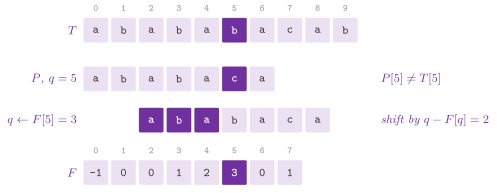
the scan never moves back in the text (Figure 15.1,
Algorithm 15.1). We compute the failure function
by the same scan of \(P\) against itself, as the next lemma justifies.
Lemma 15.3. The borders of
\(P[ 0 .. q - 1 ]\) have the lengths \(F[ q ] , F[ F[ q ] ] , \ldots\), down to
0, and \(F[ q + 1 ] = b + 1\) for the largest \(b\) in this chain with
\(P[ b ] = P[ q ]\), or 0 if there is none; hence failure() computes \(F\).
Proof. A border of a border of \(x\) is a border of \(x\), and a border of
\(x\) shorter than the longest one, of length \(F\), is a border of that
longest border, since both are prefixes and suffixes of \(x\); by induction
the chain lists all the borders, in decreasing order. A nonempty border of
\(P[ 0 .. q ]\) is a border \(P[ 0 .. b - 1 ]\) of \(P[ 0 .. q - 1 ]\) followed by
\(P[ b ] = P[ q ]\), and conversely; the longest one comes from the largest
such \(b\) of the chain. In failure() we follow the chain from
\(F[ q ]\) until we find such a \(b\), i.e., we apply this rule.
\(\square\)
Algorithm 15.1. The failure function and the search of Knuth, Morris and Pratt 1977.
Theorem 15.1. kmp() reports
\(\mathrm{Occ}( P , T )\) with at most \(2 n\) comparisons of symbols, after
the computation of \(F\) with at most \(2 m\); hence in \(\Theta( n + m )\)
time.
Proof. Correctness follows from Lemma 15.2, and from the same lemma applied after an occurrence (with \(q = m\)). Each comparison of line 4 either succeeds, and then \(i\) advances, or fails, and then the start \(i - q\) of the pattern moves forward by \(q - F[ q ] > 0\); both \(i\) and \(i - q\) are at most \(n\) and never decrease and hence there are at most \(2 n\) comparisons. By the same argument on \(P\) against itself one bounds the computation of \(F\). \(\square\)
We keep apart the function that line 4 of kmp() follows at a mismatch and the value
\(F[ m ]\) that line 6 follows after an occurrence, so that
the same loop serves the strong variant below, which changes only the
former.
Note that when \(P[ F[ q ] ] = P[ q ]\), the comparison that (15.1) makes
after a mismatch on \(P[ q ]\) fails again. The strong failure function of Knuth
skips such borders, \(G[ q ] = G[ F[ q ] ]\) if \(P[ F[ q ] ] = P[ q ]\) and
\(G[ q ] = F[ q ]\) otherwise (strongFailure()), and kmpStrong() follows
\(G\) at a mismatch, and it thus never compares a symbol of \(T\) twice with the
same symbol of \(P\); the bound of Theorem 15.1
does not change.
Boyer and Moore, Horspool. The algorithm of Boyer and Moore
1977 (boyerMoore()) compares the
window from right to left and, at a mismatch, moves it by the larger of
two shifts that pass no occurrence. By the bad character rule we align the
symbol of \(T\) that failed with its last place in \(P\) (or move the pattern
past it); by the strong good suffix rule we align the suffix already matched
with its previous occurrence in \(P\) preceded by another symbol (or with
the longest prefix of \(P\) that is a suffix of it). Both are prepared in
\(O( m + \sigma )\) time. A shift is safe since any smaller one would put a
different symbol under a symbol of \(T\) already read. When the symbols of
\(T\) seldom occur in \(P\), the window moves by about \(m\) after a few
comparisons, i.e., \(O( n / m )\) comparisons at best. Yet, the worst case
for all the occurrences is \(O( n m )\), e.g., each of the \(n - m + 1\)
windows of \(a^m\) in \(a^n\) is read whole (for the first occurrence alone
the strong good suffix rule gives \(O( n )\), as Knuth, Morris and Pratt
1977 prove). Horspool 1980
(horspool()) keeps only the bad character of the last symbol of the
window,
which is simpler and often (but not always) faster on large alphabets, with the same worst case.
Shift-Or. The bit-parallel algorithm of Baeza-Yates and Gonnet
1992 (shiftOr(), \(m \le 64\))
keeps in one word \(D\) the prefixes of \(P\) that end at the current symbol:
the bit \(i\) of \(D\) is clear when \(P[ 0 .. i ] = T[ j - i .. j ]\). Since
\(P[ 0 .. i ]\) ends at \(j\) exactly when \(P[ 0 .. i - 1 ]\) ends at \(j - 1\)
and \(P[ i ] = T[ j ]\), all the bits are updated at once by
where the bit \(i\) of \(B[ c ]\) is clear when \(P[ i ] = c\), and an occurrence ends at \(j\) when the bit \(m - 1\) of \(D\) is clear.
Lemma 15.4. Starting from \(D\) with all
the bits set, after (15.3) on \(T[ j ]\) the bit \(i < m\) of \(D\) is clear if
and only if \(P[ 0 .. i ] = T[ j - i .. j ]\); hence shiftOr() reports
\(\mathrm{Occ}( P , T )\) in \(\Theta( n )\) operations on words after a
preparation of \(O( m + \sigma )\).
Proof. By induction on \(j\). We see that the shift brings the bit \(i - 1\) of the old \(D\) to the place \(i\) and clears the bit 0, and the OR with \(B[ T[ j ] ]\) sets the bit \(i\) unless \(P[ i ] = T[ j ]\). Hence the bit \(i\) is clear if and only if \(P[ i ] = T[ j ]\) and either \(i = 0\) or the old bit \(i - 1\) was clear, i.e., by the induction (or the start, for \(j = 0\)), \(P[ 0 .. i - 1 ] = T[ j - i .. j - 1 ]\). The table \(B\) costs \(O( m + \sigma )\), and each symbol of \(T\) one shift, one OR and one test. \(\square\)
Z-function. The Z-function of a string \(S\) of \(n\) symbols is
\(Z[ i ] = \mathrm{lcp}( S , S[ i .. ] )\) (zFunction(), with
\(Z[ 0 ] = n\)), and the occurrences of \(P\) in \(T\) are the places where the
Z-function of \(P\) joined to \(T\) reaches \(m\) (zMatching() extends the
boxes of \(T\) against \(P\) in the same way, without building the join). Its
computation reuses what it has already compared, as the next lemma shows.
Lemma 15.5. Let \([ l , r )\) be the
Z-box, i.e., the interval \([ i' , i' + Z[ i' ] )\) with \(i' < i\) that
reaches farthest. If \(i < r\), then \(Z[ i ] \ge \min( Z[ i - l ] , r - i )\),
with equality when \(Z[ i - l ] < r - i\); hence zFunction() takes
\(\Theta( n )\) time.
Proof. \(S[ l .. r - 1 ] = S[ 0 .. r - l - 1 ]\), and therefore \(S[ i .. r - 1 ] = S[ i - l .. r - l - 1 ]\), and the common prefix of \(S\) and \(S[ i - l .. ]\), cut at \(r - i\), is also one of \(S\) and \(S[ i .. ]\); when \(Z[ i - l ] < r - i\) the mismatch that ends it lies inside the box too. Only the symbols past \(r\) are then compared: each successful comparison moves \(r\) forward, which happens at most \(n\) times, and each \(i\) has at most one failed comparison. \(\square\)
Two-Way. The algorithm of Crochemore and Perrin
1991 (twoWay()) has the linear
bound of Theorem 15.1 in \(O( 1 )\) extra space. It
cuts the pattern as \(P = u v\) at a critical factorization, whose local
period at the cut (the least \(q\) such that \(u\) and \(v\) agree with a shift
of \(q\) around the cut) equals the period \(p\) of \(P\). By the critical
factorization theorem (of Césari and Vincent, in the form of Crochemore
and Perrin 1991) such a cut exists
with \(| u |\) smaller than \(p\), and the later of the two maximal suffixes of
\(P\), for an order of the symbols and for its reverse, gives one. Then the
search compares \(v\) from left to right and then \(u\) from right to left
(Algorithm 15.2). A mismatch in \(v\) at the place
\(i\) moves the window by \(i - | u | + 1\), leaving behind each symbol of \(T\)
read in \(v\); a mismatch in \(u\), or an occurrence, moves it by \(p\). When
\(P\) is periodic (i.e., \(u\) is a suffix of \(P[ 0 .. p + | u | - 1 ]\)), the
prefix of \(P\) known to match after such a shift is remembered in \(\mu\), and
otherwise the shift is \(\max( | u | , | v | ) + 1\). By the critical
factorization neither shift passes an occurrence, and the algorithm makes
at most \(2 n\) comparisons, as the next lemma states.
Lemma 15.6. (Crochemore and Perrin 1991.) Let \(P\) be a nonempty string on a totally ordered alphabet, \(p( x )\) the period of a string \(x\), and \(P = u v\) with \(v\) the shorter of the two maximal suffixes of \(P\), for the order of the symbols and for its reverse. Then (i) \(u v\) is a critical factorization, i.e., its local period equals \(p( P )\), and \(| u | < p( P )\); (ii) if \(u\) is a suffix of \(v[ 0 .. p( v ) - 1 ]\), then \(p( P ) = p( v )\), and otherwise \(p( P ) > \max( | u | , | v | )\); (iii) with these \(u\), \(v\) and shifts, the search of Algorithm 15.2 reports each occurrence of \(P\) in \(T\), and only those, in at most \(2 n\) comparisons of symbols.
Proof. Part (i) is the critical factorization theorem of the paper,
with the choice of the shorter maximal suffix proved there; part (ii) and
the correctness and the cost of the search are proved there for the search
as written in Algorithm 15.2, with the memory
\(\mu\) in the first case and the shift \(\max( | u | , | v | ) + 1\) in the
second. We check the hypotheses against the code. The symbols are bytes,
compared as unsigned char, a total order, and maximalSuffix() runs the
procedure of the paper for that order and, with its flag, for the reverse
one, and returns the start of the maximal suffix and the period of that
suffix; the code takes the later start (the shorter suffix) as \(\ell + 1 = |
u |\), with its period \(p( v )\). Its test \(P[ 0 .. \ell ] = P[ p .. p + \ell
]\) is the condition of (ii), since \(| u | = \ell + 1\) and the suffix of
length \(| u |\) of \(v[ 0 .. p - 1 ]\) is \(P[ p .. p + \ell ]\), which lies in
\(P\) because \(p( v ) \le | v |\). Finally, the code shifts by \(i - \ell\)
after a mismatch at the place \(i\) of \(v\), by \(p\) after the scan of \(u\), and
sets \(\mu = m - p - 1\) only in the first case, as the algorithm of the
paper. \(\square\)
Algorithm 15.2. The Two-Way algorithm (Crochemore and Perrin 1991); \(\ell = | u | - 1\), and \(\mu\) is the last place of the prefix of \(P\) known to match (\(-1\) if none).
Table 15.2 summarizes the algorithms of the textbooks and the engineered search of the next section.
Table 15.2. The algorithms of the search of one pattern.
| Function | Preparation | Search, worst case | Remarks |
|---|---|---|---|
naiveMatching() |
none | \(O( n m )\) | \(O( n )\) expected on random texts |
kmp(), kmpStrong() |
\(O( m )\) | at most \(2 n\) comparisons | never moves back in \(T\) |
boyerMoore(), horspool() |
\(O( m + \sigma )\) | \(O( n m )\) | \(O( n / m )\) comparisons at best |
shiftOr() |
\(O( m + \sigma )\) | \(\Theta( n )\) word operations | \(m \le 64\) |
zMatching() |
\(O( m )\) | \(\Theta( n + m )\) | the Z-boxes of \(T\) against \(P\) |
twoWay() |
\(O( m )\) | at most \(2 n\) comparisons | \(O( 1 )\) extra space |
StringSearcher |
\(O( 256 + m )\) | \(O( n + m )\) | filters of probes or of q-grams |
15.2.2 The engineered search¶
We now turn to the engineered search. StringSearcher of StringSearch.h prepares the pattern once, as the
searchers of std::search() do, and then finds its occurrences in any
text; find() gives the first one at or after a place, findAll() all of
them in increasing order (overlapping ones included), and count() their
number. It chooses among three methods by the length of the pattern
(Algorithm 15.3).
First, a pattern of one byte is found by memchr(). Second, a pattern of
fewer than kSkip \(= 64\) bytes goes through a filter of probes (the packed
filters of Faro and Kulekci 2013 and of
Mula 2016): with
\(o_1 , \ldots , o_k\) the places of the \(k\) rarest bytes
\(b_i = P[ o_i ]\) of \(P\), the start \(s\) is compared with \(P\) by memcmp()
only if \(T[ s + o_i ] = b_i\) for each \(i\). Here \(k = 2\), or \(k = 4\) when
\(P\) hints at a small alphabet (fewer than 8 distinct bytes in 8 or more,
or a repeated byte in fewer, as on DNA), and the rarest bytes are those of
a fixed ranking of the bytes by their frequency in text, the later place
on a tie. This test is made for \(W\) consecutive starts at once by \(k\)
vector comparisons of \(W = 32\) bytes and their AND, by the vectors of
Highway inlined at the instructions of the compiler; without Highway
memchr() finds
the first probe and the others are checked one by one. On a text of
independent bytes of probabilities \(p_c\), the expected number of
comparisons with \(P\) is \(( n - m + 1 ) \prod_i p_{b_i}\), e.g., about
\(n / 256\) on DNA with four probes.
Third, a pattern of 64 bytes or more is searched by the shifts of its q-grams, in the spirit of Horspool 1980 and of Wu and Manber 1994, as the hashed q-grams of Lecroq 2007. We take as the length \(q\) the least one with \(d^q \ge 16 m\) for the \(d\) distinct bytes of \(P\), \(2 \le q \le 8\); a q-gram \(g\) is hashed to \(h( g ) \in [ 0 , 4096 )\) (the 12 top bits of its product by \(\lfloor 2^{64} / \phi \rfloor\), \(\phi\) the golden ratio), and
with 0 for the hash of the last q-gram of \(P\). Thus the window at \(s\) moves to \(s + \mathit{shift}[ h( T[ s + m - q .. s + m - 1 ] ) ]\), and a window of shift 0 is compared with \(P\) and then moves by the shift that the last q-gram of \(P\) has among the others. No shift passes an occurrence.
Lemma 15.7. Let the window at \(s\) end with the q-gram \(g\), and \(\delta\) be its shift by (15.4). No occurrence of \(P\) starts at a place \(s'\) with \(s < s' < s + \delta\).
Proof. Such an occurrence holds \(g\) at the place \(i = m - q - ( s' - s )\) of \(P\), with \(0 \le i < m - q\) since \(1 \le s' - s < \delta \le m - q + 1\). Then \(h( P[ i .. i + q - 1 ] ) = h( g )\), and (15.4) gives \(\delta \le m - q - i = s' - s\), a contradiction; the bound 255 and the collisions of \(h\) only make \(\delta\) smaller. The shift after a comparison is that of the same \(g\) among the q-grams of \(P\) other than its last, and the same argument applies. \(\square\) On random texts a window moves by about \(m - q + 1\), i.e., \(O( n / m )\) windows of one load of 8 bytes each; the text is prefetched 1024 bytes ahead, and the four quarters of a text of 16 KB or more are searched at once, whence the chains of loads of the four overlap. When 64 steps have moved the first window by less than \(16 m\) (a text of few distinct q-grams), the filter of the probes takes over.
Algorithm 15.3. The search of
StringSearcher, with the preparation of the shifts (15.4) and of the
probes.
Both filters may let through many windows that are not occurrences (say,
a pattern that agrees with a periodic text on its probes and nowhere
else), and the comparisons with \(P\) would then cost \(\Theta( n m )\), as
they would for \(a^m\) in \(a^n\), which occurs at every place. Each search
therefore counts the bytes of its comparisons with \(P\), those that find an
occurrence included, and line 12 hands the rest of the text to the Two-Way
algorithm once they exceed \(16 ( s - s_0 ) + 4096\) at the window \(s\) of a
search begun at \(s_0\). In this fallback the Two-Way algorithm compares 8 bytes at a time in
both directions, and its factorization (\(O( m )\)), the same function
criticalFactorization() that twoWay() calls, is computed only when a
search comes to it.
Lemma 15.8. StringSearcher::findAll()
takes \(O( n + m )\) time on any text, after a preparation of
\(O( 256 + m )\) time and 4 KB of space.
Proof. Before the switch the filters cost \(O( 1 )\) per window and the comparisons at most \(16 n + 4096 + m\) bytes; after it the Two-Way algorithm makes at most \(2 n\) comparisons, plus \(O( m )\) for its factorization. Neither filter misses an occurrence, as remarked above. \(\square\)
Besides find(), findAll() and count(), the searcher answers
operator() on a range \([ \mathit{first} , \mathit{last} )\) of
iterators with the range of the first occurrence in it, the interface of
the searchers of std::search(), and pattern() gives the pattern; a
search that finds nothing gives npos. For a single search, the free
functions findFirst() and findAll() of StringSearch.h prepare the
pattern and search once. The declarations of StringMatching.h are
// declarations of <ADS/string/StringMatching.h>
inline std::vector< std::size_t > naiveMatching( std::string_view T ,
                                                 std::string_view P );
inline std::vector< long > failure( std::string_view P );
inline std::vector< std::size_t > kmp( std::string_view T ,
                                       std::string_view P ,
                                       long * comparisons = nullptr );
inline std::vector< long > strongFailure( std::string_view P );
inline std::vector< std::size_t > kmpStrong( std::string_view T ,
                                             std::string_view P ,
                                             long * comparisons = nullptr );
inline std::vector< std::size_t > boyerMoore( std::string_view T ,
                                              std::string_view P ,
                                              long * comparisons = nullptr );
inline std::vector< std::size_t > horspool( std::string_view T ,
                                            std::string_view P ,
                                            long * comparisons = nullptr );
inline std::vector< std::size_t > shiftOr( std::string_view T ,
                                           std::string_view P );
inline std::vector< std::size_t > zFunction( std::string_view S );
inline std::vector< std::size_t > zMatching( std::string_view T ,
                                             std::string_view P );
inline std::vector< std::size_t > twoWay( std::string_view T ,
                                          std::string_view P );
and those of StringSearch.h are
// declarations of <ADS/string/StringSearch.h>
class StringSearcher
{
 public:
 static constexpr std::size_t npos = std::string_view::npos;
 static constexpr std::size_t kSkip = 64;
 explicit StringSearcher( std::string_view P );
 [[nodiscard]] std::size_t find( std::string_view T ,
                                 std::size_t from = 0 ) const;
 [[nodiscard]] std::vector< std::size_t > findAll( std::string_view T ) const;
 [[nodiscard]] std::size_t count( std::string_view T ) const;
 template< std::contiguous_iterator I >
  requires( sizeof( std::iter_value_t< I > ) == 1 )
 [[nodiscard]] std::pair< I , I > operator()( I first , I last ) const;
 [[nodiscard]] std::string_view pattern( void ) const;
 };

[[nodiscard]] inline std::size_t
findFirst( std::string_view T , std::string_view P , std::size_t from = 0 );
[[nodiscard]] inline std::vector< std::size_t > findAll( std::string_view T ,
                                                         std::string_view P );
For instance, with the headers ADS/string/StringMatching.h and
ADS/string/StringSearch.h,
std::vector< std::size_t > O = ADS::kmp( "abababa" ,
                                         "aba" );  // ( 0 , 2 , 4 )
ADS::StringSearcher S( "needle" );
std::string_view T = "a needle in a haystack, a needle";
std::size_t f = S.find( T );   // f is 2
std::size_t c = S.count( T );  // c is 2
f = S.find( T , f + 1 );        // f is 26
15.3 The search of many patterns¶
We now search \(k\) patterns \(P_0 , \ldots , P_{k-1}\) of \(M\) bytes in all at
once, by the automaton of Aho and Corasick
(§15.3.1), which reads each byte of the text
once, and by the filters of MultiSearcher
(§15.3.2), which skip most of the text by
vector instructions and leave to the automaton the texts on which they
fail.
15.3.1 The automaton of Aho and Corasick¶
The automaton of Aho and Corasick
1975 (AhoCorasick.h) generalizes
Lemma 15.2 to many patterns. Its states are the
nodes of the trie of the patterns, a state being the string \(u\) spelt
from the root to it, and the failure of \(u\) is the state of the longest
proper suffix of \(u\) that is in the trie (Figure 15.2).
With it the automaton is made deterministic,
and stored as a table of 256 transitions per state, and a byte of the text costs one lookup.
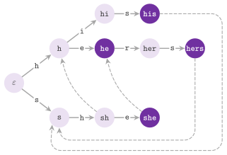
Lemma 15.9. After the automaton has read \(T[ 0 .. j ]\), its state is the longest suffix of \(T[ 0 .. j ]\) that is a prefix of some pattern, and the patterns that end at \(j\) are the suffixes of that state that are patterns. Also, for a state \(u c\), \(\mathit{fail}( u c ) = \delta( \mathit{fail}( u ) , c )\) (\(\varepsilon\) when \(u = \varepsilon\)).
Proof. By induction on \(j\). If \(u\) is the state after \(T[ 0 .. j - 1 ]\), every suffix of \(T[ 0 .. j ]\) that is a prefix of a pattern is \(x c\) with \(c = T[ j ]\) and \(x\) a suffix of \(u\) in the trie (by the hypothesis on \(u\)), and the chain \(u , \mathit{fail}( u ) , \ldots\) lists those suffixes by decreasing length; by (15.5), \(\delta( u , c )\) takes the first of them that goes on with \(c\). A pattern that ends at \(j\) is a suffix of \(T[ 0 .. j ]\) and a prefix of a pattern, hence a suffix of the state. The same argument shows that \(\delta( v , c )\) is the longest suffix of \(v c\) in the trie, for each state \(v\). A proper suffix of \(u c\) in the trie is \(\varepsilon\) or \(x c\), with \(x\) a proper suffix of \(u\) in the trie (the trie is closed under prefixes), and such an \(x\) is a suffix of \(\mathit{fail}( u )\); conversely each suffix of \(\mathit{fail}( u ) c\) is a proper suffix of \(u c\). Hence the longest proper suffix of \(u c\) in the trie is the longest suffix of \(\mathit{fail}( u ) c\) in it, i.e., \(\delta( \mathit{fail}( u ) , c )\). \(\square\)
We compute the failures in breadth-first order from \(\mathit{fail}( u c ) = \delta( \mathit{fail}( u ) , c )\), which only needs the transitions of a shallower state, and the same visit fills the missing transitions by (15.5) and the output link of each state, i.e., the nearest proper suffix of the state that is a whole pattern (Algorithm 15.4). Then the scan reports the patterns of the state and of the chain of its output links, at \(O( 1 )\) each:
Algorithm 15.4. The construction of the automaton of Aho and Corasick 1975 (Gusfield 1997, §3.4) and its search.
Theorem 15.2. The automaton of \(k\) patterns of \(M\) bytes takes \(O( 256 \, M )\) time and space to build, and it finds all the \(\mathit{occ}\) occurrences of the patterns in a text of \(n\) bytes in \(O( n + \mathit{occ} )\) time.
Proof. The trie has at most \(M + 1\) states, and the breadth-first visit spends \(O( 256 )\) on each. A byte of the text costs one transition. Also, each state visited on a chain of output links ends a pattern, which is reported (an empty pattern, the only one that the root would end, is not allowed). \(\square\)
findAll() gives the pairs (start, number) of the occurrences by
increasing end, the longer pattern first for one end; equal patterns get
one number each, in the order of add(). In the code, a state \(u\) with no
pattern of its own starts its chain at \(\mathit{out}( u )\), and the state
0 (the root) ends the chain. We use the same scan in count(), which only
counts, and forEach(), which hands each occurrence to a function of the
caller instead of storing it. A pattern added by add() after the
construction makes the automaton be built again, from the trie, by the
next call of build(); size() gives the number of patterns and
states() that of the states, at most \(M + 1\). The class is
// declarations of <ADS/string/AhoCorasick.h>
class AhoCorasick
{
 public:
 AhoCorasick( void );
 explicit AhoCorasick( const std::vector< std::string > & P );
 std::size_t add( std::string_view P );
 void build( void );
 [[nodiscard]] std::vector< std::pair< std::size_t , std::size_t > >
 findAll( std::string_view T ) const;
 [[nodiscard]] std::size_t count( std::string_view T ) const;
 template< class F >
 void forEach( std::string_view T , F && report ) const;
 [[nodiscard]] std::size_t size( void ) const;
 [[nodiscard]] std::size_t states( void ) const;
 };
and, for instance, with the header ADS/string/AhoCorasick.h, the
automaton of Figure 15.2 gives
ADS::AhoCorasick A( { "he" , "she" , "his" , "hers" } );
auto O = A.findAll( "ushers" );       // ( 1 , 1 ) for she, ( 2 , 0 )
                                      // for he, ( 2 , 3 ) for hers
std::size_t c = A.count( "ushers" );  // c is 3
15.3.2 The engineered search of many patterns¶
MultiSearcher of MultiSearch.h is the engineered search of many
patterns, on the filters of the FDR matcher of Hyperscan (Wang et al.
2019). One pattern goes to
StringSearcher; up to kFilter \(= 64\) patterns go through a filter of
shuffles of bytes, and more through a filter of shift-or on super
characters (filtered() is true for the first of the two). The
automaton of §15.3.1, built with the filter,
takes over where a filter lets too much through. A filter only proposes
candidate places, which are then checked against the patterns; we first
describe the two filters, then the switch to the automaton, and last the
count. findAll() gives the occurrences by increasing start and, for one
start, by increasing number. Since a filter finds the patterns of a place
bucket by bucket, and the automaton by end, the pairs are sorted at the
end. We forbid the empty pattern, and we call \(\ell\) the length of
the shortest pattern and \(\ell_{\max}\) that of the longest.
Buckets. The patterns, sorted in the lexicographic order, are cut into 8 buckets of \(\lceil k / 8 \rceil\) consecutive ones (the last buckets may be shorter or empty). The patterns of a bucket thus tend to share their first bytes, and the tables of a bucket may then admit few bytes that none of its patterns has. We tell the buckets apart by the 8 bits of a byte, which is the reason for their number.
The filter of shuffles. The place \(i\) of \(T\) is a candidate for the bucket \(b\) if the bit \(b\) of
is set. Here the tables \(\mathit{lo}_r\) and \(\mathit{hi}_r\) (16 bytes each) have the bit \(b\) set for the low and the high halves (4 bits) of the bytes \(r\) of the patterns of \(b\), for \(r < \min( 8 , \ell )\). A place thus passes for \(b\) when, for each \(r < q\), some pattern of \(b\) has its low half at \(r\) and some pattern of \(b\), maybe another, its high half. We take as \(q\), the number of bytes read, the least one, at most \(\min( 8 , \ell )\), for which a place passes with probability below \(2^{-10}\), the bytes of the text being drawn with the frequencies \(f( x )\) of the bytes in the patterns. By the union bound over the buckets, that probability is at most
which is computed for \(q = 1 , 2 , \ldots\) until it falls below
\(2^{-10}\); a large alphabet thus usually needs one or two bytes, and a
small one more. A table of 16 bytes is one register, and one lookup of
bytes in it (TableLookupBytes() of Highway, which is vpshufb on x86-64
and tbl on ARM) takes 16 places of \(T\) at once, or 32 in a vector of 32
bytes, with the table repeated in each half. A block of 32 places thus
costs \(q\) loads, \(2 q\) lookups per vector and a few logical operations,
with no branch but the one taken when some place of the block passes; the
places from \(n - \ell + 1\) on are masked off, and without Highway the
places are looked up one at a time in the same tables. A candidate is
checked against the patterns of its buckets: their first 8 bytes in one
comparison of words under a mask (for the patterns shorter than 8 bytes),
then the rest by memcmp().
The filter of shift-or. Above 64 patterns the halves of the bytes of a bucket cover nearly all the values, and the filter of shift-or of FDR takes over, on the first \(L = \min( 8 , \ell )\) bytes of the patterns. The super character \(x( p )\) of the place \(p\) is \(T[ p ]\) with the low 3 bits of \(T[ p + 1 ]\), 11 bits in all. Its mask \(\mathit{sh}[ x ]\) of 64 bits has the bit \(b\) of its byte \(L - 1 - r\) off (0) if a pattern of the bucket \(b\) has the super character \(x\) at its place \(r < L\), i.e., its byte \(r\) and the low bits of its byte \(r + 1\) (any 3 bits, when the pattern ends at \(r\)). The other bits of the bytes \(0 , \ldots , L - 1\) are on, while the bytes from \(L\) on are off, which makes them neutral for an OR. Now, a pattern of the bucket \(b\) that starts at \(s\) has, at its place \(p = s + r\), the bit \(b\) off in the byte \(L - 1 - r = e - p\) of \(\mathit{sh}[ x( p ) ]\), where \(e = s + L - 1\) is the end of its window. Hence it can occur only if the state
has the bit \(b\) off. In the scan we keep the states of 16 consecutive ends in
one register of 16 bytes, the byte \(x\) for the end \(j + x\): the 8 ends of
the current block of places \(j , \ldots , j + 7\), and the 8 after them,
which the masks of the block reach. For \(d < 8\) the 11 bits of \(x( j + d )\)
are those from the bit \(8 ( d \bmod 4 )\) of the word of 8 bytes read at
\(j\) (for \(d < 4\)) or at \(j + 4\) (for \(d \ge 4\)), so that two loads give
the super characters of a block. Each mask is moved by \(d\) bytes, with no
carry between the bytes, and ORed into the register: one load, one shift
of bytes and one OR a place. In all, the table of the masks takes
\(2^{11} \times 8\) bytes, i.e., 16 KB, and before the first block the
states of the ends \(0 , \ldots , L - 2\), which end no window, are all on.
A byte of the current 8 with a bit off sends the start \(e - L + 1\) of its
end to a table of the prefixes of \(L\) bytes of the patterns. The table has
\(2^{\max( 4 , \lceil \log_2 ( 2 k + 1 ) \rceil )}\) chains, reached by the
multiplicative hash of the prefix (\(\lfloor 2^{64} / \phi \rfloor\), as in
§15.2.2), and the patterns of a chain come in
increasing number. Each pattern of the chain is compared on its prefix, one
word, and then on its rest by memcmp().
Stride of 2. When each pattern has 8 bytes or more, the filter takes only the masks of the even places, which halves the loads and the ORs (a stride of 2, as FDR does on long patterns). A window holds \(W = \min( 8 , \lfloor \ell / 2 \rfloor )\) even places, and each pattern enters the masks twice. At its even offsets \(o = 2 t\) it serves the occurrences that start at an even place (in 4 buckets, the bits 0 to 3), and at its odd offsets \(o = 2 t + 1\) those that start at an odd place (in 4 more buckets, the bits 4 to 7), with \(\lceil k / 4 \rceil\) consecutive patterns a bucket. In either case the bit of the pattern is off in the byte \(W - 1 - t\) of the mask of its super character at the offset \(o\). A block covers the 16 places \(j , \ldots , j + 15\), with \(j\) even. The 11 bits of the place \(j + 2 d\) are those from the bit \(16 ( d \bmod 4 )\) of the word read at \(j\) or at \(j + 8\), the byte \(x\) of the state is the even end \(j + 2 x\), and the byte \(t\) of the mask of the place \(p\) reaches the end \(p + 2 t\). Hence the bits 0 to 3 of the end \(e\) test the start \(e - 2 ( W - 1 )\), the bits 4 to 7 the start \(e - 2 ( W - 1 ) - 1\), and each start of \(T\) is tested at one even end, by one of the two halves of the byte. We keep the stride of 2 only if a window passes with probability below \(2^{-8}\), the super characters of the text being drawn with their frequencies \(g( x )\) in the patterns:
This bound is looser than that of (15.7), since the buckets hold twice the patterns; when it fails, the filter of stride 1 searches.
Lemma 15.10. Neither filter misses an occurrence: the place of each occurrence of \(P_j\) is a candidate for the bucket of \(P_j\) (in the filter of shuffles), or its start is sent to the table of the prefixes (in the filters of shift-or).
Proof. In the filter of shuffles, \(q \le \ell \le | P_j |\), and for \(r < q\) the byte \(T[ i + r ] = P_j[ r ]\) sets the bit of the bucket of \(P_j\) in both tables, whence in each term of (15.6). In the filter of stride 1, \(L \le | P_j |\), and for \(r < L\) the super character of the place \(s + r\) of \(T\) is that of \(P_j\) at \(r\). When \(P_j\) ends at \(r\), the mask was cleared for every value of the 3 bits that follow. Hence each term of (15.8) has the bit of the bucket off (the bytes from \(L\) on add nothing), and so has \(\mathit{St}_e\). In the filter of stride 2, an occurrence that starts at \(s\) has the even end \(e = s + 2 ( W - 1 ) + ( s \bmod 2 )\), and the places \(e - 2 t = s + o\) with \(o = 2 ( W - 1 - t ) + ( s \bmod 2 ) \le 2 W - 1 \le \ell - 1\). The pattern entered the masks at all these offsets, in the half of the byte of the parity of \(s\), and the argument of stride 1 applies. In all the filters the check compares the whole pattern, and the table of the prefixes holds each pattern under its prefix. \(\square\)
Algorithm 15.5. The construction of
MultiSearcher and its search, after the FDR matcher of Wang et al.
2019.
The switch to the automaton. Both filters may let through a candidate at
nearly every place, on patterns that occur everywhere or on a text whose bytes
the filter cannot tell apart (a small alphabet, against patterns that use all
of it), or on long patterns whose first bytes occur everywhere. Each search
therefore counts the bytes that it compares with the patterns, as
StringSearcher does (§15.2.2): a word of 8 bytes
for each pattern compared at a candidate (in the filter of shuffles) or for
each entry of the chains visited (in the filters of shift-or), and the bytes
past the word that memcmp() compares when the word agrees. When they exceed
\(16 s + 4096\) after the block that starts at \(s\) (except on the last block of
the filter of shuffles without vector instructions), the search stops and
returns the first place that it has not tested, which automatonFrom( T )
also gives (std::string_view::npos if the filter searches all of \(T\)). This
is the end of the block of shuffles (\(s + 32\) or \(s + 64\)), or the first start
whose end lies in the next block of shift-or, \(j + 9 - L\) for the stride 1 and
\(j + 15 - 2 ( W - 1 )\) for the stride 2. We then let the automaton go on from
that place \(f\): it scans \(T\) from \(\max( f - \ell_{\max} , 0 )\) and reports
only the occurrences that start at \(f\) or later, the earlier ones being the
filter's.
Lemma 15.11. MultiSearcher::findAll()
gives \(\mathrm{Occ}( P_j , T )\) for each \(j\). Before the switch the
filter compares at most \(16 n + 4096\) bytes plus those of its last block,
at most \(64 ( M + 8 k )\). Hence the search takes \(O( n + M +
\mathit{occ} \log \mathit{occ} )\) time in the worst case, the last term
for the final sort, after a construction of \(O( 256 M + k \log k \,
\ell_{\max} )\) time.
Proof. By Lemma 15.10 the filter reports every occurrence that starts before \(f\), and none that starts later, since it stops after testing all the starts before \(f\). The automaton reports, by Lemma 15.9, all the occurrences that lie in \(T[ \max( f - \ell_{\max} , 0 ) .. ]\), which include those that start at \(f\) or later, and of these it keeps exactly the latter. As for the time, the filter costs \(O( 1 )\) per place, a check costs \(O( 1 )\) per byte counted, the bytes are bounded as stated (a block tests 64 places at most, each against at most the \(k\) patterns), and the automaton costs \(O( n + \mathit{occ} )\) by Theorem 15.2. In the construction we sort the patterns, with \(O( k \log k )\) comparisons of at most \(\ell_{\max}\) bytes, fills the tables in \(O( M )\) time and builds the automaton in \(O( 256 M )\). \(\square\)
We remark that counting the checks instead of the bytes would not make the
search linear, since a check may compare up to \(\ell_{\max}\) bytes. For
instance, the patterns \(a^{999} b\) and \(\mathtt{zzzzzzzz}\) on the text
\(a^n\) make every place a candidate of one check, and each check compares
about 1000 bytes; counted in bytes, the checks of the first block already
exceed the threshold, and the automaton searches the rest of the text (the
test engineered_strings.multi-search-worst).
The count. count() counts the occurrences of the filter and, after a
switch at the place \(f\), adds those of the automaton that start at \(f\) or
later, without listing them. With \(b = \max( f - \ell_{\max} , 0 )\), it
takes the count of the automaton on \(T[ b .. ]\) and subtracts the
occurrences that start before \(f\), which it lists on the window
\(T[ b .. f + \ell_{\max} )\) only. We remark that the subtraction is exact: an
occurrence that starts in \([ b , f )\) has at most \(\ell_{\max}\) symbols,
and thus lies in the window, while those that start before \(b\) are not
counted on \(T[ b .. ]\). The window costs \(O( \ell_{\max} )\) time besides
its occurrences. The class is
// declarations of <ADS/string/MultiSearch.h>
class MultiSearcher
{
 public:
 explicit MultiSearcher( const std::vector< std::string > & P );
 [[nodiscard]] std::vector< std::pair< std::size_t , std::size_t > >
 findAll( std::string_view T ) const;
 [[nodiscard]] std::size_t count( std::string_view T ) const;
 [[nodiscard]] std::size_t automatonFrom( std::string_view T ) const;
 [[nodiscard]] std::size_t size( void ) const;
 [[nodiscard]] bool filtered( void ) const;
 static constexpr std::size_t kFilter = 64;
 };
which one uses as AhoCorasick above, with the occurrences by start.
15.4 Edit distance, alignments and subsequences¶
In this section we compare two strings, \(P\) of \(m\) symbols and \(T\) of \(n\), by a table on their prefixes, as chapter 13 of Montresor 2025 does; the engineered algorithms of §15.4.5 compute the same values on words of 64 bits.
15.4.1 The approximate matching and the edit distance¶
An occurrence of \(P\) in \(T\) with \(k\) errors is a substring of \(T\) at edit distance \(k\) from \(P\), where an error is a substitution, an insertion (a symbol of \(P\) that is not in \(T\)) or a deletion (a symbol of \(T\) that is not in \(P\)). Let \(\mathit{DP}[ i ][ j ]\) be the least number of errors of an occurrence of the prefix \(P( i )\) that ends at the end of \(T( j )\) (Montresor 2025, §13.1, after Sellers 1980). Then
where \(\delta_{ij}\) is 0 if \(P[ i - 1 ] = T[ j - 1 ]\) and 1 otherwise; the edit distance of \(P\) and \(T\) is the same table with \(\mathit{DP}[ 0 ][ j ] = j\) in the first row, read at \(\mathit{DP}[ m ][ n ]\).
Lemma 15.12. The table (15.10) gives the least number of errors of an occurrence of \(P( i )\) ending at \(j\); with \(\mathit{DP}[ 0 ][ j ] = j\) it gives the edit distance of \(P( i )\) and \(T( j )\). Either table takes \(\Theta( m n )\) time.
Proof. Write an alignment of \(P( i )\) with a substring of \(T\) ending at \(j\) as a sequence of columns. Its last column aligns \(P[ i - 1 ]\) with \(T[ j - 1 ]\) (cost \(\delta_{ij}\)), or leaves \(P[ i - 1 ]\) out (an insertion, cost 1), or leaves \(T[ j - 1 ]\) out (a deletion, cost 1), and what precedes it is an alignment of the shorter prefixes, which in an optimal alignment is optimal itself. An occurrence may start anywhere, and the empty prefix of \(P\) costs 0 at every \(j\); in the edit distance the prefix \(T( j )\) must be used in full, and the empty prefix costs \(j\). \(\square\)
By the lemma, the best occurrences end where the last row is smallest
(stringMatching(), which returns the place \(j - 1\) of the last symbol of
the first such end \(j\), and its cost), and
occurrence() walks back from \(\mathit{DP}[ m ][ j ]\), following a term
that gave the minimum, to the place where the occurrence starts
(Montresor 2025, exercise 13.1).
Table 15.3 shows the table on a small example,
which matchingTable() fills row by row (Algorithm
15.6).
Table 15.3. The table (15.10) of
\(P = \texttt{aba}\) against \(T = \texttt{bacbab}\). The last row is smallest
(1 error) at \(j = 2\), \(j = 5\) and \(j = 6\), and stringMatching() returns
the first of them; from \(j = 2\), occurrence() goes back
through \(( 2 , 1 )\) and \(( 1 , 0 )\) to \(( 0 , 0 )\), i.e., the occurrence
\(\texttt{ba}\) with the first a of \(P\) left out.
| \(i \backslash j\) | 0 | 1 (b) |
2 (a) |
3 (c) |
4 (b) |
5 (a) |
6 (b) |
|---|---|---|---|---|---|---|---|
| 0 | 0 | 0 | 0 | 0 | 0 | 0 | 0 |
1 (a) |
1 | 1 | 0 | 1 | 1 | 0 | 1 |
2 (b) |
2 | 1 | 1 | 1 | 1 | 1 | 0 |
3 (a) |
3 | 2 | 1 | 2 | 2 | 1 | 1 |
Algorithm 15.6. The approximate matching of Montresor 2025, §13.1, the walk back to the start of an occurrence, and the version in two rows of §13.4.
Since a row of (15.10) depends only on the row above,
stringMatchingSingleRow() keeps two rows, \(O( n )\) space, and gives the
best cost alone (Montresor 2025, §13.4).
editDistance() does the same on the edit distance, with the rows of the
length of the shorter string (\(O( \min( m , n ) )\) space): it gives the
value, and no alignment.
We declare these functions, on any sequence S with size() and [], as
// declarations of <ADS/string/ApproximateMatching.h>
using Table = std::vector< std::vector< int > >;
template< class S >
Table matchingTable( const S & P , const S & T , bool edit = false );
template< class S >
std::pair< long , int > stringMatching( const S & P , const S & T );
template< class S >
std::size_t occurrence( const Table & DP , const S & P , const S & T ,
                        std::size_t j );
template< class S >
int stringMatchingSingleRow( const S & P , const S & T );
template< class S >
int editDistance( const S & P , const S & T );
where stringMatching() returns the place of the last symbol and the
cost, and occurrence() the start of the occurrence that ends at the
column \(j\) of the table, i.e., before \(T[ j ]\). For instance,
with the header ADS/string/ApproximateMatching.h, the example of Table
15.3 is
std::string P = "aba" , T = "bacbab";
auto [ e , k ] = ADS::stringMatching( P , T );  // e is 1, k is 1
ADS::Table DP = ADS::matchingTable( P , T );
std::size_t s = ADS::occurrence( DP , P , T , std::size_t( e + 1 ) );
// s is 0: the occurrence "ba"
int d = ADS::editDistance( P , T );  // d is 3
15.4.2 The longest common subsequence¶
We next consider the longest common subsequence (LCS) of \(P\) and \(T\)
(LongestCommonSubsequence.h, the reality check of Montresor 2025,
§13.7) has the same structure with a
maximum:
Lemma 15.13. \(\mathit{DP}[ i ][ j ]\) of (15.11) is the length of a longest common subsequence of \(P( i )\) and \(T( j )\).
Proof. If \(P[ i - 1 ] = T[ j - 1 ]\), some longest common subsequence ends with that symbol matched to both: one that does not use both last symbols can be changed, by an exchange, into one that does, of the same length. Otherwise a common subsequence leaves out \(P[ i - 1 ]\) or \(T[ j - 1 ]\). In both cases what remains is a common subsequence of the shorter prefixes. \(\square\)
lcsTable() fills (15.11) in \(\Theta( m n )\) time, and lcs() reads a
solution back from the last entry in \(O( m + n )\) steps, taking an equal
pair of symbols whenever it meets one; lcsMemo() is the memoized version
of the book, which solves only the subproblems it reaches:
diff() reads the differences of two sequences from the same table, as
the Unix command does on the lines of two files (Montresor 2025,
exercise 13.10; Hunt and McIlroy
1976): the items of \(P\) only are marked
'-', those of \(T\) only '+', and the common ones ' '. The longest
common substring (contiguous) has instead
\(\mathit{DP}[ i ][ j ] = \mathit{DP}[ i - 1 ][ j - 1 ] + 1\) if
\(P[ i - 1 ] = T[ j - 1 ]\) and 0 otherwise, its length being the largest
entry (Montresor 2025, exercise 13.2);
§15.5.5 solves it in linear time on a suffix
array.
We declare them as
// declarations of <ADS/string/LongestCommonSubsequence.h>
template< class S >
std::vector< std::vector< int > > lcsTable( const S & P , const S & T );
template< class S >
int lcsMemo( const S & P , const S & T , long * solved = nullptr );
template< class S >
S lcs( const S & P , const S & T );
template< class S >
std::vector< std::pair< char , typename S::value_type > > diff( const S & P ,
                                                               const S & T );
template< class S >
std::tuple< std::size_t , std::size_t , std::size_t >
longestCommonSubstring( const S & P , const S & T );
where longestCommonSubstring() gives the length and the starts in \(P\) and
in \(T\).
15.4.3 The alignments¶
An alignment of \(P\) and \(T\) (Alignment.h, Montresor 2025, exercises
13.7 to 13.9) inserts spaces in
either string, never one in front of the other, and each column scores
\(+1\) if the symbols are equal, \(-1\) if they differ and \(-2\) if one is a
space. Here the best score of the prefixes \(P( i )\) and \(T( j )\) is the maximum
of \(\mathit{DP}[ i ][ j - 1 ] - 2\), \(\mathit{DP}[ i - 1 ][ j ] - 2\) and
\(\mathit{DP}[ i - 1 ][ j - 1 ] + \delta_{ij}\), with \(\delta_{ij} = \pm 1\),
by the argument of Lemma 15.12. Also, the three kinds
differ only at the borders and in where the score is read: the global
alignment of Needleman and Wunsch 1970
has the borders \(-2 i\) and \(-2 j\) and its score in
\(\mathit{DP}[ m ][ n ]\). The semiglobal one has the borders 0 (the
spaces before the start and after the end of either string are free) and
its score is the best of the last row and column. Finally, the local one of
Smith and Waterman 1981, the best
alignment of two substrings, has 0 as a fourth term of the maximum and its
score in the best entry. Each takes \(\Theta( m n )\) time, and
globalAlignment() reads the two aligned strings back from the table.
The declarations are
// declarations of <ADS/string/Alignment.h>
enum class Alignment { GLOBAL , SEMIGLOBAL , LOCAL };
template< class S >
int alignmentScore( const S & P , const S & T , Alignment kind );
template< class S >
std::pair< S , S > globalAlignment( const S & P , const S & T ,
                                   typename S::value_type gap = ' ' );
15.4.4 Problems related to the subsequences¶
SubsequenceProblems.h solves four relatives of the LCS on sequences \(X\),
\(Y\), \(Z\) of lengths \(n\), \(m\), \(l\), each by a table on the prefixes. Whether
\(Z\) is a shuffle (an interleaving) of \(X\) and \(Y\) (isInterleaving())
is decided by \(D[ i ][ j ]\), true when \(Z[ 0 .. i + j )\) interleaves
\(X[ 0 .. i )\) and \(Y[ 0 .. j )\): it holds if \(D[ i - 1 ][ j ]\) does and
\(X[ i - 1 ] = Z[ i + j - 1 ]\), or if \(D[ i ][ j - 1 ]\) does and
\(Y[ j - 1 ] = Z[ i + j - 1 ]\), in \(\Theta( n m )\) time and one row of
space. A shortest common supersequence of \(X\) and \(Y\)
(shortestCommonSupersequence()) writes the items of a longest common
subsequence once and the others in their order.
Lemma 15.14. The shortest common supersequence of \(X\) and \(Y\) has length \(n + m - | \mathrm{LCS}( X , Y ) |\).
Proof. In a common supersequence \(W\), the items to which both an item of \(X\) and an item of \(Y\) are mapped form a common subsequence of \(X\) and \(Y\), and each other item of \(W\) serves one of the two; hence \(| W | \ge n + m - | \mathrm{LCS}( X , Y ) |\). Conversely, the supersequence read back from the table of the LCS attains the bound. \(\square\)
scsLength() gives only this length, from one row of the table of the
LCS, i.e., in \(\Theta( n m )\) time and \(O( m )\) space.
Lemma 15.15. The recurrence of \(D\) decides whether \(Z[ 0 .. i + j )\) is an interleaving of \(X[ 0 .. i )\) and \(Y[ 0 .. j )\), and \(C[ i ][ j ]\) of the recurrence below counts the occurrences of \(P( j )\) as a subsequence of \(T( i )\).
Proof. In an interleaving the last item of \(Z[ 0 .. i + j )\) comes from \(X\) or from \(Y\), and then it equals \(X[ i - 1 ]\) or \(Y[ j - 1 ]\), and the rest interleaves the shorter prefixes; conversely, an interleaving of the shorter prefixes followed by that item is one of the longer. The occurrences of \(P( j )\) in \(T( i )\) either do not use the place \(i - 1\), and are those in \(T( i - 1 )\), or match it to \(P[ j - 1 ]\), which requires \(T[ i - 1 ] = P[ j - 1 ]\), and are then the occurrences of \(P( j - 1 )\) in \(T( i - 1 )\) extended by it; the two kinds are disjoint. \(\square\)
The number of occurrences of \(P\) as a subsequence of \(T\)
(subsequenceOccurrences()), i.e., of the tuples of places
\(j_1 < \cdots < j_m\) with \(T[ j_k ] = P[ k ]\), satisfies
\(C[ i ][ j ] = C[ i - 1 ][ j ] + [ T[ i - 1 ] = P[ j - 1 ] ] \,
C[ i - 1 ][ j - 1 ]\); it is kept in one row updated from the right, and
given modulo \(2^{64}\), since it grows as the binomial coefficient
\(\binom{n}{m}\). Finally, lcs3() computes a longest common subsequence of
three sequences on the table of (15.11) in three dimensions,
\(\Theta( n m l )\) time and space. Taking the LCS of two of them and then of the
third is not a solution, since the longest pairwise one may leave out the
items that the third shares. For an unbounded number of strings the LCS
and the shortest common supersequence are NP-hard (Maier
1978). So is the shuffle of an
unbounded number of strings (Mansfield 1983)
and the iterated shuffle of one (Warmuth and Haussler
1984).
Each function has a template on the sequences, with
requires std::is_class_v< S >, and an overload on std::string:
// declarations of <ADS/string/SubsequenceProblems.h>
template< class S >
 requires std::is_class_v< S >
[[nodiscard]] bool isInterleaving( const S & X , const S & Y , const S & Z );
template< class S >
 requires std::is_class_v< S >
[[nodiscard]] std::size_t scsLength( const S & X , const S & Y );
template< class S >
 requires std::is_class_v< S >
[[nodiscard]] S shortestCommonSupersequence( const S & X , const S & Y );
template< class S >
 requires std::is_class_v< S >
[[nodiscard]] std::uint64_t subsequenceOccurrences( const S & P ,
                                                    const S & T );
template< class S >
 requires std::is_class_v< S >
[[nodiscard]] S lcs3( const S & X , const S & Y , const S & Z );
15.4.5 The engineered edit distance¶
EditDistance.h computes the edit distance, the length of the LCS and
the approximate search of the previous sections with the bit vectors of
Myers 1999 and the diagonal transitions
of Landau and Vishkin 1989; the
functions of §15.4.1 and
§15.4.2 remain the reference. Both rest on two
properties of the table of the distances.
Lemma 15.16. In the table (15.10), with either first row, two adjacent entries in a row or in a column differ by \(-1\), 0 or \(+1\), and the entries never decrease along a diagonal:
Proof. An alignment of \(P( i - 1 )\) with (a suffix of) \(T( j )\) becomes one of \(P( i )\) by one more insertion, whence \(D[ i ][ j ] \le D[ i - 1 ][ j ] + 1\). Conversely, in an optimal alignment of \(P( i )\), the symbol \(P[ i - 1 ]\) is either inserted, and then dropping its column gives an alignment of \(P( i - 1 )\) that costs 1 less, or aligned with a symbol of \(T\), and then turning that column into a deletion of the symbol of \(T\) costs at most 1 more; hence \(D[ i - 1 ][ j ] \le D[ i ][ j ] + 1\). We bound the horizontal differences in the same way, on the symbol \(T[ j - 1 ]\), which is deleted or aligned with a symbol of \(P\), with either first row. For the second part, each term of the minimum in (15.10) is at least \(D[ i - 1 ][ j - 1 ]\), e.g., \(D[ i - 1 ][ j ] + 1 \ge D[ i - 1 ][ j - 1 ]\) by the first part. \(\square\)
Bit vectors of Myers. By the first part of (15.12), a column of the table is determined by its top entry and by its vertical differences, kept in two bit vectors: \(P_v\) has the bit \(i\) set where the difference is \(+1\), and \(M_v\) where it is \(-1\). With \(\mathit{Eq} = \mathit{Peq}[ T[ j - 1 ] ]\) the places of \(P\) that hold the symbol, and \(h_{\mathit{in}}\) the horizontal difference at the top of a block of 64 rows, the block moves to the next column by the following operations, in the formulation of Hyyrö 2003:
The carries of the one addition propagate the horizontal differences down the column, and the dozen operations have no branch.
A column thus costs \(O( \lceil m / 64 \rceil )\) operations on words, and the distance \(O( n \lceil m / 64 \rceil )\) time, against the \(\Theta( m n )\) of the table (Myers 1999). We keep the bits \(\mathit{Peq}\) in \(256 \lceil m / 64 \rceil\) words; up to 4 blocks they lie in the object, and only the words of the bytes of the two strings are cleared beyond; a pair of strings thus costs \(O( m + n )\) for them, not \(256 \lceil m / 64 \rceil\).
Diagonal transitions. By the second part of (15.12), the furthest row \(F_h( k )\) of the diagonal \(k = j - i\) that \(h\) edits reach determines the table: it is the row reached by sliding along the matches of the diagonal from the best of the three cells that one more edit reaches,
and the distance is the least \(d\) with \(F_d( n - m ) = m\) (the diagonal transitions of Landau and Vishkin 1989, the furthest reaching paths of Myers 1986, and the wavefronts of Marco-Sola et al. 2021). We compare 8 bytes at a time in the slides.
Lemma 15.17. The rounds \(h \le d\) of (15.14) compute the edit distance \(d\) in \(O( ( n + m ) d )\) time in the worst case and \(O( d )\) space; on random strings the expected time is \(O( n + d^2 )\).
Proof. Round \(h\) handles the \(O( h )\) diagonals \(-h \le k \le h\). On one diagonal the rows reached by successive rounds never decrease, and the slides of a diagonal cover at most its \(O( n + m )\) cells in all, and the \(O( d )\) diagonals cost \(O( ( n + m ) d )\); the space holds two rounds. On random strings a slide stops after \(O( 1 )\) symbols in expectation, and the \(O( d^2 )\) pairs (round, diagonal) cost \(O( d^2 )\), plus \(O( n )\) for the slide of the main diagonal (Myers 1986). \(\square\)
With a longest common extension in \(O( 1 )\) for each slide (§15.5.6) the bound becomes \(O( n + d^2 )\) in the worst case; the library uses the direct comparison instead, which is likely to be the faster one on the usual strings, whose slides are usually short.
Band of Ukkonen. A path of cost at most \(t\) crosses only the diagonals \(i - j \in [ -t , t - ( n - m ) ]\), since each step off the main diagonal costs 1 (Ukkonen 1985a). Hence, with \(t\) a guess of \(d\), the blocks of the band give the distance if it is at most \(t\), and we double the guess until it is.
Lemma 15.18. Let \(r_t\) be the least cost of a path of the table within the band of \(t\). Then \(r_t \ge d\), and \(r_t \le t\) implies \(r_t = d\); doubling \(t\) from \(t_0 \ge 64\) until \(r_t \le t\) computes \(O( n ( d / 64 + \log ( 2 + d / 64 ) ) )\) blocks.
Proof. A path within the band is a path of the table, and so \(r_t \ge d\). If \(d < r_t \le t\), an optimal path, of cost \(d \le t\), would lie within the band, and \(r_t \le d\); hence \(r_t = d\). We stop the guess at the latest when \(t \ge d\), i.e., below \(2 \max\{ d , t_0 \}\), after at most \(\log_2 ( 2 \max\{ d , t_0 \} / t_0 ) + 1\) rounds. A round of width \(t\) computes at most \(( 2 t + 1 ) / 64 + 2\) blocks per column, and the widths, doubling, add up to less than twice the last one; summing over the \(n\) columns gives the bound. The blocks left out by the bounds to the end are those that no path of cost at most \(t\) crosses, and they change neither \(r_t\) when \(r_t \le t\) nor the test. \(\square\) In the band, as in edlib (Šošić and Šikić 2017), only the blocks that may still lead to the end within \(t\) are computed: a cell \(( i , j )\) costs at least \(D[ i ][ j ] + | ( m - i ) - ( n - j ) |\) to the end, and a cell of a block at least the bottom of the block minus its distance from it; the first and the last block go when the least of these bounds exceeds \(t\).
Strategy of levenshtein(). This function strips the common prefix and
suffix, puts the shorter string, of \(m\) bytes, in the column, and chooses by
size (Algorithm 15.7). One word suffices when
\(m \le 64\), i.e., \(O( n )\) time. For \(m > 128\) the diagonal transitions run
first, up to \(d \le n / 48 + 128\) (where they cost about as much as the
blocks), and give up once the rows reached by \(h = 32 , 64 , 128 , \ldots\)
edits suggest a distance more than twice as large. Then the band, from the
guess of the diagonals and a quarter more, doubles until the distance is at
most its width; once the bands have computed a quarter of the
\(n \lceil m / 64 \rceil\) blocks of the table, or span half of the column, all
the blocks are computed instead, four columns at a time; indeed, the block \(b\)
of the column \(j + q\) needs only the block \(b - 1\) of the same column and the
block \(b\) of the column before, so that the blocks \(i - q\) of the columns
\(j + q\), \(q < 4\), are independent (the four lanes of the vectors of
Highway, two vectors of two lanes on SSE2 and NEON, and without Highway
four chains of operations that overlap in the processor).
levenshtein( a , b , k ) does the same with \(k\) fixed, and gives \(k + 1\) for
any larger distance.
Algorithm 15.7. The engineered edit distance, without and with a bound \(k\).
Approximate search. approximateMatches( T , P , k ) gives the ends \(j\)
of the substrings of \(T\) at edit distance at most \(k\) from \(P\), with their
distances, by the search of Myers 1999 on
the table with the first row 0. By the second part of (15.12), a cell of value
at most \(k\) has a cell of value at most \(k\) on its diagonal in the column
before. Hence the last row of value at most \(k\) goes down by at most one row
per column, and only the blocks down to the last one with a cell at most
\(k + 1\) at its bottom are computed (the cut-off of Ukkonen
1985b), \(O( n k / 64 )\) expected time on
random texts.
Bit-parallel LCS. lcsLength() is the LCS of Allison and Dix
1986 in the form of Crochemore et al.
2001: with \(V = 1^m\) at first and
\(M = \mathit{Peq}[ b[ j ] ]\) for each byte of the second string,
the addition carried between the blocks, and the length is the number of 0 among the \(m\) bits of \(V\), in \(O( n \lceil m / 64 \rceil )\) time after the common prefix and suffix are stripped. We summarize the computations of the section in Table 15.4, and declare them as
// declarations of <ADS/string/EditDistance.h>
[[nodiscard]] inline std::size_t levenshtein( std::string_view a ,
                                              std::string_view b );
[[nodiscard]] inline std::size_t
levenshtein( std::string_view a , std::string_view b , std::size_t k );
[[nodiscard]] inline std::size_t lcsLength( std::string_view a ,
                                            std::string_view b );
[[nodiscard]] inline std::vector< std::pair< std::size_t , std::size_t > >
approximateMatches( std::string_view T , std::string_view P , std::size_t k );
For instance, with the header ADS/string/EditDistance.h,
std::size_t d = ADS::levenshtein( "kitten" , "sitting" );     // d is 3
std::size_t e = ADS::levenshtein( "kitten" , "sitting" , 2 );  // e is 3,
// the bound 2 exceeded
std::size_t l = ADS::lcsLength( "kitten" , "sitting" );  // l is 4
auto A = ADS::approximateMatches( "the cat sat" , "cot" , 1 );
// A is ( ( 7 , 1 ) ): "cat",
// which ends before the place 7
Table 15.4. The computations of the edit distance and of the LCS.
| Function | Time | Space | Remarks |
|---|---|---|---|
editDistance() |
\(\Theta( m n )\) | \(O( \min( m , n ) )\) | two rows, the value |
stringMatching(), lcs() |
\(\Theta( m n )\) | \(\Theta( m n )\) | the table of the book, a solution read back |
stringMatchingSingleRow() |
\(\Theta( m n )\) | \(O( n )\) | two rows, the value |
levenshtein() |
\(O( n \lceil m / 64 \rceil )\); usually \(O( n d / 64 )\) | \(O( \lceil m / 64 \rceil )\) words plus \(\mathit{Peq}\) | the diagonals (15.14) for small \(d\), then the band of Ukkonen |
approximateMatches() |
\(O( n \lceil m / 64 \rceil )\); \(O( n k / 64 )\) expected | as above | the cut-off of Ukkonen |
lcsLength() |
\(O( n \lceil m / 64 \rceil )\) | as above | Allison and Dix |
15.5 Suffix arrays, trees and automata¶
The suffixes of \(T\) hold all its substrings as their prefixes, and in this section we build three indexes that sort them (the suffix array), merge their common prefixes (the suffix tree), or merge the substrings with the same ends (the suffix automaton), and a pattern is then searched in a time that depends on \(m\) rather than on \(n\) (Ferragina 2023, chapter 10; Gusfield 1997).
15.5.1 The suffix array¶
We call suffix array of \(T\) (SuffixArray.h) the permutation \(\mathit{SA}\)
of \(0 , \ldots , n - 1\) such that \(T[ \mathit{SA}[ r ] .. ]\) is the
\(r\)-th smallest suffix in the lexicographic order (Manber and Myers
1993; Gonnet, Baeza-Yates and Snider
1992). It takes \(n\) integers besides
\(T\), against the 10 to 20 \(n\) bytes of a suffix tree. No terminator is
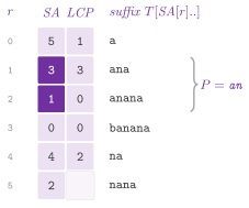
stored: Ferragina 2023 writes
\(T \$\), whose suffix \(\$\) would be the first of \(\mathit{SA}\)
(Figure 15.3). A text is a std::string_view,
whose symbols are its bytes, or a vector of integers in \([ 0 , K )\), e.g.,
several strings joined by distinct separators
(§15.5.5).
Lemma 15.19. The suffixes prefixed by \(P\) are consecutive in \(\mathit{SA}\): they are the suffixes not smaller than \(P\) and smaller than \(P \#\), where \(\#\) is a symbol larger than all the others.
Proof. A string is prefixed by \(P\) if and only if it lies between \(P\) and \(P \#\) in the lexicographic order. \(\square\)
Hence two binary searches give the range (range()), each step a
comparison of \(P\) with a suffix, in \(O( m \log n )\) time; the occurrences
are then listed in \(O( \mathit{occ} )\). By the search of Manber and Myers
1993 (rangeLcp()) we avoid comparing
the same symbols of \(P\) again. It keeps the lengths \(l\) and \(r\) of the
common prefixes of \(P\) with the suffixes at the two ends of the current
range. It also stores, for the middle \(M\) of each range that the binary search
may meet, the lcp of the suffix at \(M\) with the suffixes at the two ends
(\(\mathit{Llcp}[ M ]\) and \(\mathit{Rlcp}[ M ]\), \(2 n\) integers built from
\(\mathit{LCP}\) by build()). If, e.g., \(l \ge r\) and
\(\mathit{Llcp}[ M ] \ne l\), the side is decided with no comparison. If
\(\mathit{Llcp}[ M ] > l\), \(P\) compares with the suffix at \(M\) as with the
suffix at the left end, and if \(\mathit{Llcp}[ M ] < l\), \(P\) is smaller;
otherwise the comparison starts from the place \(l\)
(Algorithm 15.8).
Lemma 15.20. rangeLcp() finds the
range of \(P\) with \(O( m + \log n )\) comparisons of symbols.
Proof. Note that \(\max( l , r )\) never decreases: a step decided by \(\mathit{Llcp}\) or \(\mathit{Rlcp}\) keeps it, and a step that compares starts from it, and ends with the new lcp of \(P\) with one end. Each equal symbol compared increases it, which happens at most \(m\) times, and each step has at most one unequal comparison, over \(O( \log n )\) steps. \(\square\)
Algorithm 15.8. The two searches of a pattern in a suffix array: the plain binary search, and that of Manber and Myers 1993 on the arrays \(\mathit{Llcp}\) and \(\mathit{Rlcp}\).
We build the class SuffixArray on the bytes of a std::string_view,
which toSymbols() turns into the vector of integers Symbols, or on
such a vector with its alphabet \([ 0 , K )\); in both cases \(\mathit{SA}\)
comes from suffixArraySais() and \(\mathit{LCP}\) from lcpArray(). It
keeps the text (text()), \(\mathit{SA}\) (operator[], and the iterators
of a constant random-access range of its entries, with the member types
of a container), its inverse (rank(), built by inversePermutation()),
\(\mathit{LCP}\) (lcp()), the arrays \(\mathit{Llcp}\) and \(\mathit{Rlcp}\),
and the range minima of \(\mathit{LCP}\); count() and locate() take the
range of rangeLcp(), and the second gives the places in the order of
\(\mathit{SA}\). The functions of the namespace that build \(\mathit{SA}\)
and \(\mathit{LCP}\) by themselves, which we describe below, take either the bytes or
Symbols.
LCP array. The array \(\mathit{LCP}\) is computed in linear time by
the algorithm of Kasai et al. 2001
(lcpArray()), which rests on the following property.
Lemma 15.21. Let \(\mathit{PLCP}[ i ]\) be the lcp of the suffix \(i\) with the suffix before it in \(\mathit{SA}\) (0 for the first). Then
Proof. Let the suffix \(k\) precede the suffix \(i\) and share \(h > 0\) symbols with it. Then the suffix \(k + 1\) is smaller than the suffix \(i + 1\) and shares \(h - 1\) symbols with it, and so does every suffix between them in \(\mathit{SA}\), the one just before \(i + 1\) included. \(\square\)
Computing the lcp of the suffixes in the order of the text, each from the value of the previous one less one, therefore decreases \(h\) at most \(n\) times. Since \(h \le n\), there are at most \(2 n\) comparisons of symbols:
We compute the longest common extension of two suffixes, \(\mathrm{lce}( i , j )\),
as the minimum of \(\mathit{LCP}\) between their ranks, a query of range
minimum (chapter 6) in \(O( 1 )\) time after \(O( n )\) preprocessing
(lce()):
Constructions. The six constructions of SuffixArray.h give the
same array and differ in how they reuse the order of shorter strings
(Puglisi, Smyth and Turpin 2007).
suffixArraySorting() sorts the \(n\) suffixes by a sort of comparisons,
each comparison as long as the common prefix: \(O( n^2 \log n )\) time on a
text of one repeated symbol, and near \(O( n \log^2 n )\) on random texts.
By the prefix doubling of Manber and Myers 1993
(suffixArrayDoubling()) we give each suffix, after round \(k\), the rank of
its prefix of \(2^k\) symbols. We note that the pair of the ranks of the suffixes at \(i\)
and at \(i + 2^k\) is the rank of the prefix of \(2^{k+1}\) symbols, and the
pairs, made one key of 64 bits, are sorted by the LSD radix sort of
chapter 12 (which requires \(n < 2^{32}\)); hence \(O( n )\) per round, and
\(O( n \log n )\) in all, or \(O( n \log L )\) for \(L\) the length of the
longest repeated substring, since the ranks are all distinct after
\(\lceil \log_2 ( L + 1 ) \rceil\) rounds:
Furthermore, the doubling of Larsson and Sadakane 2007
(suffixArrayLarssonSadakane(), qsufsort) sorts in a round only the
groups of suffixes that are still tied, each by the rank of the suffix \(h\)
places ahead, and refines the ranks at once, and the groups already
sorted are skipped by a length stored in their first place. Its bound is
\(O( n \log n )\) with a ternary-split quicksort; with the sort of the
library inside the groups it is \(O( n \log^2 n )\) in the worst case, and
often close to linear on the usual texts.
Also, the Skew (DC3) algorithm of Kärkkäinen, Sanders and Burkhardt
2006 (suffixArraySkew()) names
the suffixes at the places \(i \bmod 3 \ne 0\) by the ranks of their
triples of symbols, sorted by three passes of radix sort, and sorts them
by the recursive suffix array of the string of the names, of \(2 n / 3\)
symbols, unless all the names differ. Then the suffixes at \(i \bmod 3 = 0\) are
sorted by the pair \(( T[ i ] , \mathrm{rank}( i + 1 ) )\), and the two lists
are merged by comparing a pair or a triple whose last item is a rank of the
sample. Hence
on an integer alphabet of \(O( n )\) symbols. Since the algorithm reduces the problem to sorting, it takes the optimal number of transfers of sorting on disk (chapter 23).
The induced sorting of Nong, Zhang and Chan 2011
(SA-IS, suffixArraySais()) classifies the suffixes as smaller or larger
than the next one: the suffix \(i\) is of type S if
\(T[ i .. ] < T[ i + 1 .. ]\), i.e., if \(T[ i ] < T[ i + 1 ]\), or
\(T[ i ] = T[ i + 1 ]\) and the suffix \(i + 1\) is of type S, and of type L
otherwise. It is an LMS place (leftmost S) if it is of type S and the
suffix \(i - 1\) of type L; Table 15.5 shows the
types of a classical example.
Table 15.5. The types of the suffixes of \(\texttt{mississippi\$}\); the LMS places (marked \(\ast\)) are 1, 4, 7 and 11, and the suffix array is \(11 , 10 , 7 , 4 , 1 , 0 , 9 , 8 , 6 , 3 , 5 , 2\).
| \(i\) | 0 | 1 | 2 | 3 | 4 | 5 | 6 | 7 | 8 | 9 | 10 | 11 |
|---|---|---|---|---|---|---|---|---|---|---|---|---|
| \(T[ i ]\) | m |
i |
s |
s |
i |
s |
s |
i |
p |
p |
i |
$ |
| type | L | S | L | L | S | L | L | S | L | L | L | S |
| LMS | \(\ast\) | \(\ast\) | \(\ast\) | \(\ast\) |
Lemma 15.22. Let the LMS-suffixes be placed, in their sorted order, at the ends of the buckets of their first symbols. Then a scan of \(\mathit{SA}\) from left to right that puts each suffix \(i - 1\) of type L at the head of its bucket, after it meets the suffix \(i\), followed by a scan from right to left that puts each suffix \(i - 1\) of type S at the tail of its bucket, sorts all the suffixes.
Proof. Within the bucket of a symbol \(c\) the suffixes of type L come before those of type S, since the first are followed by a run of \(c\) and then by a smaller symbol, the second by a larger one. Two suffixes \(i - 1\) and \(j - 1\) of type L in the same bucket compare as the suffixes \(i\) and \(j\), each of which is smaller than the suffix before it; by induction on the scan, the first scan meets \(i\) and \(j\) in their order before it places \(i - 1\) and \(j - 1\). Similarly, the second scan does the same for the type S, from the largest suffixes down, and it overwrites the LMS-suffixes placed at the start with their correct places. \(\square\)
The LMS-substrings (from an LMS place to the next one) are sorted by the same two scans, started from the LMS places in any order, as Nong, Zhang and Chan 2011 prove. If two of them are equal, their names, in the order of the text, form a string of at most \(n / 2\) symbols (two LMS places are never adjacent) whose suffix array, computed recursively, orders the LMS-suffixes; a last induction then sorts all the suffixes (Algorithm 15.9). Hence
with the smallest working space of the linear algorithms. We perform the induction by the procedure induce of Algorithm 15.9.
Algorithm 15.9. The induced sorting (SA-IS) of Nong, Zhang and Chan 2011, on a string whose last symbol is a unique 0.
Finally, suffixArrayScan() is the algorithm of Gonnet, Baeza-Yates and
Snider 1992 for the disk. In it, the text is
cut into blocks of \(b\) symbols, scanned from left to right; the suffixes
that start in a block are sorted by comparisons, each earlier suffix is
placed among them by binary search, and the counts of the earlier suffixes
that fall between two consecutive suffixes of the block merge the two
arrays in one scan of the older one. It makes \(O( ( n^2 / b ) \log b )\)
comparisons of suffixes, i.e., cubic time in the worst case, but all its
passes are sequential, and on disk it thus reads and writes only by scans.
Table 15.6 summarizes the constructions.
Table 15.6. The constructions of the suffix array; \(L\) is the length of the longest repeated substring and \(b\) the length of a block.
| Function | Time | Remarks |
|---|---|---|
suffixArraySorting() |
\(O( n^2 \log n )\), near \(O( n \log^2 n )\) on random texts | a sort of comparisons, each as long as an lcp |
suffixArrayDoubling() |
\(O( n \log L ) \subseteq O( n \log n )\) | Manber and Myers, a radix sort of pairs of ranks per round |
suffixArrayLarssonSadakane() |
\(O( n \log^2 n )\) here | only the groups still tied are sorted |
suffixArraySkew() |
\(O( n )\) | (15.17); optimal transfers on disk |
suffixArraySais() |
\(O( n )\) | (15.18); engineered as suffixArray() of SuffixSorting.h (§15.5.2) |
suffixArrayScan() |
\(O( ( n^2 / b ) \log b )\) comparisons of suffixes | all its passes sequential |
Each construction has an overload on the bytes and one on Symbols (with
the alphabet \(K\) for Skew and SA-IS, and the block \(b\), named m in the
header, for the scan); we list those on the bytes and the class:
// declarations of <ADS/string/SuffixArray.h>
using Symbols = std::vector< std::size_t >;
[[nodiscard]] inline Symbols toSymbols( std::string_view T );
[[nodiscard]] inline std::vector< std::size_t >
suffixArraySorting( std::string_view T );
[[nodiscard]] inline std::vector< std::size_t >
suffixArrayDoubling( std::string_view T );
[[nodiscard]] inline std::vector< std::size_t >
suffixArrayLarssonSadakane( std::string_view T );
[[nodiscard]] inline std::vector< std::size_t >
suffixArraySkew( std::string_view T );
[[nodiscard]] inline std::vector< std::size_t >
suffixArraySais( std::string_view T );
[[nodiscard]] inline std::vector< std::size_t >
suffixArrayScan( std::string_view T , std::size_t m );
[[nodiscard]] inline std::vector< std::size_t >
inversePermutation( const std::vector< std::size_t > & SA );
[[nodiscard]] inline std::vector< std::size_t >
lcpArray( std::string_view T , const std::vector< std::size_t > & SA );

class SuffixArray
{
 public:
 SuffixArray( void ) = default;
 explicit SuffixArray( std::string_view T );
 SuffixArray( Symbols T , std::size_t K );
 [[nodiscard]] std::pair< std::size_t , std::size_t >
 range( std::string_view P , long * comparisons = nullptr ) const;
 [[nodiscard]] std::pair< std::size_t , std::size_t >
 rangeLcp( std::string_view P , long * comparisons = nullptr ) const;
 [[nodiscard]] std::size_t count( std::string_view P ) const;
 [[nodiscard]] std::vector< std::size_t > locate( std::string_view P ) const;
 [[nodiscard]] std::size_t lce( std::size_t i , std::size_t j ) const;
 [[nodiscard]] std::size_t rank( std::size_t i ) const;
 [[nodiscard]] std::size_t operator[]( std::size_t r ) const;
 [[nodiscard]] std::size_t size( void ) const;
 [[nodiscard]] const Symbols & text( void ) const;
 [[nodiscard]] const std::vector< std::size_t > & lcp( void ) const;
 };
where range() and rangeLcp() (also on Symbols) give the range
\([ \mathit{lo} , \mathit{hi} )\) of the ranks. For instance, with the header
ADS/string/SuffixArray.h, Figure 15.3 is
ADS::SuffixArray S( "banana" );        // SA is ( 5 , 3 , 1 , 0 , 4 , 2 )
auto [ lo , hi ] = S.rangeLcp( "an" );  // the ranks 1 and 2: lo is 1,
                                       // hi is 3
std::vector< std::size_t > L = S.locate( "an" );  // L is ( 3 , 1 )
std::size_t e = S.lce( 1 , 3 );                    // e is 3, "ana"
15.5.2 The engineered suffix sorting¶
suffixArray() of SuffixSorting.h is SA-IS on the integers I of 32
bits, or of 64 bits, which a text of \(2^{31} - 1\) symbols or more
requires. It takes the bytes of a std::string_view (\(K = 256\)), or a
vector of integers in \([ 0 , K )\) (the second overload, which lacks the
steps that need bytes). We build the array in the signed integers of the
same width, whose top bit the steps below use as a mark, and
lcpArrayPhi() is the engineered LCP array. A level of the recursion
takes \(T\), the \(n\) words of \(\mathit{SA}\), \(n / 32\) words for two bit
vectors (the types and the LMS places), and at most \(15 K\) words: the
counts of the kinds take \(4 K\), the sizes and the heads of the buckets
\(2 K\), the seeds \(K\) and the parts of the partial induction \(8 K\). The
levels together take \(O( n )\) words, since a level has at most half the
symbols of the one above. We describe the steps in the order in which
they run (Algorithm 15.10).
Types by the carries. The types are computed 64 places a word, from the last word to the first. In a word, let \(G\) have the bit of the place \(i\) set if \(T[ i ] < T[ i + 1 ]\), and \(E\) if \(T[ i ] = T[ i + 1 ]\). Both come from vector comparisons, with the bits reversed so that the higher places are the lower bits; the place \(n - 1\) has neither bit and is of type L, as if \(T[ n ]\) were smaller than every symbol.
Lemma 15.23. Let \(c\) be the type of the place that follows the word (1 for S, 0 for L, and 0 after the last word), and let \(X\) be the carries out of the bits of the sum \(G + ( G \vee E ) + c\) on 64 bits. Then the bit of \(X\) of the place \(i\) is 1 if and only if \(t_i = S\), and the carry out of the whole sum is the type of the first place of the word.
Proof. The carry out of a bit is \(\mathrm{maj}( a , a' , z )\), with \(a\) and \(a'\) the bits of \(G\) and of \(G \vee E\) there and \(z\) the carry in. If \(a = 1\) then \(a' = 1\), and the carry is 1; if \(a = 0\) then \(a' = E_i\), and the carry is \(E_i \wedge z\). Hence the carry out of the bit of \(i\) is \(G_i \vee ( E_i \wedge z )\), where \(z\) is the carry out of the bit of the place \(i + 1\) (the lower bit), or \(c\) for the last place of the word. This is the rule of the types: \(t_i = S\) if and only if \(T[ i ] < T[ i + 1 ]\), or \(T[ i ] = T[ i + 1 ]\) and \(t_{i+1} = S\). By induction on the places, from the higher to the lower, the carries are the types. \(\square\)
We read the carries from the sum \(s\) as \(( s \oplus G \oplus ( G \vee E ) ) \gg 1\), with the carry out of the top bit (that of either of the two additions) put back in the bit 63. A word thus costs a few operations, and only the carry passes from word to word. The suffixes \(i \ge 1\) then fall into four kinds by the types of \(i\) and \(i - 1\) (LL, LS, LMS and SS, the LMS places being those of type S after a place of type L). We count the kinds per first symbol with no branch: the counter \(4 T[ i ] + \mathit{kind}\) of each of 64 places is built by vector operations from the two words of the types. On bytes, or on alphabets of at most 1024 symbols, the counts go into two histograms, one for the even places and one for the odd, so that equal symbols in a row do not wait for each other's increments. Two LMS places are never adjacent; there are thus \(m \le \lfloor n / 2 \rfloor\) of them, kept in a bit vector.
No LMS place. If \(m = 0\), the places of type S, if any, form a prefix of \(T\). With none (the suffix 0 is of type L) the text never rises, each suffix is larger than the next, and \(\mathit{SA} = n - 1 , \ldots , 0\) at once. Otherwise one induction from the empty array, started as always from the suffix \(n - 1\), sorts all the suffixes.
Direct sort of the LMS-suffixes. On a text of bytes the LMS-suffixes are first sorted directly, as strings, and the induction only follows (the two stages of Itoh and Tanaka 1999 and of DivSufSort, Fischer and Kurpicz 2017, on the LMS-suffixes of SA-IS). We rank the \(\sigma\) bytes that occur. When \(\sigma \le 64\) the text is packed in codes of \(\beta = \lceil \log_2 \sigma \rceil\) bits, and otherwise the bytes themselves are used (\(\beta = 8\)); the window of 64 bits at the bit \(\beta p\) of the packed text thus holds the first \(\lfloor 64 / \beta \rfloor\) symbols of the suffix \(p\), with zeros past the end. We try the method only if a sample of about 1024 windows of 32 bits, taken at LMS places spread over the text, has at most one equal pair in 256. On a text with no long repeats two windows are equal with probability about \(2^{-32}\), whereas a few equal pairs reveal many ties, which the induction resolves in less time (as on English, or on long repeats). Each LMS place then gets an item, made of the top \(\kappa\) bits of its window and of the place: with \(\kappa = 32\) on 32 bits, in one word whose high half is the key, so that the items compare as their keys, and with \(\kappa = 64\) on 64 bits, in two words.
We sort the items by a radix sort on the top \(N = \min( \kappa , \lceil \log_2 ( m + 1 ) \rceil + 6 )\) bits of their keys. When \(m \ge 2^{16}\) they are first distributed into the 256 buckets of the top 8 bits (on bytes, by the counts of the LMS places of each first symbol, which the classification gives), which then fit in the cache; when \(m < 2^{16}\) all the items form one bucket. Each bucket goes on with its remaining bits, by at most 3 passes of at most \(\min( 11 , \lceil \log_2 ( g + 1 ) \rceil + 1 )\) bits for a bucket of \(g\) items, and a bucket of at most 16 items is sorted by insertion instead. Since \(N\) exceeds \(\log_2 m\) by six bits, on a text with no long repeats about \(m^2 / 2^{N+1} \le m / 128\) pairs of items remain equal on the \(N\) bits. These runs are sorted on their whole keys, by insertion if they have at most 16 items and by a sort of comparisons otherwise. The suffixes of equal keys go on to the windows at the bits \(\beta p + \kappa , \beta p + \kappa + 64 , \ldots\), and each group is sorted on the pair (window, bits left). A suffix that ends inside the window, i.e., with fewer than 64 bits of text left, thus comes before one that goes on with the same bits, the shorter first, and a group still equal with 64 bits left goes on to the next window. Note that this step reads the text in order, against the 2 random reads a suffix of the partial induction, and it needs no names and no recursion. It is given up for the partial induction once the ties have read more than \(m\) windows in all.
Partial induction and names. Otherwise the LMS-substrings (from an LMS place to the next one) are sorted by the two scans of Lemma 15.22, started from the LMS places in the order of the text. To this end, the array is split by the type of the suffix before each entry. An area A holds, for each symbol \(c\), an LL part (the L-suffixes after an L-suffix) and an LMS part (the seeds), i.e., the entries whose predecessor is of type L and is moved by the scan from left to right. An area C holds, for each \(c\), an LS part and an SS part, i.e., the entries whose predecessor is of type S and is moved by the scan from right to left. Each scan thus visits only one area, and no entry with nothing to do. First, the seeds are written by their first symbol, the first of each symbol marked. Then the scan of A moves each suffix \(p - 1\) of type L to the LL part of its symbol if \(p - 2\) is of type L, and to its LS part otherwise. Last, the scan of C, from right to left, moves each suffix \(p - 1\) of type S to the SS part of its symbol if \(p - 2\) is of type S, and otherwise among the sorted LMS places, which fill \(\mathit{SA}[ 0 .. m )\) per symbol from the end (A has been scanned by then, so that its place can be reused).
Both scans name the substrings as they go. A scan counts in \(d\) the marks of the entries it meets, so that \(d\) is the name of the current entry, and a moved suffix is marked, by the top bit of its entry, unless the last suffix moved into the same part came from an entry of the same name. Between the two scans the marks of the LS parts are moved one place to the left; a mark then means that an entry differs from the one after it, as the scan from right to left meets them. At the end the marks of \(\mathit{SA}[ 0 .. m )\) become the bit vector of the ends of the groups of equal LMS-substrings (read a vector of entries at a time with Highway), and their number is the number of names. In the code, the scans move two entries a step and prefetch the text of the entries 64 places ahead; beyond 65536 symbols they also prefetch the parts and the places these point to.
Ties. If two LMS-substrings are equal, the order of their suffixes depends on the text that follows them, and three methods are tried in turn, each usually cheaper than the next when it applies. First, on bytes, when the groups of equal names hold at most 16 suffixes on average, the text is read. Two LMS-suffixes \(p\) and \(p'\) of a group, whose LMS-substrings have the same length \(l\), are compared by \(T[ p + l .. ]\) and \(T[ p' + l .. ]\), read 8 bytes a round as one key in the order of the bytes; a suffix that ends inside the key comes before one that goes on with the same bytes. A group of at most 16 suffixes is sorted on its keys by insertion. A larger one is sorted by a radix sort, in passes of 8 bits, on the bits that are not the same in all its keys (gathered in their order, a run of 1s of their mask at a time, when they are at most 32 and no suffix ends inside the keys), or else by a sort of comparisons; the parts still tied go to the next round. The rounds are at most 8 and read at most \(2 m\) keys. Before them, a first round on the groups that hold the first eighth of the tied suffixes decides whether the method is worth its cost: if half of them stay tied (long repeats), the other rounds are skipped. We then write the names, in the slot \(m + \lfloor p / 2 \rfloor\) of each LMS place \(p\), as the ranks of the groups left; they are finer than the names of the LMS-substrings, since equal names still mean equal LMS-substrings and a smaller name a smaller suffix.
Second, if at most \(m / 4\) suffixes are still tied, each group is sorted by the names of the LMS places that follow its suffixes, compared one after the other until they differ (a suffix that runs out of LMS places comes first). The names compared are at most \(m\) in all, the suffixes of the other names are already in place, and no recursion is needed. Third, the names are gathered in \(R = \mathit{SA}[ m .. 2 m )\) in the order of the text, and the LMS-suffixes are sorted as the suffixes of \(R\). When at most \(m / 4\) suffixes are tied, or the tied groups have at most 16 suffixes on average, this is done by the doubling of Larsson and Sadakane 2007 restricted to the groups of equal names, and otherwise by the recursion \(\mathrm{suffixArray}( R )\) on the alphabet of the names. In turn, the doubling first sorts the suffixes by a counting sort on their names, so that a name that occurs once is in place at once. In the round \(h = 1 , 2 , 4 , \ldots\) a group of suffixes equal on their first \(h\) names is sorted by \(V[ i + h ]\), the rank of the suffix \(h\) places ahead (the last place of its group), by insertion up to 16 suffixes and by a sort of comparisons beyond, in \(O( g \log g )\) time for a group of \(g\). We give up the doubling for the recursion if more suffixes than its limit are still tied after a round, or once \(h\) exceeds \(2^{16}\), i.e., after 17 rounds. Finally, the ranks found are mapped back to the LMS places, listed in the order of the text by their bit vector.
Lemma 15.24. Each of the three methods gives the LMS-suffixes in their order. The names written after the first one satisfy the following: equal names imply equal LMS-substrings, and among the LMS-suffixes with different names a smaller name means a smaller suffix.
Proof. Two LMS-suffixes \(p\) and \(p'\) with equal LMS-substrings of length \(l\) compare as \(T[ p + l .. ]\) and \(T[ p' + l .. ]\). The keys of the first method compare these strings 8 bytes at a time, a string that ends first being the smaller; a group split by its keys is thus in its final order, and its new groups have equal LMS-substrings and are ranked as their suffixes. In the second method, \(T[ p + l .. ]\) starts at the next LMS place of \(p\). The suffix from an LMS place compares as the string of the names of the LMS places from it on, by the property of the names just stated applied at each LMS place, and a string of names that ends first is the smaller, since its suffix of \(T\) ends first. The third method sorts the same strings of names as the suffixes of \(R\), by the doubling or by the recursion. \(\square\)
Placement and induction. The sorted LMS places come grouped by their
first symbol, so that each group is moved at once by memmove() to the
end of its bucket, from the last symbol to the first, and the places in
between are cleared. Then the two scans of
Lemma 15.22 sort all the suffixes, the scan
from left to right being started by the suffix \(n - 1\) at the head of its
bucket. An entry is stored with its top bit set when the suffix before it
is of the other type, i.e., of type S for an L-suffix stored by the first
scan and of type L for an S-suffix stored by the second; the bit comes
from \(T[ p - 1 ]\) and \(T[ p ]\) by a shift and no branch. The scan from
left to right moves the entries without the bit (whose predecessor is of
type L) and flips the bit of each entry it passes. The scan from right to
left then finds without the bit exactly the entries whose predecessor is
of type S, moves them, and clears the bit of the others. The text before
the entries 64 places ahead is prefetched at a place chosen by a select,
with no branch on an empty entry; beyond 65536 symbols the heads of the
buckets and the places they point to are prefetched too.
Algorithm 15.10. The engineered SA-IS of
suffixArray(), for bytes and for integers.
Lemma 15.25. suffixArray() returns
the suffix array of \(T\) in \(O( ( n + K ) \log n )\) time in the worst case,
and in \(O( n + K )\) time when the radix sorts and the recursion settle the
order of the LMS-suffixes.
Proof. The order is correct by Lemma 15.22, whose hypothesis the three methods of Lemma 15.24 and the direct sort establish (the latter sorts the LMS-suffixes as strings, window after window). A level of the recursion makes the classification, the scans and the placement in \(O( n + K )\) time; the direct sort makes a radix sort of \(O( m )\) and is given up after \(O( m )\) windows of ties; the first two methods of the ties are bounded by their budgets of \(O( m )\) keys or names, and the doubling by its 17 rounds of \(O( m \log m )\) each. Hence a level costs \(O( n + K + m \log m )\), and \(O( n + K )\) when no sort of comparisons runs. The recursion gets at most \(\lfloor n / 2 \rfloor\) symbols, at most as many names, and the sum over the levels is geometric. \(\square\)
The contracts check the result as a suffix array, by an audit of \(O( n )\) time.
LCP array by \(\Phi\). lcpArrayPhi() is the algorithm of
Kärkkäinen, Manzini and Puglisi 2009:
with \(\Phi[ \mathit{SA}[ r ] ] = \mathit{SA}[ r - 1 ]\), the permuted LCP
\(\mathit{PLCP}[ i ] = \mathrm{lcp}( T[ i .. ] , T[ \Phi[ i ] .. ] )\) is
computed in the order of the text by (15.16), \(2 n\) comparisons of symbols
in all, with no access to the inverse of \(\mathit{SA}\); then
\(\mathit{LCP}[ r ] = \mathit{PLCP}[ \mathit{SA}[ r + 1 ] ]\) costs one
random read per entry, which falls into a copy of \(\mathit{PLCP}\) in \(n\)
bytes (capped at 255) when \(n\) integers no longer fit in the cache.
\(\Phi\) and \(\mathit{PLCP}\) share one array of \(n\) integers.
The declarations of SuffixSorting.h are
// declarations of <ADS/string/SuffixSorting.h>
template< class I = std::uint32_t >
 requires( std::same_as< I , std::uint32_t > ||
           std::same_as< I , std::uint64_t > )
[[nodiscard]] std::vector< I > suffixArray( std::string_view T );
template< class I >
 requires( std::same_as< I , std::uint32_t > ||
           std::same_as< I , std::uint64_t > )
[[nodiscard]] std::vector< I > suffixArray( const std::vector< I > & T ,
                                            std::size_t K );
template< class I >
[[nodiscard]] std::vector< I > plcpArray( std::string_view T ,
                                          const std::vector< I > & SA );
template< class I >
[[nodiscard]] std::vector< I > lcpArrayPhi( std::string_view T ,
                                            const std::vector< I > & SA );
and, e.g., ADS::suffixArray( T ) gives the array of
ADS::suffixArraySais( T ) in 32-bit integers.
15.5.3 The suffix tree¶
We call suffix tree of \(T\) (SuffixTree.h) the compact trie (chapter 7)
of the \(n + 1\) suffixes of \(T \$\), where the terminator makes each suffix
end in a leaf of its own (Figure 15.4). Each edge has as label
a substring of \(T\), kept as the place of one occurrence and
the string depths of its two ends, and the children of a node are kept by
their first symbol in a balanced search tree (std::map), whence
branching costs \(O( \log \sigma )\) and the children are visited in the
lexicographic order.
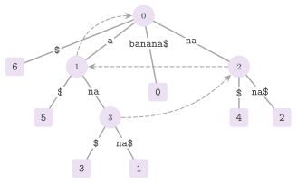
Lemma 15.26. The suffix tree of \(T\) has \(n + 1\) leaves and at most \(n\) internal nodes, and it takes \(O( n )\) space. A node \(u\) is internal if and only if the string \(s[ u ]\) that it spells occurs at least twice in \(T \$\) followed by distinct symbols, and the lowest common ancestor of the leaves \(i\) and \(j\) spells the longest common prefix of the suffixes \(i\) and \(j\).
Proof. Every internal node but the root has at least two children, and a tree with \(n + 1\) leaves and this property has at most \(n\) internal nodes; each edge takes \(O( 1 )\) space. A node branches exactly where two suffixes that share \(s[ u ]\) continue differently. Finally, the path from the root to the lowest common ancestor is the longest path shared by the two leaves, i.e., their longest common prefix. \(\square\)
The engineered suffix trees of the literature take some 10 to 20 \(n\) bytes
(Abouelhoda, Kurtz and Ohlebusch
2004). Ours keeps 5 words and a
std::map in each node, i.e., 88 bytes, and 48 more per child in the map
of libstdc++, about \(270 n\) bytes in all, which is why we treat the suffix
array first. All three constructions give the same tree.
Naive construction. Build::naive inserts the suffixes from the
longest one, each by a walk down from the root that compares all its
symbols: \(\Theta( n^2 )\) time on \(a^{n-1}\).
McCreight's construction. The algorithm of McCreight
1976 (Build::mcCreight) also
inserts the suffixes from the longest one. Let \(\mathit{head}_i\) be the
longest prefix of the suffix \(i\) that is a prefix of an earlier suffix,
i.e., the locus where the leaf of \(i\) is attached. Then
\(\mathit{head}_{i-1}\) without its first symbol is a prefix of
\(\mathit{head}_i\), since the earlier suffix that shares \(\mathit{head}_{i-1}\)
with the suffix \(i - 1\), shifted by one, shares it with the suffix \(i\).
Hence the walk of the suffix \(i\) starts from the node that spells
\(\mathit{head}_{i-1}\) without its first symbol, which the suffix link of
the node of \(\mathit{head}_{i-1}\) gives. When that link is not set yet, it
is found from the link of the parent by a rescan that compares only the
first symbol of each edge (the string is known to be in the tree), and
then a scan compares the symbols past it (the procedure mcCreight of the
pseudocode above).
Theorem 15.3. McCreight's construction takes \(O( n \log \sigma )\) time.
Proof. The scan compares the symbols of the suffix \(i\) past \(\mathit{head}_{i-1}\) without its first symbol, and ends at \(\mathit{head}_i\); since \(| \mathit{head}_i | \ge | \mathit{head}_{i-1} | - 1\), the scans compare \(O( n )\) symbols in all. A rescan jumps over whole edges, each jump increasing the node depth (the number of nodes on the path from the root) of the current node, while following a link decreases it by at most 2 (the parent and the link); since the node depth is at most \(n\), the jumps are \(O( n )\) in all. Each step branches at a node in \(O( \log \sigma )\). \(\square\)
Construction from the suffix array. Build::suffixArray builds
\(\mathit{SA}\) by SA-IS and \(\mathit{LCP}\) by Kasai et al., and inserts the
leaves in the order of \(\mathit{SA}\): the leaf of rank \(r\) climbs from the
previous leaf, along the rightmost path, to the deepest node of string
depth at most \(\mathit{LCP}[ r - 1 ]\), and splits the edge below it when
that depth is smaller (the procedure fromSuffixArray of the
same pseudocode).
Lemma 15.27. The construction from \(\mathit{SA}\) and \(\mathit{LCP}\) takes \(O( n )\) time besides the two arrays.
Proof. By construction, the tree is built in the lexicographic order of the leaves, so that the new leaf hangs from the rightmost path. Each edge climbed leaves the rightmost path for good, since the new leaf hangs to its right; each step thus climbs over an edge that is never climbed again, and the edges are \(O( n )\). \(\square\)
Weiner 1973 gave the first linear construction, inserting the suffixes from the shortest one; the online algorithm of Ukkonen 1995 is a left-to-right form of McCreight's; and Farach 1997 reached \(O( n )\) on integer alphabets by merging the trees of the odd and of the even suffixes, the idea that the Skew algorithm turned into the split \(2 / 3 : 1 / 3\). Since the linear suffix arrays are smaller and (usually) faster, the construction through \(\mathit{SA}\) and \(\mathit{LCP}\) is the usual one, whereas McCreight's may pay where the average lcp is small.
Queries. locus() finds the extended locus of \(P\) by a walk down
from the root in \(O( m \log \sigma )\), and locate() the \(\mathit{occ}\)
leaves below it in \(O( \mathit{occ} )\), since that subtree has
\(\mathit{occ}\) leaves and fewer internal nodes. lca() answers the lowest
common ancestor of two nodes in \(O( 1 )\) by the Euler tour of the tree
and the range minima of its depths (Bender and Farach-Colton
2000), and hence lce() gives the
longest common extension of two suffixes by
Lemma 15.26. toSuffixArray() reads
\(\mathit{SA}\) and \(\mathit{LCP}\) back by a visit in order: the leaves give
\(\mathit{SA}\), and the shallowest internal node met between two leaves
their lcp.
We keep the nodes in a vector, the root being root() \(= 0\), and each
is a Node with the place pos of one occurrence of its string, its
string depth depth, its parent, the suffix of a leaf (npos for
an internal node), the number of leaves below it and its children by
their first symbol. Also, node(), leaf() (the leaf of a suffix, the
terminator being the suffix \(n\)), symbol() (the symbols as stored,
those of \(T\) plus 1 and 0 for the terminator), textSize(), size()
(the number of nodes), count() (the leaves below the locus, the
terminator left out), preorder() (the nodes with the children by
increasing first symbol) and the iterators over the nodes complete the
interface; the enumeration Build chooses the construction, McCreight's
by default.
In all, the class is
// declarations of <ADS/string/SuffixTree.h>
class SuffixTree
{
 public:
 static constexpr std::size_t npos = std::numeric_limits< std::size_t >::max();
 enum class Build { naive , mcCreight , suffixArray };
 struct Node
 {
  std::size_t pos = 0;
  std::size_t depth = 0;
  std::size_t parent = npos;
  std::size_t suffix = npos;
  std::size_t leaves = 0;
  std::map< std::size_t , std::size_t > child;
  };
 SuffixTree( void ) = default;
 explicit SuffixTree( std::string_view T , Build b = Build::mcCreight );
 SuffixTree( const Symbols & T , std::size_t K , Build b = Build::mcCreight );
 [[nodiscard]] std::size_t textSize( void ) const;
 [[nodiscard]] std::size_t root( void ) const;
 [[nodiscard]] const Node & node( std::size_t u ) const;
 [[nodiscard]] std::size_t leaf( std::size_t i ) const;
 [[nodiscard]] std::size_t symbol( std::size_t i ) const;
 [[nodiscard]] std::size_t locus( std::string_view P ) const;
 [[nodiscard]] std::size_t count( std::string_view P ) const;
 [[nodiscard]] std::vector< std::size_t > locate( std::string_view P ) const;
 [[nodiscard]] std::size_t lca( std::size_t u , std::size_t v ) const;
 [[nodiscard]] std::size_t lce( std::size_t i , std::size_t j ) const;
 [[nodiscard]] std::pair< std::vector< std::size_t > ,
                          std::vector< std::size_t > >
 toSuffixArray( void ) const;
 [[nodiscard]] std::vector< std::size_t > preorder( void ) const;
 [[nodiscard]] std::size_t size( void ) const;
 };
with locus() also on Symbols and the iterators of a constant
random-access range of the nodes. For instance, with the header
ADS/string/SuffixTree.h, the tree of Figure 15.4
gives
ADS::SuffixTree S( "banana" );     // built by McCreight
std::size_t c = S.count( "ana" );  // c is 2
std::size_t u = S.lca( S.leaf( 1 ) , S.leaf( 3 ) );
std::size_t d = S.node( u ).depth;  // d is 3, the node of "ana"
15.5.4 The suffix automaton¶
The suffix automaton (SuffixAutomaton.h, the directed acyclic word graph
of Blumer et al. 1985) of a string \(S\)
of \(n\) bytes is the smallest deterministic automaton that accepts the
suffixes of \(S\); its paths from the start spell exactly the substrings of
\(S\). Its states are the classes of the substrings by their sets of end
places,
Lemma 15.28. Two sets (15.19) are either disjoint or nested, and a class holds the suffixes of its longest member \(v\) whose lengths lie in \(( \mathit{len}( \mathit{link}( v ) ) , \mathit{len}( v ) ]\), where the suffix link of \(v\) is the class of the longest suffix of \(v\) in another class.
Proof. If \(j \in \mathrm{endpos}( u ) \cap \mathrm{endpos}( u' )\) with \(| u | \le | u' |\), then \(u\) is a suffix of \(u'\), and every end of \(u'\) is an end of \(u\). In a class, a suffix of the longest member occurs at least where it occurs, and exactly there while it is long enough; shortening it can only enlarge the set, and the lengths at which it is still the same set form an interval, closed above at \(\mathit{len}( v )\). \(\square\)
Hence the classes form a tree, the suffix links, and the automaton has at most \(2 n - 1\) states (\(n \ge 2\)) and \(3 n - 4\) transitions (\(n \ge 3\)) (Blumer et al. 1985). We build the automaton online, adding the bytes one at a time (Algorithm 15.11, Figure 15.5). Indeed, the new state of \(S c\) gets the transitions on \(c\) from the states on the suffix path of the last state, up to the first state \(p\) that already has one. If that transition leads to a state \(q\) with \(\mathit{len}( q ) = \mathit{len}( p ) + 1\), then \(q\) is the new link; otherwise \(q\) holds strings that now end at more places than its longer members, and it is cloned at the length \(\mathit{len}( p ) + 1\), the transitions on \(c\) that led to \(q\) along the suffix path being redirected to the clone.
Algorithm 15.11. The online construction of the suffix automaton (Blumer et al. 1985; Crochemore 1986).
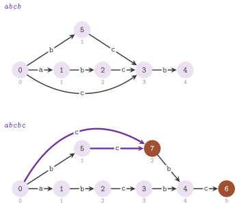
Building the automaton takes \(O( n )\) amortized time on a constant alphabet
(Blumer et al. 1985). In the library
the transitions of a state are a short vector of pairs (byte, state),
searched linearly, and the time is thus \(O( n \sigma )\) for \(\sigma\)
distinct bytes. contains() follows \(P\) from the start in
\(O( m \sigma )\). occurrences() gives the size of the end set of the
state of \(P\), counted once for all by adding the count of each state (1 if
it ends a prefix of \(S\), 0 for a clone) to its link, in decreasing order of
the lengths. distinctSubstrings() sums
\(\mathit{len}( v ) - \mathit{len}( \mathit{link}( v ) )\) over the states
but the start, by Lemma 15.28; and
longestCommonSubstring() scans a second string keeping the longest
suffix of its prefix that is a substring of \(S\), following the links on a
mismatch, in \(O( | T | \sigma )\).
The class is
// declarations of <ADS/string/SuffixAutomaton.h>
class SuffixAutomaton
{
 public:
 SuffixAutomaton( void );
 explicit SuffixAutomaton( std::string_view S );
 void extend( unsigned char c );
 [[nodiscard]] bool contains( std::string_view P ) const;
 [[nodiscard]] std::size_t occurrences( std::string_view P ) const;
 [[nodiscard]] std::size_t distinctSubstrings( void ) const;
 [[nodiscard]] std::pair< std::size_t , std::size_t >
 longestCommonSubstring( std::string_view T ) const;
 [[nodiscard]] std::size_t states( void ) const;
 [[nodiscard]] std::size_t size( void ) const;
 };
and, e.g., with the header ADS/string/SuffixAutomaton.h,
ADS::SuffixAutomaton A( "abcb" );
A.extend( 'c' );                         // the step of Figure 15.5
std::size_t s = A.states();              // s is 8, the start included
std::size_t k = A.occurrences( "bc" );   // k is 2
std::size_t t = A.distinctSubstrings();  // t is 12
15.5.5 Applications of the suffix arrays and trees¶
The functions of SuffixApplications.h solve on a suffix array or a
suffix tree the problems of Ferragina 2023, chapter
10 and their classical companions
(Gusfield 1997, §7.4 to §7.12;
Abouelhoda, Kurtz and Ohlebusch 2004).
They rest on one remark: a substring that occurs twice is a common prefix
of two suffixes, and the suffixes that share a prefix of length \(L\) are a
range of \(\mathit{SA}\) whose entries of \(\mathit{LCP}\) are all at least
\(L\). Hence a scan of \(\mathit{LCP}\), or a visit of the internal nodes of
the suffix tree, answers the questions on the repeats in \(O( n )\) time.
Lemma 15.29. The number of distinct nonempty substrings of \(T\) is
Proof. By definition, the substrings are the prefixes of the suffixes. The suffix \(\mathit{SA}[ r ]\) has \(n - \mathit{SA}[ r ]\) prefixes, of which the \(\mathit{LCP}[ r - 1 ]\) shortest are prefixes of the suffix before it, and all the others are prefixes of no smaller suffix (by Lemma 15.19). Summing over \(r\) gives (15.20). \(\square\)
longestRepeatedSubstring() is the largest entry of \(\mathit{LCP}\).
repeatedSubstring(), a query of text mining, finds a substring of length
\(L\) that occurs at least \(C\) times as a run of at least \(C - 1\) entries of
\(\mathit{LCP}\) that are at least \(L\), in one scan. longestCommonSubstring()
finds the longest substring common to at least \(k\) of \(m\) strings on the
suffix array of their join with \(m\) distinct separators (an integer
alphabet): a window of ranks that covers suffixes of \(k\) distinct strings,
slid by two pointers, has as common prefix the lce() of its two ends,
which gives \(O( N )\) time for \(N\) symbols in all (the generalized suffix
tree with the colors of Hui 1992 solves
it for all the values of \(k\) at once). maximalRepeats() gives the substrings that
occur twice and can be extended neither to the right (an internal node)
nor to the left (the symbols before their occurrences are not all equal,
or one occurrence starts the text), by one visit of the tree from the
leaves up. proximity() decides whether an occurrence of \(P\) and one of
\(Q\) lie within \(k\) places, which happens exactly when two adjacent ones of
different patterns do in their merged sorted list, in
\(O( | P | + | Q | + \mathit{occ} \log \mathit{occ} )\).
Lemma 15.30. Some occurrence of \(P\)
and some of \(Q\) lie within \(k\) places if and only if two consecutive items
of the merged sorted list of their places, one of each pattern, do; and
kMismatches() reports exactly the places with at most \(k\) mismatches.
Proof. If \(p\) and \(q\), of the two patterns, have \(| p - q | \le k\), the items of the list from \(p\) to \(q\) lie between them, and some two consecutive ones among them belong to different patterns, at distance at most \(| p - q |\); the converse is immediate. At a place \(s\), each longest common extension jumps over a maximal run of equal symbols of \(T[ s .. ]\) and \(P\), and the symbol after it, if any, is a mismatch; hence the \(j\)-th jump ends at the \(j\)-th mismatch, and the place has at most \(k\) mismatches if and only if at most \(k + 1\) jumps reach the end of \(P\). \(\square\)
kMismatches() finds the places where \(P\) occurs with at most \(k\)
substitutions (Landau and Vishkin 1986):
at each place, at most \(k + 1\) longest common extensions of a suffix of \(T\)
and a suffix of \(P\), both suffixes of \(T \# P\), jump over the matches,
each in \(O( 1 )\) by the range minima of its \(\mathit{LCP}\); hence
\(O( n k )\) time after \(O( n + m )\) preprocessing, against the \(O( n m )\)
of trying each place. lz77ByTree() computes the parsing of Ziv and
Lempel 1977: the phrase at \(i\) copies the
longest prefix of the suffix \(i\) that starts earlier, found by walking down
along the suffix \(i\) while the least leaf below the next node is smaller
than \(i\) (the least leaves are computed by one visit). Indeed, a suffix
that starts earlier and shares more than the depth of the node reached
would be a leaf below the next node. In the code the copy is taken from the least
leaf, the farthest occurrence, in \(O( n \log \sigma )\) time in all; the
phrase is the triple (distance, length, next symbol), a CopyPhrase
whose next symbol is empty at the end of the text, and
decodeCopyPhrases() inverts it.
The declarations of SuffixApplications.h are
// declarations of <ADS/string/SuffixApplications.h>
struct CopyPhrase
{
 std::size_t distance = 0;
 std::size_t length = 0;
 std::optional< char > next;
 friend bool operator==( const CopyPhrase & , const CopyPhrase & ) = default;
 };

[[nodiscard]] inline std::pair< std::size_t , std::size_t >
longestRepeatedSubstring( const SuffixArray & SA );
[[nodiscard]] inline std::optional< std::size_t >
repeatedSubstring( const SuffixArray & SA , std::size_t L , std::size_t C );
[[nodiscard]] inline std::uint64_t
distinctSubstrings( const SuffixArray & SA );
[[nodiscard]] inline std::string
longestCommonSubstring( const std::vector< std::string > & S , std::size_t k );
[[nodiscard]] inline std::vector< std::pair< std::size_t , std::size_t > >
maximalRepeats( const SuffixTree & ST );
[[nodiscard]] inline bool proximity( const SuffixArray & SA ,
                                     std::string_view P , std::string_view Q ,
                                     std::size_t k );
[[nodiscard]] inline std::vector< std::size_t >
kMismatches( std::string_view T , std::string_view P , std::size_t k );
[[nodiscard]] inline std::vector< CopyPhrase >
lz77ByTree( std::string_view T );
[[nodiscard]] inline std::string
decodeCopyPhrases( const std::vector< CopyPhrase > & Z );
where longestRepeatedSubstring() gives the place and the length of the
substring, distinctSubstrings() the count (15.20), and
maximalRepeats() the pairs (place, length). For instance, with the header
ADS/string/SuffixApplications.h,
ADS::SuffixArray S( "banana" );
auto [ p , l ] = ADS::longestRepeatedSubstring( S );  // "ana": l is 3
std::uint64_t d = ADS::distinctSubstrings( S );      // d is 15
std::string c = ADS::longestCommonSubstring( { "xabcy" , "zabcw" , "abq" } ,
                                             3 );  // c is "ab"
15.5.6 The engineered longest common extension¶
LceIndex of LongestCommonExtension.h answers
\(\mathrm{lce}( i , j )\), which SuffixArray::lce() computes as the range
minimum
in two stages; it builds \(\mathit{SA}\) by suffixArray() and
\(\mathit{LCP}\) by lcpArrayPhi(). First, the first 64 symbols of the two
suffixes are compared directly, 32 at a time by the vectors of Highway (8
without it):
on most texts most extensions are short. We prefer the direct comparison, which
reads two lines of the text, and may then be faster than any query that reads the
inverse and the LCP array at random (Ilie, Navarro and Tinta
2010 found it the fastest on the texts
with few long repeats). Second, the longer extensions go to a range
minimum on \(\mathit{LCP}\), cut into blocks of 16 entries, each one line of
the cache.
Lemma 15.31. For the entry \(r\) of a block that starts at \(s\), let the word \(M_r\) of 16 bits have the bit \(k\) set if \(\mathit{LCP}[ s + k ] < \mathit{LCP}[ s + k' ]\) for every \(k < k' \le r - s\). Then the minimum of \(\mathit{LCP}[ s + a .. r ]\) is \(\mathit{LCP}[ s + a + \mathrm{ctz}( M_r \gg a ) ]\).
Proof. The bits of \(M_r\) mark the entries that are smaller than all the entries after them up to \(r\), i.e., the stack of the suffix minima of the block up to \(r\). We see that the first marked place at or after \(s + a\) is smaller than everything after it up to \(r\), and not larger than anything between \(s + a\) and itself (an unmarked entry there has a smaller or equal entry after it, and so on up to a marked one); hence it is the minimum. \(\square\)
These are the words of Alstrup et al. 2002: one shift and one count of trailing zeros per block. In turn, the blocks form groups of 64, each with the sparse table of the minima of its blocks, and the minima of the groups are in a sparse table of their own. The blocks strictly between those of \(a\) and \(b - 1\) are covered by two overlapping ranges of one group, or by those of two partial groups and of the groups between them.
Every place that a query reads is known once the two ranks are, and the lines of the two blocks are requested with their words, and a query thus waits for two reads of the memory in a row: the ranks, then all the rest. Building the index costs \(O( n )\), but for the table of the groups, \(O( ( n / 1024 ) \log ( n / 1024 ) )\); a query costs \(O( 1 )\). In all, we use \(4 n\) bytes for each of \(\mathit{SA}^{-1}\) and \(\mathit{LCP}\) (on 32 bits), \(2 n\) for the words and \(1.75 n\) for the tables inside the groups, against the \(2 n + o( n )\) bits of the succinct range minima of Fischer and Heun 2011, whose practical form (Baumstark et al. 2017) pays for its space with a select on a sequence of balanced parentheses at each query.
The class is
// declarations of <ADS/string/LongestCommonExtension.h>
template< class I = std::uint32_t >
 requires( std::same_as< I , std::uint32_t > ||
           std::same_as< I , std::uint64_t > )
class LceIndex
{
 public:
 explicit LceIndex( std::string_view T );
 [[nodiscard]] std::size_t lce( std::size_t i , std::size_t j ) const;
 [[nodiscard]] std::size_t size( void ) const;
 };
and ADS::LceIndex<>( "banana" ).lce( 1 , 3 ) is 3.
15.6 Dictionaries searched by prefix¶
We now turn to a sorted array of \(n\) strings, the dictionary, in which one searches the strings prefixed by a pattern \(P\) of \(p\) symbols, as in the autocompletion of a query (Ferragina 2023, chapter 9). By Lemma 15.19, applied to the dictionary instead of the suffixes, those strings are consecutive, between the lexicographic position of \(P\) (the number of strings smaller than \(P\)) and that of \(P \#\).
15.6.1 The search by prefix¶
lexicographicPosition(), prefixEnd() and prefixRange() of
PrefixSearch.h search the array by two binary searches, \(O( p \log n )\)
time, each step a comparison of strings. This search is simple, but each
step reads a string far from the others, i.e., \(O( ( p / B ) \log n )\)
transfers of blocks of \(B\) symbols; the two-level dictionaries of
§15.6.2 reduce it to a search on a sample of
the strings and the scan of one bucket.
BinnedSearch is the search by interpolation of Demaine, Jones and
Pătrașcu 2004 in a sorted array \(X\) of
\(m\) integers. We cut the range \([ x_1 , x_m ]\) into bins of width
\(b = \lceil ( x_m - x_1 + 1 ) / m \rceil\), an array gives where each bin
starts in \(X\), and \(y\) is searched by a binary search in its bin
\(\lfloor ( y - x_1 ) / b \rfloor\).
Lemma 15.32. Let \(\Delta\) be the ratio of the largest to the smallest gap between consecutive items of \(X\). Then a bin holds \(O( \Delta )\) items, and a search takes \(O( \log \min( \Delta , m ) )\) time.
Proof. With \(g_{\min}\) and \(g_{\max}\) the smallest and the largest gap, \(x_m - x_1 \le ( m - 1 ) g_{\max}\), and so \(b \le ( x_m - x_1 ) / m + 1 \le g_{\max} + 1\). The items of a bin lie in an interval of \(b\) integers, at least \(g_{\min}\) apart, and they are thus at most \(( b - 1 ) / g_{\min} + 1 \le \Delta + 1\). The bin of \(y\) costs one division, and a binary search in at most \(\min( \Delta + 1 , m )\) items gives the bound. \(\square\)
Such a search is never worse than the binary search (up to a constant), and
it takes \(O( \log \log m )\) time with high probability on uniform keys, as
the search by interpolation of Perl, Itai and Avni
1978 (chapter 6), whose worst case is
\(O( m )\), at the price of the array of the bins. BinnedStringSearch
does the same on strings, read as the integers of their first 8 symbols
(padded with the symbol 0), which keep their order; the binary search in
a bin compares the strings in full. One can inspect the bins of BinnedSearch
by bins(), width() (the width \(b\)), bin() (the places of a
bin in \(X\)), binOf() (the bin of \(y\), none outside \([ x_1 , x_m ]\)),
largestBin(), size() and items(), and contains() decides whether
\(y\) is an item; keys() gives the BinnedSearch of the integers of the
strings of a BinnedStringSearch. Finally, commonPrefixLength() of
PrefixSearch.h is the length of the longest common prefix of two
strings, compared from their start, which the codings below use.
15.6.2 The front coding¶
Adjacent strings of a sorted dictionary share a prefix, and the front
coding of FrontCoding.h (Witten, Moffat and Bell
1999) writes the string \(s_i\) as the
pair \(( \ell_i , \hat s_i )\) (a FrontPair), where \(\ell_i\) is the length of the longest
common prefix of \(s_i\) and \(s_{i-1}\) (0 for the first one) and
\(\hat s_i\) the rest of \(s_i\) (Figure 15.6).
frontDecode() copies \(\ell_i\) symbols of the string before and appends
\(\hat s_i\):
We write the length in the byte-aligned code of Ferragina 2023, chapter
9 (encodeLength()): the binary of
\(\ell\) padded to a whole number \(k\) of bytes, with the first two bits of
the padding giving \(k - 1\), so that \(\ell < 2^{30}\) takes 1 to 4 bytes,
the most significant first:
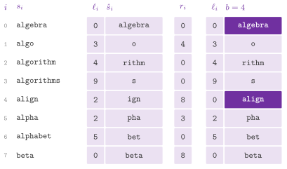
A string is decoded from the last string stored whole before it, and with
no other such string the decoding of \(s_i\) may scan all the dictionary
before it. FrontCodedDictionary therefore stores some strings whole (the
anchors) and decodes a string from the anchor before it, copying only
the \(\ell\) symbols that each pair takes from the previous string. Two
policies choose the anchors. bucketed() is the front coding with buckets
\(\mathit{FC}_B\) of Ferragina 2023:
an anchor every \(b\) strings, i.e., buckets of \(b\) strings coded on their
own. A larger \(b\) compresses better and scans more, up to \(\Theta( b^2 )\)
symbols for a bucket like \(a , aa , aaa , \ldots\).
localityPreserving() is the locality-preserving front coding of Bender,
Farach-Colton and Kuszmaul 2006, which
bounds the scan of each string by the length of that string: \(s_i\) is an anchor if it
is the first string, if \(\ell_i = 0\) (it then costs nothing more as an
anchor), or if more than \(c \, | s_i |\) symbols of the coding lie between
the previous anchor and \(s_i\). Our dictionary gives access() (a string,
decoded from the anchor before it), decodeCost() (the symbols of the
coding that access() reads), size(), anchors(), anchor() (the
place of an anchor), anchorString(), characters() (those of the rests
and of the anchors), bytes() (with the codes of the lengths), and a
forward iterator that decodes the strings one after the other, each from
the one before.
Theorem 15.4. With the policy of
localityPreserving() and \(c > 2\), a string \(s_i\) is decoded by reading
at most \(( c + 1 ) | s_i |\) symbols of the coding, and the coding takes at
most \(( 1 + 2 / ( c - 2 ) ) \, \mathit{FC}( D )\) symbols, where
\(\mathit{FC}( D ) = \sum_i | \hat s_i |\) is the size of the front coding
without anchors.
Proof. The decoding of \(s_i\) reads the coding from the anchor before it, which begins at most \(c | s_i |\) symbols back (otherwise \(s_i\) would be an anchor), plus at most \(| s_i |\) symbols of \(s_i\) itself. For the space, let \(C\) be the size of the coding and \(E = C - \mathit{FC}( D )\) its excess. An anchor \(s_i\) with \(\ell_i > 0\) costs \(\ell_i \le | s_i |\) symbols more than its front-coded pair, and it is chosen only when the coding from the previous anchor up to \(s_i\) holds more than \(c | s_i |\) symbols; the other anchors cost nothing more. These stretches of the coding are disjoint, and hence \(E \le \sum | s_i | < C / c = ( \mathit{FC}( D ) + E ) / c\), i.e., \(E < \mathit{FC}( D ) / ( c - 1 )\), which is at most \(2 \, \mathit{FC}( D ) / ( c - 2 )\) for \(c > 2\). \(\square\)
We remark that the proof gives the tighter factor \(c / ( c - 1 )\) for any \(c > 1\); the contracts check the bound of the statement, that of Bender, Farach-Colton and Kuszmaul 2006.
Thus the time of a decoding controls the space, and reading
\(( c + 1 ) | s_i |\) consecutive symbols costs the optimal
\(O( | s_i | / B )\) transfers of blocks. Both policies search by prefix as
the two-level scheme of Ferragina 2023, chapter
9: a binary search on the anchors,
which are stored in full, and the scan of the one bucket where the pattern falls,
decoded on the fly (the first level may be replaced by a Patricia trie on
the anchors, TwoLevelDictionary.h of chapter 7). The string B-tree of
Ferragina and Grossi 1999 and its
cache-oblivious version by Bender, Farach-Colton and Kuszmaul
2006, which also works on the
locality-preserving coding, bring the search in external memory to
\(O( ( p + \mathit{occ} ) / B + \log_B n )\) transfers.
15.6.3 The rear coding¶
In the rear coding of RearCoding.h we write, in place of \(\ell_i\),
\(r_i = | s_{i-1} | - \ell_i\), the symbols to take off the end of \(s_{i-1}\)
before appending \(\hat s_i\) (rearCode(), rearDecode(), the pairs
being of type RearPair). Both codings
decode a string from the one before and carry the same information; but
\(r_i\) is the smaller number where the strings share long prefixes (URLs,
paths, the words of a language), and a code of variable length takes fewer
bytes for it. Also, the rear coding is the variant of the front coding on which
Ferragina et al. 2008 build their
compressed dictionaries of strings for the external memory.
RearCodedDictionary is the front coding with buckets of the compressed
string dictionaries of Martínez-Prieto et al.
2016, in the rear coding and
with its symbols entropy-coded as in their HTFC, by a code of Huffman
instead of their code of Hu and Tucker (whose order the search does not
need, since it decodes the strings that it compares). It is one string of
bits in which each bucket of \(b\) strings begins with its first string and
goes on with a triple \(( r_i , | \hat s_i | , \hat s_i )\) per string. The
symbols, the rears and the lengths are each in a canonical code of Huffman
of their own frequencies (chapter 21). Their codewords have at most 11 bits,
whence a table of \(2^{11}\) entries decodes a symbol by one read of 11 bits
(and one of \(2^{12}\) entries up to 3 symbols by one read of 12); the places
of the buckets are kept by Elias-Fano (chapter 22). Moreover, the 16 bytes of each
first string that follow the prefix common to all the strings are kept
apart in two words, so that the binary search on the buckets decodes a
first string only when those bytes do not decide. With
\(\mathit{RC}_H( D )\) the bits of the coding, the dictionary takes
besides the directory of Elias-Fano and the three tables of decoding, the
128 bits being those of the two words of each bucket. Our constructor
takes \(b\), 16 by default (bucketSize()); codeBytes() gives the bytes
of \(\mathit{RC}_H( D )\) and bytes() all of them, and besides
access(), lexicographicPosition(), prefixEnd() and prefixRange()
the dictionary answers lookup() (the place of a string, size() if it
is absent) and empty(); the private constants kMax \(= 11\), kWide
\(= 12\) and kHead \(= 16\) are the bounds above.
In the scan of a bucket we compare a string with the pattern \(Q\) only when it must, and rebuild no string (Algorithm 15.12).
Lemma 15.33. Let the current string \(s\) be smaller than \(Q\) and share with it a prefix of \(\lambda\) symbols, and let the next string keep \(\kappa = | s | - r\) symbols of \(s\). If \(\kappa > \lambda\), the next string is smaller than \(Q\) too, and it shares with \(Q\) the same \(\lambda\) symbols.
Proof. The next string has the symbol \(s[ \lambda ]\) at the place \(\lambda\), which is below \(Q[ \lambda ]\) since \(s < Q\) and \(s\) is not a prefix of \(Q\) (it has more than \(\lambda\) symbols); hence the next string is smaller than \(Q\) and agrees with it exactly on the first \(\lambda\) symbols. \(\square\)
Only a string that keeps at most \(\lambda\) symbols is compared, from the place where its rest begins and while that rest is decoded. A search thus costs \(O( | Q | \log ( n / b ) )\) for the binary search and \(O( | Q | + \sum_i | \hat s_i | )\) for the bucket. We declare the three headers of the section as
// declarations of <ADS/string/PrefixSearch.h> <ADS/string/FrontCoding.h>
//                  <ADS/string/RearCoding.h>
[[nodiscard]] inline std::size_t
lexicographicPosition( const std::vector< std::string > & A ,
                       std::string_view Q );
[[nodiscard]] inline std::size_t
prefixEnd( const std::vector< std::string > & A , std::string_view P );
[[nodiscard]] inline std::pair< std::size_t , std::size_t >
prefixRange( const std::vector< std::string > & A , std::string_view P );
[[nodiscard]] inline std::size_t commonPrefixLength( std::string_view a ,
                                                     std::string_view b );

class BinnedSearch
{
 public:
 explicit BinnedSearch( std::vector< std::uint64_t > X );
 [[nodiscard]] std::size_t position( std::uint64_t y ) const;
 [[nodiscard]] bool contains( std::uint64_t y ) const;
 [[nodiscard]] std::size_t bins( void ) const;
 [[nodiscard]] std::uint64_t width( void ) const;
 [[nodiscard]] std::pair< std::size_t , std::size_t >
 bin( std::size_t j ) const;
 [[nodiscard]] std::optional< std::size_t > binOf( std::uint64_t y ) const;
 [[nodiscard]] std::size_t largestBin( void ) const;
 [[nodiscard]] std::size_t size( void ) const;
 [[nodiscard]] const std::vector< std::uint64_t > & items( void ) const;
 };

class BinnedStringSearch
{
 public:
 explicit BinnedStringSearch( std::vector< std::string > A );
 [[nodiscard]] std::size_t lexicographicPosition( std::string_view Q ) const;
 [[nodiscard]] std::size_t prefixEnd( std::string_view P ) const;
 [[nodiscard]] std::pair< std::size_t , std::size_t >
 prefixRange( std::string_view P ) const;
 [[nodiscard]] const BinnedSearch & keys( void ) const;
 };

using FrontPair = std::pair< std::size_t , std::string >;
[[nodiscard]] inline std::vector< FrontPair >
frontCode( const std::vector< std::string > & D );
[[nodiscard]] inline std::vector< std::string >
frontDecode( const std::vector< FrontPair > & F );
inline void encodeLength( std::uint32_t l , std::string & out );
[[nodiscard]] inline std::uint32_t decodeLength( std::string_view in ,
                                                 std::size_t & pos );

class FrontCodedDictionary
{
 public:
 [[nodiscard]] static FrontCodedDictionary
 bucketed( const std::vector< std::string > & D , std::size_t b );
 [[nodiscard]] static FrontCodedDictionary
 localityPreserving( const std::vector< std::string > & D , double c );
 [[nodiscard]] std::string access( std::size_t i ) const;
 [[nodiscard]] std::size_t decodeCost( std::size_t i ) const;
 [[nodiscard]] std::size_t lexicographicPosition( std::string_view Q ) const;
 [[nodiscard]] std::size_t prefixEnd( std::string_view P ) const;
 [[nodiscard]] std::pair< std::size_t , std::size_t >
 prefixRange( std::string_view P ) const;
 [[nodiscard]] std::size_t rankInBucket( std::size_t k , std::string_view P ,
                                         bool upper ) const;
 [[nodiscard]] std::size_t size( void ) const;
 [[nodiscard]] std::size_t anchors( void ) const;
 [[nodiscard]] std::size_t anchor( std::size_t k ) const;
 [[nodiscard]] std::string_view anchorString( std::size_t k ) const;
 [[nodiscard]] std::size_t characters( void ) const;
 [[nodiscard]] std::size_t bytes( void ) const;
 };

using RearPair = std::pair< std::size_t , std::string >;
[[nodiscard]] inline std::vector< RearPair >
rearCode( const std::vector< std::string > & D );
[[nodiscard]] inline std::vector< std::string >
rearDecode( const std::vector< RearPair > & R );

class RearCodedDictionary
{
 public:
 RearCodedDictionary( void ) = default;
 explicit RearCodedDictionary( const std::vector< std::string > & D ,
                               std::size_t b = 16 );
 [[nodiscard]] std::size_t size( void ) const;
 [[nodiscard]] bool empty( void ) const;
 [[nodiscard]] std::size_t bucketSize( void ) const;
 [[nodiscard]] std::string access( std::size_t i ) const;
 [[nodiscard]] std::size_t lookup( std::string_view Q ) const;
 [[nodiscard]] std::size_t lexicographicPosition( std::string_view Q ) const;
 [[nodiscard]] std::size_t prefixEnd( std::string_view P ) const;
 [[nodiscard]] std::pair< std::size_t , std::size_t >
 prefixRange( std::string_view P ) const;
 [[nodiscard]] std::size_t codeBytes( void ) const;
 [[nodiscard]] std::size_t bytes( void ) const;
 };
where rankInBucket( k , P , upper ) places \(P\) (or \(P \#\), if upper) in
the bucket \(k\), and FrontCodedDictionary has the forward iterators begin()
and end(). For instance, with the headers ADS/string/FrontCoding.h and
ADS/string/RearCoding.h, the dictionary of Figure
15.6 gives
std::vector< std::string > D = { "algebra" ,    "algo" ,  "algorithm" ,
                                 "algorithms" , "align" , "alpha" ,
                                 "alphabet" ,   "beta" };
auto F = ADS::FrontCodedDictionary::bucketed( D , 4 );  // anchors 0 and 4
auto [ lo , hi ] = F.prefixRange( "algo" );             // lo is 1, hi is 4
std::string s = F.access( 3 );                         // s is "algorithms"
ADS::RearCodedDictionary R( D );
std::size_t k = R.lookup( "alpha" );  // k is 5
Algorithm 15.12. The lexicographic
position in RearCodedDictionary.
15.7 Palindromes, Lyndon words, parentheses and anagrams¶
15.7.1 Palindromes¶
A palindrome reads the same in both directions. Palindromes.h has the
algorithms of the textbooks for three problems on a sequence \(s\) of \(n\)
items, and the eertree. The longest palindromic substring
(longestPalindromicSubstring()) is found by the algorithm of Manacher
1975, which computes the radius of the
longest palindrome about each of the \(2 n - 1\) centres. It keeps the
palindrome \([ l , r )\) found so far whose right end is the largest: a
centre \(i < r\) starts from the radius of its mirror \(l + r - 1 - i\),
capped at \(r - i\), since the palindrome is symmetric, and compares only the
items past \(r\).
Lemma 15.34. The algorithm of Manacher takes \(\Theta( n )\) time and space.
Proof. As in Lemma 15.5: inside \([ l , r )\) the palindrome about \(i\) is the mirror of the one about \(l + r - 1 - i\), as far as \(r\); each successful comparison past \(r\) moves \(r\) forward, at most \(n\) times for each of the two loops (the odd and the even centres), and each centre has at most one failed comparison. \(\square\)
By contrast, the dynamic programming of the textbook fills the table of the palindromes \(s[ i .. j ]\) by increasing length in \(\Theta( n^2 )\) time and space, and the expansion about each centre takes \(O( n^2 )\) time and \(O( 1 )\) space; the suffix tree of \(s\) and of its reverse gives the same answer in linear time with a much larger constant.
For the longest palindromic subsequence (longestPalindromicSubsequence()) we
have \(\mathit{DP}[ i ][ j ]\), its length for \(s[ i .. j ]\), equal to 1 if
\(i = j\), to \(\mathit{DP}[ i + 1 ][ j - 1 ] + 2\) if \(s_i = s_j\), and to the
larger of \(\mathit{DP}[ i + 1 ][ j ]\) and \(\mathit{DP}[ i ][ j - 1 ]\)
otherwise, \(\Theta( n^2 )\) time and space; it is the longest common
subsequence of \(s\) and of its reverse; the algorithms of
§15.4.5 apply to it too. The fewest
palindromes into which \(s\) can be cut (palindromicPartition()) satisfy
\(D[ j ] = \min \{ D[ i ] + 1 : s[ i .. j ) \text{ a palindrome} \}\),
\(D[ 0 ] = 0\). While the textbook builds the table of the palindromes first, here
each palindrome relaxes \(D[ j ]\) while the expansion about its centre finds
it, the centres taken from left to right, so that \(D[ i ]\) is final when it
is used: \(O( n^2 )\) time and \(O( n )\) space.
We also give the eertree (palindromic tree) of Rubinchik and Shur
2018 (Eertree), which has a node for each
distinct nonempty palindrome of the string, two roots of lengths \(-1\) and
0, the edge \(c\) from \(v\) to \(c v c\), and the suffix link of \(v\) to its
longest proper palindromic suffix.
Lemma 15.35. A symbol appended to a string creates at most one new palindrome, its longest palindromic suffix; hence a string of \(n\) symbols has at most \(n\) distinct nonempty palindromes.
Proof. A shorter palindromic suffix \(x\) of the new string \(s c\) is a suffix of its longest one \(y\), and hence (by the symmetry of \(y\)) also a prefix of \(y\), which occurred before \(c\) was appended. \(\square\)
add() finds the longest palindromic suffix of the new string on the
suffix links of the previous one (and returns whether it is a new
palindrome), distinct() gives the number of distinct nonempty
palindromes, suffixLength() the length of the longest palindromic
suffix and size() that of the string; add() takes \(O( 1 )\) amortized steps on a constant
alphabet (the edges of a node are a short vector, \(O( \sigma )\) each).
palindromicFactorization() gives the fewest palindromes of a partition
in \(O( n \log n )\) time (Fici et al. 2014;
Rubinchik and Shur 2018). The
lengths of the palindromic suffixes of a prefix form \(O( \log n )\)
arithmetic series, along which the difference
\(\mathit{diff}( v ) = \mathit{len}( v ) - \mathit{len}( \mathit{link}( v ) )\)
is constant; the series link of \(v\) leads to the first node past its
series. At the place \(i\), the best value of a series is the best of the
same series at \(i - \mathit{diff}( v )\) together with its shortest
palindrome,
the second term only when \(\mathit{diff}( v ) = \mathit{diff}( \mathit{link}( v ) )\), which costs \(O( 1 )\) per series.
We declare the functions of Palindromes.h on any sequence S, with an
overload on std::string for each but the first, as
// declarations of <ADS/string/Palindromes.h>
template< class S >
 requires std::is_class_v< S >
[[nodiscard]] std::pair< std::size_t , std::size_t >
longestPalindrome( const S & s );
template< class S >
 requires std::is_class_v< S >
[[nodiscard]] S longestPalindromicSubstring( const S & s );
template< class S >
 requires std::is_class_v< S >
[[nodiscard]] S longestPalindromicSubsequence( const S & s );
template< class S >
 requires std::is_class_v< S >
[[nodiscard]] std::vector< S > palindromicPartition( const S & s );

class Eertree
{
 public:
 Eertree( void );
 explicit Eertree( std::string_view s );
 bool add( unsigned char c );
 [[nodiscard]] std::size_t distinct( void ) const;
 [[nodiscard]] std::size_t suffixLength( void ) const;
 [[nodiscard]] std::size_t size( void ) const;
 };

[[nodiscard]] inline std::vector< std::string >
palindromicFactorization( std::string_view s );
where longestPalindrome() gives the start and the length. For instance,
with the header ADS/string/Palindromes.h,
std::string p = ADS::longestPalindromicSubstring( std::string( "abacabad" ) );
// p is "abacaba"
ADS::Eertree E( "abacabad" );
std::size_t k = E.distinct();  // k is 8: a, b, c, d, aba, aca,
                               // bacab, abacaba
15.7.2 Lyndon words¶
A Lyndon word is a nonempty string strictly smaller than all its proper rotations (equivalently, than all its proper suffixes). By the theorem of Chen, Fox and Lyndon 1958, every string \(S\) has exactly one factorization
into Lyndon words; e.g., \(\texttt{banana} = \texttt{b} \cdot \texttt{an}
\cdot \texttt{an} \cdot \texttt{a}\). The algorithm of Duval
1983 (lyndonFactorization() of
Lyndon.h) keeps \(S = s_1 s_2 s_3\), with \(s_1\) factored and
\(s_2 = w^h w'\) for a Lyndon word \(w\) and a proper prefix \(w'\) of \(w\). It
compares the next symbol \(c\) of \(s_3\) with the one \(| w |\) places before
it: if equal, \(w'\) grows; if larger, \(s_2 c\) is a Lyndon word and becomes
\(w\); if smaller, the \(h\) copies of \(w\) are factors of (15.24) and the scan
resumes after them (Algorithm 15.13).
Algorithm 15.13. The factorization of Duval 1983 and the least rotation.
Lemma 15.36. The factorization (15.24) is unique, and the algorithm of Duval returns it, in at most \(2 n\) comparisons and \(O( 1 )\) space besides the factors.
Proof. We use two facts on a Lyndon word \(w\). First, \(w\) has no border: a proper suffix \(x\) of \(w\) that were also a prefix would be smaller than \(w\), a longer word that it starts, against \(w < x\). Hence \(w\) and each proper suffix \(x\) of it differ at some place \(t < | x |\), with \(x[ t ] > w[ t ]\); in particular, no symbol of \(w\) is smaller than \(w[ 0 ]\).
Uniqueness. In a factorization (15.24), \(w_1\) is the longest prefix of \(S\) that is a Lyndon word. Otherwise, a longer Lyndon prefix would be \(y = w_1 \cdots w_i x\) with \(i \ge 1\) and \(x\) a nonempty prefix of \(w_{i+1}\); then \(x \le w_{i+1} \le w_1 \le y\), the first and the last since a prefix is not larger than the word, while \(y < x\) since \(x\) is a proper suffix of \(y\). Hence \(w_1\) is determined by \(S\), and by induction on the length so are the other factors.
Correctness. A run of lines 4 to 7 from the place \(i\) keeps the invariant that \(S[ i .. j - 1 ] = w^h w'\), with \(w = S[ i .. i + p - 1 ]\) a Lyndon word, \(p = j - k\), \(h \ge 1\) and \(w'\) a proper prefix of \(w\); it holds at the start, with \(w = S[ i ]\) and \(w'\) empty. Line 5 compares \(c = S[ j ]\) with \(S[ k ] = S[ j - p ] = w[ | w' | ]\). If they are equal, \(w' c\) is a prefix of \(w\), or \(w\) itself (and \(h\) grows by 1), and \(k\) and \(j\) advance together. If \(c > w[ | w' | ]\), we show that \(z = w^h w' c\) is a Lyndon word, which line 6 makes the new \(w\), with \(h = 1\) and \(p = j + 1 - i\). Let \(x\) be a proper suffix of \(z\). If \(x = w^g w' c\) with \(0 \le g \le h\), then \(z\) and \(x\) agree on \(w^g w'\) and differ next, where \(z\) has \(w[ | w' | ] < c\). Otherwise \(x\) starts at a place \(r \ge 1\) of a copy of \(w\), or at a place \(1 \le r \le | w' |\) of \(w'\) (the place \(| w' |\) being that of \(c\)), and \(y = w[ r .. p - 1 ]\), a proper suffix of \(w\), differs from \(w\) first at a place \(t < | y |\), with \(y[ t ] > w[ t ]\). If \(x\) starts in a copy of \(w\), it starts with \(y\), and \(x > z\) by the place \(t\). If it starts in \(w'\), then \(x = w[ r .. | w' | - 1 ] c\): when \(t < | w' | - r\), the place \(t\) decides as before; when \(t \ge | w' | - r\), the two agree on the first \(| w' | - r\) places and \(x\) has there \(c > w[ | w' | ] = y[ | w' | - r ] \ge w[ | w' | - r ] = z[ | w' | - r ]\). In all cases \(x > z\).
The run stops at \(j = n\) or at \(c < w[ | w' | ]\), and line 8 outputs \(h\) copies of \(w\), since \(i \le k\) holds exactly for \(i = i_0 , i_0 + p , \ldots , i_0 + ( h - 1 ) p\), \(i_0\) the start of the run, and the next run starts at the place of \(w'\). Each factor is thus a Lyndon word, the copies of a run are equal, and a factor \(x\) of the next run is not larger than \(w\): \(x\) is a prefix of the rest of the string from the place of \(w'\), and either it is a prefix of \(w'\), hence of \(w\), or it starts with \(w' c\), which is smaller than \(w\) at the place \(| w' |\). The factors cover \(S\), since each run outputs at least one; by the uniqueness, they are (15.24).
Cost. A run from \(i\) makes one comparison for each value of \(j\) from \(i + 1\) to the place \(j\) where it stops, i.e., at most \(j - i\) comparisons, and \(j - i < ( h + 1 ) | w | \le 2 h | w |\); the next run starts at \(i + h | w |\), so that the comparisons of a run are at most twice the symbols that it moves past, and at most \(2 n\) in all. The space is that of \(i\), \(j\) and \(k\). \(\square\)
leastRotation() gives the start of the lexicographically least rotation
of \(S\) (the first one, if several) by the same scan on \(S S\): the least
rotation starts at the start of the factor of \(S S\) that covers the place
\(n\), in \(O( n )\) time (Duval 1983). Finally, isLyndon() decides whether a string is a
Lyndon word by the definition, comparing it with each of its proper
suffixes in \(O( n^2 )\) time; the contracts check by it the factors of
lyndonFactorization(). We declare them as
// declarations of <ADS/string/Lyndon.h>
[[nodiscard]] inline bool isLyndon( std::string_view S );
[[nodiscard]] inline std::vector< std::size_t >
lyndonFactorization( std::string_view S );
[[nodiscard]] inline std::size_t leastRotation( std::string_view S );
where lyndonFactorization() gives the starts of the factors, e.g.,
\(( 0 , 1 , 3 , 5 )\) for \(\texttt{banana}\).
15.7.3 Parentheses and anagrams¶
Parentheses.h finds the longest balanced strings of parentheses in a
text of \(n\) symbols, where open and close are the two parentheses and
any other symbol is neither. For the longest balanced subsequence
(longestBalancedSubsequence()), a scan matches each close with the
nearest open still unmatched before it, and the length is twice the
number of pairs matched, in \(\Theta( n )\) time and \(O( 1 )\) space (the interval recursion of the
textbook, the pair of the two ends or the best split, takes
\(\Theta( n^3 )\)). For the longest balanced substring
(longestBalancedSubstring()), a stack keeps the places of the opens not
matched yet: when a close matches the top, the substring from just after
the open still unmatched below it (or from the last place where the
balance broke) to the close is balanced, and it is the longest one ending
there; \(\Theta( n )\) time and \(O( n )\) space, while two scans of the counts
of opens and closes, from left to right and from right to left, need only
\(O( 1 )\) space.
Lemma 15.37. The scan of
longestBalancedSubsequence() matches as many pairs as a balanced
subsequence can have.
Proof. The scan matches a pair at each close but the \(u\) closes that find no open pending. Let \(x\) be the last of these closes. When the scan meets \(x\), each open before it has been matched to a close before it, and so the prefix up to \(x\) holds at least \(u\) closes more than opens. In a balanced subsequence each close follows the open matched to it, and so at least \(u\) closes of that prefix are left out; hence it has at most as many pairs as the closes less \(u\), which is the number that the scan matches. \(\square\)
We declare the two functions as
// declarations of <ADS/string/Parentheses.h>
[[nodiscard]] inline std::size_t
longestBalancedSubsequence( std::string_view s , char open = '(' ,
                            char close = ')' );
[[nodiscard]] inline std::pair< std::size_t , std::size_t >
longestBalancedSubstring( std::string_view s , char open = '(' ,
                          char close = ')' );
the second returning the start and the length.
Two words are anagrams if one is a permutation of the other.
anagramGroups() of Anagrams.h gives each word its signature, i.e.,
its items sorted, and gathers the words of equal signature in a hash table
(Bentley 2000, column 2):
\(O( n k \log k )\) expected time and \(O( n k )\) space for \(n\) words of
length at most \(k\), the groups in the order of their first word. A
signature by counting sort over \(\sigma\) symbols (or the vector of the
counts) costs \(O( k + \sigma )\) per word instead, and sorting the pairs
(signature, word) in place of hashing them gives the classes in
\(O( n k \log n )\) worst-case time.
The function has an overload on the strings:
// declarations of <ADS/string/Anagrams.h>
template< class S , class Hash = std::hash< S > >
[[nodiscard]] std::vector< std::vector< S > >
anagramGroups( const std::vector< S > & words );
15.8 Segmentations, cuts and the code of Huffman¶
15.8.1 Segmentations¶
A string \(s\) with no spaces is a sequence of words of a dictionary if and
only if some prefix \(s[ 0 .. j )\) is and \(s[ j .. i )\) is a word for
\(i = n\) (Montresor 2025, exercise 13.13).
wordBreak() of WordBreak.h fills \(\mathit{DP}[ i ]\), true when
\(s[ 0 .. i )\) is a sequence of words, for each \(i\), with
\(\mathit{DP}[ 0 ]\) true: \(O( n^2 )\) lookups, or \(O( n w )\) if no word is
longer than \(w\), and the words are read back from the table.
The dictionary is a predicate, and the words are returned in order:
// declarations of <ADS/string/WordBreak.h>
template< class F >
std::optional< std::vector< std::string > >
wordBreak( const std::string & s , F && lookup ,
           std::size_t longest = std::string::npos ,
           long * lookups = nullptr );
We count the segmentations (countSegmentations() of
Segmentations.h) by adding, instead, the counts of the words that start at
each place: \(D[ i ]\), the number of segmentations of \(X[ i .. n )\), is the
sum of \(D[ i + | w | ]\) over the words \(w\) that occur at \(i\), with
\(D[ n ] = 1\), filled from the right in \(O( n \sum_w | w | )\) time. With
the automaton of §15.3 the occurrences come in
one scan, and the time drops to \(O( n + \sum_w | w | + \mathit{occ} )\).
The readings of a string of digits as letters, \(A = 1 , \ldots , Z = 26\)
(countDecodings()), are its segmentations into the words \(1 , \ldots ,
26\): \(D[ i ] = 0\) if \(d_i = 0\), and otherwise \(D[ i + 1 ]\) plus
\(D[ i + 2 ]\) if \(d_i d_{i+1}\) is in \(10 .. 26\), in \(\Theta( n )\) time and
\(O( 1 )\) space. On \(n\) digits 1 the count is the Fibonacci number
\(F_{n+1}\), since then \(D[ i ] = D[ i + 1 ] + D[ i + 2 ]\); the counts grow
exponentially, and they are given modulo \(2^{64}\).
We declare them as
// declarations of <ADS/string/Segmentations.h>
template< class S >
 requires std::is_class_v< S >
[[nodiscard]] std::uint64_t
countSegmentations( const S & X , const std::vector< S > & words );
[[nodiscard]] inline std::uint64_t
countDecodings( const std::vector< int > & digits );
with an overload of the first on std::string; e.g.,
ADS::countDecodings( { 2 , 2 , 6 } ) is 3 (BBF, BZ, VF).
15.8.2 The cuts of a string¶
A string of length \(L\) has to be cut at the places
\(0 < w_1 < \cdots < w_n < L\). Each cut costs the length of the piece
that it splits (StringBreaking.h, Cormen et al. 2009, problem
15-9). With \(w_0 = 0\) and
\(w_{n+1} = L\), the least cost \(D[ i ][ j ]\) of the cuts strictly between
\(w_i\) and \(w_j\) is 0 for \(j = i + 1\) and otherwise
the scheme of the chain of matrices and of the optimal search tree, in \(\Theta( n^3 )\) time.
Lemma 15.38. Let \(K[ i ][ j ]\) be the largest \(k\) that attains the minimum of (15.25). Then \(K[ i ][ j - 1 ] \le K[ i ][ j ] \le K[ i + 1 ][ j ]\), and (15.25) can be filled in \(\Theta( n^2 )\) time.
Proof. The cost \(c( i , j ) = w_j - w_i\) satisfies the quadrangle inequality \(c( i , j ) + c( i' , j' ) \le c( i' , j ) + c( i , j' )\) for \(i \le i' \le j \le j'\) (as an equality), and it is monotone on the inclusion of the intervals; by Yao 1980 (after Knuth 1971 for the search trees) the largest optimal split is then monotone as stated. Restricting the search of \(k\) to \([ K[ i ][ j - 1 ] , K[ i + 1 ][ j ] ]\), the candidates of all the intervals of one length \(d\) telescope to \(K[ n + 2 - d ][ n + 1 ] - K[ 0 ][ d - 1 ] + O( n ) = O( n )\), and there are \(O( n )\) lengths. \(\square\)
Line 7 takes the largest optimal split, as the code does by the test \(\le\):
stringBreakingOrder() reads an optimal order of the cuts back from the
splits, each cut before those of its two pieces.
The two functions, with an overload on std::int64_t, are
// declarations of <ADS/string/StringBreaking.h>
template< class I >
[[nodiscard]] I stringBreakingCost( const std::vector< I > & cuts ,
                                    std::type_identity_t< I > length );
template< class I >
[[nodiscard]] std::vector< I >
stringBreakingOrder( const std::vector< I > & cuts ,
                     std::type_identity_t< I > length );
and, e.g., the cuts at 2, 8 and 10 of a string of 20 cost
ADS::stringBreakingCost( std::vector< int >{ 2 , 8 , 10 } , 20 ) \(= 38\).
15.8.3 The code of Huffman¶
A prefix code assigns to each character a string of bits, no one being a
prefix of another, and a text coded by it can thus be decoded; the code of
Huffman 1952 (huffman() of
Huffman.h, Montresor 2025, §14.4)
has the least expected length for the frequencies of the characters. The
characters go into a min-heap by frequency; the two least frequent ones,
\(c_1\) and \(c_2\), are replaced by a new virtual character of frequency
\(f_1 + f_2\) whose children in a binary tree are \(c_1\) and \(c_2\), and after
\(n - 1\) steps the root is left (Figure 15.7). The
code of a character is the path from the root to its leaf, 0 to the left
and 1 to the right (a single character gets the code 0):
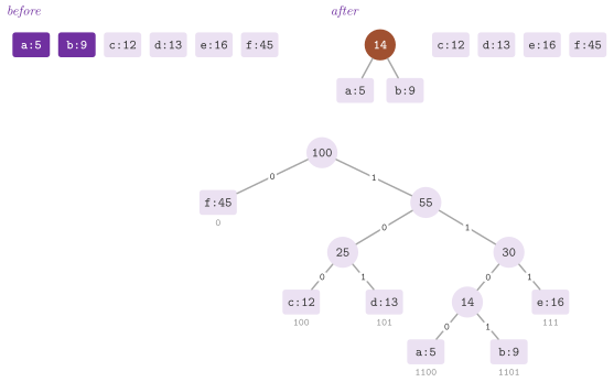
Theorem 15.5. The code of Huffman has the
least expected length among the prefix codes of the given frequencies, and
huffman() computes it in \(O( n \log n )\) time for \(n\) characters.
Proof. Some optimal tree has the two least frequent characters as sibling leaves at the largest depth, since exchanging them with the leaves there does not increase the cost. Moreover, the cost of a tree in which they are siblings differs from the cost of the tree with the two merged into one leaf of frequency \(f_1 + f_2\) by \(f_1 + f_2\), a constant; hence, by induction on the number of characters, the greedy choice is optimal. Each of the \(n - 1\) steps makes \(O( 1 )\) operations on a heap of \(O( n )\) items. \(\square\)
encode() concatenates the codes of the characters of a text, and
decode() follows the bits on the tree of the code, a character at each
leaf. Finally, the canonical codes and the codes of limited length that the
compressors of the library use are in chapter 21.
The three functions are
// declarations of <ADS/string/Huffman.h>
template< class C , class F >
std::map< C , std::string > huffman( const std::map< C , F > & freq );
template< class C >
std::string encode( const std::basic_string< C > & text ,
                    const std::map< C , std::string > & code );
template< class C >
std::basic_string< C > decode( const std::string & bits ,
                               const std::map< C , std::string > & code );
and the code of Figure 15.7 comes from, with the
header ADS/string/Huffman.h,
std::map< char , int > f = { { 'a' , 5 } ,  { 'b' , 9 } ,  { 'c' , 12 } ,
                            { 'd' , 13 } , { 'e' , 16 } , { 'f' , 45 } };
std::map< char , std::string > C = ADS::huffman( f );  // C[ 'a' ] is 1100
std::string b = ADS::encode( std::string( "face" ) , C );
std::string t = ADS::decode( b , C );  // t is "face"
15.9 Discussion and references¶
The exact search of one pattern is treated at length by Gusfield
1997 and by Charras and Lecroq
2004, and Faro and Lecroq
2013 survey the algorithms of the last
decades, among which the packed filters and the hashed q-grams that
StringSearcher combines; the fallback on the Two-Way algorithm, which
makes the worst case linear without the memory of the automata, is the
choice of several C libraries for memmem(). The automaton of Aho and
Corasick 1975 remains the reference for
many patterns, and the filters of MultiSearcher are those of the FDR
matcher of Hyperscan (Wang et al. 2019).
The dynamic programming of §15.4 follows chapter
13 of Montresor 2025; its
engineered form rests on Myers 1999,
Hyyrö 2003 and Ukkonen
1985a, as in edlib (Šošić and Šikić
2017), and on the diagonal transitions
of Landau and Vishkin 1989 and Myers
1986, as in the wavefront alignment
(Marco-Sola et al. 2021). In the
library there are no affine gap costs and no alignment of more than two strings.
The suffix array is from Manber and Myers 1993
and Gonnet, Baeza-Yates and Snider 1992;
Puglisi, Smyth and Turpin 2007
classify its constructions, of which SA-IS (Nong, Zhang and Chan
2011) and DivSufSort (Fischer and Kurpicz
2017) are the methods of the libraries
in use, the engineered suffixArray() combining the two. As for the indexes, the suffix tree
goes back to Weiner 1973 and
McCreight 1976, the suffix
automaton to Blumer et al. 1985 and
Crochemore 1986, and the
replacement of the suffix tree by a suffix array with its LCP array to
Abouelhoda, Kurtz and Ohlebusch 2004.
Instead, the compressed indexes (the FM-index and the Burrows-Wheeler transform) are
in chapter 21, and the succinct trees and the rank and select on which
they rest in chapter 22. The dictionaries of §15.6
follow chapter 9 of Ferragina 2023,
Bender, Farach-Colton and Kuszmaul 2006
and Martínez-Prieto et al. 2016;
the tries and the Patricia trie of a dictionary are in chapter 7. The
comparison of the engineered searches, distances, suffix arrays,
extensions and dictionaries with the libraries they are meant to compete
with (the C library and Boost.Algorithm, Vectorscan, edlib and
rapidfuzz-cpp, libsais and libdivsufsort, sdsl-lite) belongs to the
campaign of benchmarks of appendix B, and it is not reported here.
15.10 Exercises¶
Each exercise names the test of the library that solves it (run it with
ctest -R <name>).
- Find the occurrences of a pattern by trying each shift and by the
algorithm of Knuth, Morris and Pratt, and check that the second never
moves back in the text. Test:
beyond.string-matching. - Compute the strong failure function and check that
kmpStrong()never compares a symbol of the text twice with the same symbol of the pattern. Test:beyond.kmp-strong. - Implement the algorithms of Boyer and Moore, of Horspool, Shift-Or and
the Z-function, and check them against the naive search. Test:
engineered_strings.classic-matching. - Search a pattern by a filter of probes, by the shifts of its q-grams
and, when the filters let too much through, by the Two-Way algorithm,
in \(O( n + m )\) time on any text. Test:
engineered_strings.string-search. - Build the automaton of Aho and Corasick and report all the occurrences
of a set of patterns in one scan. Test:
engineered_strings.aho-corasick. - Put a filter of shuffles of bytes, or of shift-or on super characters,
in front of the automaton, so that no occurrence is missed. Test:
engineered_strings.multi-search. - Find the best approximate occurrence of a pattern by the table (15.10),
and walk back to where it starts (Montresor 2025, §13.1 and exercise
13.1). Tests:
ch13.sec13.1.matching,ch13.ex13.1. - Compute a longest common subsequence, the longest common substring and
the differences of two sequences (Montresor 2025, §13.7, exercises 13.2
and 13.10). Tests:
ch13.sec13.7.lcs,ch13.ex13.2,ch13.ex13.10. - Compute the global, semiglobal and local alignments of two strings
(Montresor 2025, exercises 13.7 to 13.9).
Tests:
ch13.ex13.7,ch13.ex13.8,ch13.ex13.9. - Decide whether a string is a shuffle of two others, and compute a
shortest common supersequence, the occurrences of a subsequence and the
LCS of three strings. Tests:
lib_strings.interleaving,lib_strings.supersequence,lib_strings.subsequence-occurrences,lib_strings.lcs3. - Compute the edit distance, the length of the LCS and the approximate
occurrences by the bit vectors of Myers and the diagonal transitions,
and check them against the tables. Test:
engineered_strings.edit-distance. - Build a suffix array by the six constructions, its LCP array by the
algorithm of Kasai et al., and search a pattern by the binary search
and by that of Manber and Myers. Tests:
pearls_suffix.sec10.2.3.constructions,pearls_suffix.sec10.2.2.kasai,pearls_suffix.sec10.2.1.search; the arrays of \(\texttt{mississippi}\) of the figures of Ferragina 2023, chapter 10 are checked bypearls_suffix.sec10.2.notes-examples. - Build the suffix array by the engineered SA-IS and its LCP array by
\(\Phi\). Tests:
engineered_strings.suffix-sorting,engineered_parallel.parallel-lcp. - Build the suffix tree by McCreight's algorithm and from the suffix
array, search a pattern on it, and answer the lowest common ancestors.
Tests:
pearls_suffix.sec10.3.constructions,pearls_suffix.sec10.3.1.search-lca. - Build the suffix automaton online and count the occurrences and the
distinct substrings. Test:
engineered_strings.suffix-automaton. - Solve on a suffix array or tree the longest repeated substring, the
substrings repeated at least \(C\) times, the longest substring common to
\(k\) strings, the maximal repeats, the occurrences with \(k\) mismatches
and the parsing of Ziv and Lempel. Tests:
pearls_suffix.sec10.4.3.text-mining,pearls_suffix.sec10.4.common-substring,pearls_suffix.sec10.4.maximal-repeats,pearls_suffix.sec10.4.1.k-mismatches,pearls_suffix.sec10.4.2.lz77. - Answer the longest common extensions in \(O( 1 )\) time by a direct
comparison and the range minima on blocks of 16 entries. Test:
engineered_strings.lce. - Search a sorted dictionary by prefix, by binary search and by bins.
Tests:
pearls_hashing.prefix-search,pearls_hashing.binned-search. - Front-code a dictionary, with buckets and with the locality-preserving
policy, and check the bounds of Theorem 15.4.
Tests:
pearls_hashing.front-coding,pearls_hashing.lpfc. - Rear-code a dictionary into buckets entropy-coded by Huffman, and
search it without rebuilding the strings of a bucket. Test:
engineered_strings.string-dictionaries. - Find the longest palindromic substring in linear time, the longest
palindromic subsequence, and the fewest palindromes into which a string
can be cut, also by the eertree. Tests:
lib_strings.palindromic-substring,lib_strings.palindromic-subsequence,lib_strings.palindromic-partition,engineered_strings.eertree. - Compute the Lyndon factorization and the least rotation of a string,
also on bytes from 0x80 on. Tests:
engineered_strings.lyndon,engineered_strings.lyndon-bytes. - Find the longest balanced subsequence and substring of parentheses,
and the classes of anagrams of a list of words. Tests:
lib_strings.balanced-subsequence,lib_strings.balanced-substring,lib_strings.anagrams. - Decide whether a string is a sequence of words of a dictionary, and
count its segmentations and the readings of a string of digits
(Montresor 2025, exercise 13.13).
Tests:
ch13.ex13.13,lib_strings.segmentations,lib_strings.decodings. - Find the cheapest order of the cuts of a string in \(\Theta( n^2 )\)
time. Test:
lib_strings.string-breaking. - Build the code of Huffman and decode a text with it (Montresor 2025,
§14.4). Tests:
ch14.sec14.4.huffman,contract_string.huffman. - Check that the contracts of the area reject the inputs out of their
preconditions and verify the results by their audits: the matching,
the LCS (also by
lcsMemo()on long strings), the alignments and the segmentation into words, the decoding of the front coding and of the codes of the lengths, and the parentheses. Tests:contract_string.matching,contract_string.lcs,contract_string.lcs-long,contract_string.alignment-wordbreak,contract_string.other-strings.